A typology for world electricity mix: Application for inventories in Consequential LCA (CLCA)

Open

Archive

Toulouse

Archive

Ouverte

(OATAO)

OATAO is an open access repository that collects the work of some Toulouse

researchers and makes it freely available over the web where possible.

This is an author’s version published in:

http://oatao.univ-toulouse.fr/

20509

Official URL:

https://doi.org/10.1016/j.spc.2016.09.002

To cite this version:

Herbert, Anne-Sophie and Azzaro-Pantel, Catherine and Le Boulch, Denis A typology

for world electricity mix: Application for inventories in Consequential LCA (CLCA).

(2016) Sustainable Production and Consumption, 8. 93-107. ISSN 2352-5509

Any correspondance concerning this service should be sent to the repository administrator:

A typology for world electricity mix: Application for

inventories in Consequential LCA (CLCA)

Anne-Sophie Herbert

a

,

b

,

∗

_{, Catherine Azzaro-Pantel}

a

_{, Denis Le Boulch}

b

a_{Laboratoire de Génie Chimique, Université de Toulouse, CNRS, INP ENSIACET, UPS, U.M.R. 5503, 4 allée Emile Monso,}

31432 Toulouse Cedex 4, France

b_{EDF R&D, Département EPI, Groupe E22, Renardières Ecuelles, avenue des Renardières, 77250 Orvanne, France}

A B S T R A C T

Over the past two decades, the integration of environmental concerns into decision making has been gaining prominence both at national and global levels. Sustainable development now factors into policy design as well as industrial technological choices. For this purpose, Life Cycle Assessment (LCA) – which evaluates environmental impacts of products, processes and services through their complete life cycle – is considered a crucial tool to support the integration of environmental sustainability into decision making. In particular, Consequential LCA (CLCA) has emerged as an approach to assess consequences of change, considering both direct and indirect impacts of changes. Currently, no long-term datasets of Consequential Life Cycle Inventories (CLCI) are available, particularly in the case of electricity production mixes. A first and fundamental step to begin filling this gap is to make available data on national level greenhouse gas emissions from electricity and create a typology of electricity production mixes to support policy making. The proposed typology is based on the analysis of the composition of electricity production mixes of 91 countries producing more than 10 TWh in 2012, on the one hand, and of their calculated greenhouse gas (GHG) emissions (in gCO₂eq/kWh) from LCA using IPCC 2013 data, on the other hand. All types of primary energy resources are considered, and some are grouped according to similarities in their emissions intensities. Using graphical observations of these two characteristics and a boundary definition, we create a 4-group typology for GHG emissions per kWh, i.e., very low (0–37 gCO₂eq/kWh), low (37–300 gCO₂eq/kWh), mean (300–600 gCO₂eq/kWh) and high (>600 gCO₂eq/kWh). The typology is based on the general characteristics of the electric power generation fleet, corresponding respectively to power systems heavy on hydraulic and/or nuclear power with the remainder of the fleet dominated by renewables; hydraulic and/or nuclear power combined with a diversified mix; gas with a diversified mix; coal, oil and predominantly fossils. This typology describes the general tendencies of the electricity mix and, over time, it can help point to ways in which countries can transition between groups. Further steps should be devoted to the development of indicators taking into account grid interconnection, energy sector resilience in the quest for a mix optimum.

Keywords:Electricity production mix; Life Cycle Assessment; Consequential Life Cycle Inventory; Greenhouse gas emissions; Energy transition

Abbreviations:ALCA, Attributional Life Cycle Assessment; CLCA, Consequential Life Cycle Assessment; CLCI, Consequential Life Cycle Inventory; FU, Functional Unit; GHG, Greenhouse gas; GR, Group; GWP, Global Warming Potential; LCA, Life Cycle Assessment; LCIA, Life Cycle Impact Assessment.

∗ Corresponding author at: EDF R&D, Département EPI, Groupe E22, Renardières Ecuelles, avenue des Renardières, 77250 Orvanne, France. E-mail addresses: [email protected] (A.-S. Herbert), [email protected] (C. Azzaro-Pantel),

1.

Introduction

The growing concern regarding climate change from greenhouse gas (GHG) emissions, 60% of which are generated by the energy sector (OECD/IEA, 2014), is receiving a lot of attention. More than ever, the strong relation between the development of the energy sector and our planet’s environment and climate requires a fuller understanding of the relations between energy and environmental and climate policies. Recent world events, such as the Conference Of Parties 21 in Paris, brought lots of expectations of institutional and governmental agreements (Hopwood, 2015). Decisions have then been made by all world countries concerning actions about climate change, especially those related to energy production (United Nations,2016), and countries have pledged commitment to achieve their energy transition. An energy transition is viewed here as a fundamental structural change in the energy sector of a certain country. Several items can be highlighted such as the increasing contribution of renewable energies and the promotion of energy efficiency. Those transitions could thus take different pathways (Geels and Schot, 2007) and should help to change paradigm from emitting energy production mixes to more virtuous ones. Careful attention needs to be paid to the specific area of electricity production in energy transition. In fact, electricity production worldwide is diverse and complex, and specific literature has been reported about this concern in different countries, such as Germany or France (Strunz,

2014;Verbong and Geels, 2007, 2010;Percebois,2012; Alazard-Toux et al., 2013). This concept of diversity in the energy portfolio as applied to electricity generation is attractive for diverse reasons: having a range of energy options increases grid stability, reduces consumers exposure to price spikes in any energy source, and creates the choosing policy options for energy and environmental and climate policies. In that context, electricity production has to be seen not as juxtaposed production means, but as a single mix for each country (or area) which revolves around static drivers (Herbert et al., 2015). This transition towards decarbonized energy systems involves mix disruptions that can occur through major changes (for example energy and environmental policies, new types of power plants).

Several methods and tools are available to assess environ-mental impacts and can help for decision support.Finnveden and Moberg(2005) listed an overview of those numerous tools, such as Ecological Footprint (EF), Environmental Impact sessment (EIA), Material Flow Analysis (MFA), Life Cycle As-sessment (LCA). It must be yet emphasized that the choice of the tool largely depends on the decision level. For exam-ple, at policy level, methods such as EIA are particularly ad-equate for assessing environmental impacts of projects and use of natural resources. LCA is viewed as a mature, systems-oriented and analytical tool assessing potential impacts of products or services using a life cycle perspective. This study is focused on the impacts of electricity generation and, in that context, the LCA methodology is particularly relevant ( Finnve-den and Moberg, 2005). In LCA, the assessment of environ-ment impacts is normalized by ISO 14040-44 (Comité Tech-nique,2006a;Comité technique,2006b) following a four-step iterative process: goal and scope definition, Life Cycle Inven-tory (LCI), impact assessment (LCIA) and interpretation. By definition, LCA is a multicriteria-oriented analysis and gives the opportunity to assess a wide range of indicators, such as Global Warming Potential (GWP), acidification, eutrophication

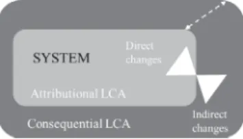
Fig. 1 – Boundaries of Attributional and Consequential LCA. Rectangles in light and dark grey represent the system boundaries respectively in Attributional and Consequential LCA. The boundaries of system expansion are represented by the white arrow. The Functional Unit (FU) is represented by white triangles. FU is defined according to ISO 14040 standards (Comité Technique, 2006a) as the quantified performance of a product system for use as a reference unit. In Attributional LCA, FU represents a portion of inventory and only direct changes, while either direct or indirect consequences due to FU are taken into account in Consequential LCA.

and land-use (Hauschild et al., 2013). A large amount of LCA works have been conducted concerning electricity production (Curran et al.,2001,2005;Davidsson et al.,2012;Gagnon et al.,

2002;Hawkes,2010;Mallia and Lewis, 2013;May and Brennan, 2003;Treyer and Bauer, 2013, 2014;Turconi et al.,2013).

Furthermore, LCA is in constant methodological develop-ment. Over the past two decades, Consequential LCA (CLCA) (Weidema,1993;Earles and Halog, 2011;Guiton and Benetto, 2013) has emerged as a modelling approach to assess conse-quences of changes (Ekvall, 2002). CLCA as a macro-systemic approach differs from classical Attributional LCA (ALCA) which is generally applied at a micro-system level (Guiton and Benetto, 2013). The main differences in both LCA ap-proaches refer to goal and scope as well as inventory steps.

Weidema et al.(1999) showed that Consequential modelling implies changes from Attributional in unitary processes in-teractions to expand the system, so that both direct and indi-rect impacts have to be considered, which is not the case in ALCA. CLCA has been discussed since the nineties (Weidema,

1993;Weidema et al.,1999) but its development is more re-cent. Indeed,Zamagni et al.(2012) emphasized the evolution of this method with an increasing number of publications de-voted to “Consequential” and “LCA” as keywords, highlight-ing the growhighlight-ing interest of LCA practitioners for assesshighlight-ing the consequences of change in addition to product Attributional assessments.

Inventory in CLCA yet requires specific inventory data, especially to assess indirect changes (Ekvall,2002;Weidema et al., 1999). The quality of inventory data is crucial for a reliable assessment: variability in Consequential Life Cycle Inventory (CLCI) may lead to uncertain LCIA results and may hamper the development of CLCA. Several methodologies using economic models to evaluate those data are available in the reported literature (Weidema et al., 1999). As CLCA includes all processes (direct and indirect) affected by change, some processes or energy fluxes remain in most studies (Guiton and Benetto, 2013; Weidema et al., 2009).

Fig. 1illustrates the main differences between Attributional and Consequential assessment mainly affecting system boundaries and direct/indirect changes.

Electricity, as a major energy provider for processes (Fernandez Astudillo et al.,2015), is intrinsically often taken into account in system expansion with indirectly affected processes. But, in some cases, the lack of data concerning electricity makes practitioners exclude electricity change

Table 1 – Selected countries for typology design. Each country is selected from its total production in 2012 superior to 10 TWh (The Shift Project, 2015).

Africa Asia Middle East Europe America Oceania

Algeria Azerbaijan Kyrgyzstan Bahrain Austria Iceland Argentina Australia Egypt Bangladesh Lao Iran Belarus Ireland Brazil New Zealand

Ghana India Malaysia Iraq Belgium Italy Canada

Morocco Indonesia Sri Lanka Israel Bulgaria Netherlands Chile Mozambique Pakistan Taiwan Oman Croatia Norway Colombia Nigeria Philippines Tajikistan Qatar Denmark Poland Cuba South Africa Singapore Thailand Saudi Arabia Estonia Portugal Ecuador Zambia Japan Uzbekistan Jordan Finland Romania Mexico Tunisia Kazakhstan Viet Nam Kuwait France Russia Paraguay

Hong Kong China Lebanon Georgia Serbia Peru Lybia Germany Slovakia Uruguay

Syria Greece Slovenia USA

United Arab Emirates Hungary Spain Venezuela Bosnia and

Herzegovina

Sweden Dominican Republic Switzerland

Czech Republic Turkey UK Ukraine

(Ekvall and Andrae, 2006), or take too general data in databases (Fernandez Astudillo et al.,2015). Only short-term country-level data have recently become available in the literature (Amor et al., 2014).

A consistent approach concerning electricity production for CLCA has not been established till now to our knowledge and the development of more generalized electricity production CLCI data represents a major challenge for CLCA application (Zamagni et al.,2012;Ekvall and Andrae, 2006). If short-term country-level data start to be available in literature, reliable data are still lacking in a long-term perspective.

A first step to address this issue is to better understand electricity production mix worldwide. The aim of this work is to set a typology of electricity production mixes, based on potential greenhouse gas (GHG) emissions for electricity production and mix composition. Even if only GHG emissions are considered, the conceptual framework of LCA is used for several reasons: (i) LCA is particularly interesting as a system-oriented environmental assessment method; (ii) the typology that will be proposed could be further used for Consequential LCA which is the core of the work and (iii) could be finally extended to other criteria. Specific attention will thus be given to the relation between GHG for electricity production and mix composition factors in order to determine a mix typology.

2.

Material and methods

The first step of the proposed methodology is to determine an appropriated time scale for the study. The year 2012 is used a starting reference date to observe the effects of energy transition, following the growing concerns about GHG emissions and global warming (OECD/IEA, 2014; den Elzen et al.,2014).

The typology has to be representative of most of mixes in the world. To avoid bias in the analysis, a well-established database and a set of representative countries must be taken into account. For this purpose, a same database for typology

design is used. A freely accessible online world database that is TSP Database fromThe Shift Project(2015) has thus been selected. TSP data portal is an information platform that provides a free access to a wide range of global energy and climate statistics and combines data from IEA (OECD/IEA,

2015) andThe World Bank(2015) in downloadable excel files. The typology will have to be also representative of global mix dynamics. For this purpose, only countries with significant annual electricity production capacity will be considered. A preliminary screening of the potential of the electricity production of a more exhaustive list of countries shows that several production levels (5, 10, 20 TWh) can be highlighted. In that context, a 10 TWh level can be viewed as an average value for representing the minimal production level of the countries that will contribute to the typology. This finally leads to a set of 91 countries from every continent to be considered in the analysis.

2.2. Data collection and calculation of GHG emissions

The typology is based on two kinds of data, first, mix composition, expressed in percentage of the total production in 2012, and secondly GHG emissions of an energy amount of 1 kWh.

2.2.1. Mix composition

Using TSP Database (The Shift Project,2015), the electricity generation data for the 91 countries satisfying a minimal production of 10 TWh used in this study are listed inTable 1.

The primary resources and their related power plants taken into account in the typology are biomass and waste, coal, gas, geothermal, hydroelectric, hydroelectric pumped storage, nuclear, oil, solar/tide/wave and wind.

2.2.2. GHG emissions

GHG emissions are defined here as the potential greenhouse gas (GHG) emissions per kWh calculated using LCA methods. Well-established and average values for GHG emissions are required for the typology design. As shown byHauschild et al.

(2013), the best way to evaluate climate change is to use the IPCC (The Intergovernmental Panel on Climate Change) baseline model of 100-year model and radiative forcing based

Table 2 – GHG emissions vs. type of primary resource, from SREEN report (Moonmaw et al., 2011). GHG emissions represent potential emissions in

gCO₂eq/kWh, from LCA results.

Type of primary resource GHG emissions in gCO₂eq/kWh

Biopower and waste 18

Coal 1001

Gas 469

Geothermal 45

Hydroelectric (pump storage included) 4

Nuclear 16

Oil 840

Solar/Tide/Wave 46

Wind 12

on global warming potential (GWP100), provided in the SREEN report, Appendix II, Table A.II.4 Strunz (2014) and Herbert et al.(2015). From the available data, the computation of the 50th _{percentile has been considered as a good compromise}

between all the technological specificities. The technologies represented in Table A.II.4 of the SREEN report (Moonmaw et al., 2011) are arranged in the same manner as in the definition of the mix composition adopted in this study.

For example, biomass and waste are merged in the proposed terminology and considered separately in the SREEN report. So, in order to use single LCA data for that case, we calculate the mean between non-aggregated of SREEN global warming potentials, that is, the mean between global warming potential of biomass and of that of waste thus obtaining an aggregated value.

The LCA results that will be used in our calculations are presented inTable 2:

Considering each country from i = 1 to 91 and using data from mix composition, the GHG emission for each primary resource m (for a total of 9), of each country is computed as follows:

GHG_i,m= (Qm/Q_Tot)×GHGm for m = 1 to 9 (1)

GHG_i,m: GHG emission of the primary resource for the country i in gCO₂eq/kWh

Qm: quantity of electricity produced by primary resource in TWh

Q_Tot: total production in TWh

GHG_m: GHG emission of the primary resource in gCO₂eq/kWh. The cumulative calculation for all primary resources then gives:

CF_i=X

m

(Qm/Q_Tot×GHGm) (2)

m: primary resource

CF_i: GHG emissions for country i in gCO₂eq/kWh.

This method is implemented for the 91 countries considered in the study.

2.3. Typology development

2.3.1. Ranking and boundary definition

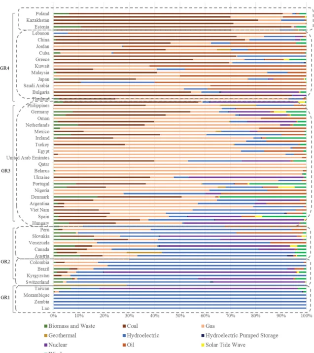
Fig. 3 presents the GHG emissions ranked from the less to the most emitting country and Fig. 4 displays the mix composition histogram per country.

First, the GHG emissions are analysed to identify the occurrence of a change in the curve (for example plateau or increase) that may constitute the boundary of a potential

Fig. 2 – Determination of theoretical mixes from typology boundaries—B_infand Bsupcorrespond respectively to the

lower and upper bounds, that have been identified by the 2-tuple (GHG emissions CF; mix composition MC). The different steps allow determining (CFs; MCs) corresponding

to the theoretical bound Bs.

group. Second, the mix composition histogram is analysed concurrently to establish if the observed change in GHG emissions is correlated with a mix change. In case of agreement, the boundaries of a group are identified as boundary candidates that will be further considered for typology development.

2.3.2. Building theoretical typology boundaries

The typology must represent every possible mix. As mentioned in Section 2.2.2, the first step of our work only gives discrete values corresponding to the GHG emissions of the studied countries. The objective is here to determine the theoretical mixes that can represent general compositions as shown inFig. 2, so that the evolution of GHG emissions can be viewed as a continuous function of the mix composition. Even if numerous combinations of mixes can correspond to identical values of GHG emissions, the theoretical mix has to correspond to the really observed ones that define potential boundaries.

For this purpose, the following methodology is proposed to determine theoretical mixes. For the sake of illustration, an arbitrary example supports the methodology: the numerical values do not represent the results that have been actually observed.

For each potential boundary defined in Section 2.2.2, the GHG emissions and mix composition can be obtained. For example, let us consider two consecutive values of potential boundaries for a same group, i.e., 450 gCO₂eq/kWh and 590 gCO₂eq/kWh respectively. The first emission value (respectively the second one) corresponds to a mix composed of 90% gas (which contributes to 422.1 gCO₂eq/kWh) and of a 10% contribution of diverse renewables (which contribute to 27.9 gCO₂eq/kWh). The mix corresponding to 590 gCO₂eq/kWh is also composed of 90% of gas (which contributes to 422.1 gCO₂eq/kWh as abovementioned) and of

Fig. 3 – GHG emissions for the selected countries, GHG emissions are ranked in increasing order, the changes in curves identified. Grey arrows correspond to intervals delimiting boundaries before their evaluation regarding mix composition and leading to six potential groups: black arrows correspond to the finally selected intervals for boundary determination. The term GR is the abbreviation of the final group.

10% of a really diverse mix of fossil and renewables (which contributes to 167.9 gCO₂eq/kWh).

Similarities and differences between both mix composi-tions can thus be observed and the level of gCO₂eq/kWh that each contributor (i.e. energy primary source) gives can thus be highlighted. It must be also emphasized that the determi-nation of a continuous function between two bounds is also motivated by the identification of a bound expressed as an integer rounded to hundred (here 500 gCO₂eq/kWh). In the example, both mixes have in common the gas contribution that will be kept for theoretical mix. The remaining energy sources then contribute to 77.9 gCO₂eq/kWh, which is con-sistent with the observed mixes, that are largely composed of renewables, so that low emissions are involved, yet with some percents of fossil fuels (for example to back up demand change). It can be thus deduced that the theoretical boundary of 500 gCO₂eq/kWh is reached with a mix composed of 90% of gas and 10% of a diverse mix, majorly composed of renew-ables, but also of some fossil fuels.

By definition, a lower bound of a group will be the upper bound of the previous one.

2.3.3. Typology group description

A qualitative analysis is performed for each country in order to identify the characteristics that can globally represent every mix belonging to a group. These general characteristics about mix composition must be applicable to every possible mix and will then define a typology group. A maximum number of three qualitative features is considered.

This qualitative assessment will be performed by his-togram analysis (see Section2.3.1) for each mix in order to detect which types of primary resources are significant. A pri-mary resource is viewed as significant in mix composition for the typology if it represents at least 25% of the total mix com-position. These observations will form the basis for the deter-mination of major global characteristics of a group.

In order to avoid an exhaustive classification, i.e., limiting the number of features to 3, the primary resources that have similar values for GHG emissions and so a similar influence on mix are merged. This is typically the case for nuclear energy and hydropower, corresponding respectively to 4 and 16 gCO₂eq/kWh.

2.3.4. Final typology

The typology involves two items for group definition as defined in Sections2.3.2and2.3.3:

- GHG emission range, defined by continuous quantitative data of GHG emission results delimited by group boundaries,

- Mix composition global characteristics, encompassing the identification of primary resources used to produce electricity and their quantitative contribution.

In order to represent all the cases taken into account in the typology, a spatial representation using a Geographic Information System (GIS) (Heywood et al., 1998) that is well adapted for a multifaceted description of complex systems and their dynamics is used. For this purpose, QGIS 2.6.1 (QGIS, 0000), a widely used open source software tool for GIS representation and modelling is selected.

For each country, two kinds of information are visualized, i.e., first total electricity production for 2012 (see Section2.2.1 The Shift Project,2015), and second, typology group.

The same tool will be further used to represent the temporal evolution of the mix dynamics that will also be studied in a perspective of energy transition.

3.

Results and discussion

3.1.1. Representation of GHG emissions and mixes

Fig. 3shows the GHG emissions of the different countries that exhibit a nonlinear behaviour.

Six ranges can be observed in the GHG emission curve corresponding to a change in the curve: [16–30], [30–100], [100–230], [230–317], [317–570] and [570–800] gCO₂eq/kWh, leading to six potential groups.

It can be seen from the coloured patterns in Fig. 4that the mix composition histograms exhibit 3 major composition types, i.e., hydroelectric, gas and coal. Three characteristics can thus be highlighted for group definition and description.

Fig. 4 – Mix composition for the selected countries, GHG emissions are ranked in increasing order. Each grey border corresponds to potential groups represented by grey arrows inFig. 3. Black brackets on left side represent the selected groups (black arrows inFig. 3). The term GR is the abbreviation of the final group.

3.1.2. Group boundaries and mix composition

Three of the observed changes in the GHG emission curve can be found consistent with the typology, i.e., the existence of a potential boundary matches with a significant change in mix composition. The first occurrence corresponds to a GHG emission of 16 gCO₂eq/kWh representing mixes that are largely composed of hydraulic and nuclear production (grey arrow in Fig. 3). A break into mix composition can be observed, affecting no major production, that is nuclear and/or hydropower, but the other modes that are composed largely of fossil fuels and renewables to a less extent. So the range [4–16] gCO₂eq/kWh can be kept as a group (Gr 1). Let us consider now the range [100–230] gCO₂eq/kWh, corresponding to the third grey arrow in Fig. 3. Even if a change in the curve can be observed at the upper bound, it does not correspond to a major change in mix

composition. Indeed, hydropower plays an important role in mix. This explains why the two domains [30–100] and [100–230] gCO₂eq/kWh can be merged together to form group Gr 2. Indeed, the mixes in that group have a major production mode composed mainly of nuclear and/or hydropower, and of other production modes composed of various primary resources, from renewables to fossils fuels. The range [317, 570] gCO₂eq/kWh, corresponding to the fourth grey arrow in Fig. 1, is well representative of mixes composed of gas as major production, and of various other production mixes, so that the range [317–570] can be considered as group Gr3. Finally, the break occurring at 800 gCO₂eq/kWh, corresponding to the last grey arrow inFig. 1, involves mixes with a majority of high emitting fossil fuel, i.e., coal and fuel so that it does seem necessary to distinguish between them.

Table 3 – World mix typology. Each group is characterized by boundaries defined by GHG emissions of kWh, major production, which represent predominant primary resources and other production mode that match total mix composition.

Group GHG Bounds (gCO₂eq/kWh) Main characteristics

Major production Other production

1 Very low 0–37 Hydraulic and/or nuclear Predominantly renewables 2 Low 37–300 Hydraulic and/or nuclear Diversification

3 Average 300–600 Gas Diversification

4 High >600 Coal, oil Predominantly fossils

The identification of potential boundaries deduced from a graphical analysis is then followed by the analysis of theoretical mixes, so that the typology initiated from discrete values of carbon emissions of a set of countries could be extended to continuous values. Concerning the first group [4–16] (gCO₂eq/kWh), the mixes are mainly composed of hydraulic and nuclear production, as observed in Fig. 4. The lower bound has been taken equal to zero, so that the potential of new technologies that will be less emitting than hydropower (which is at 4 gCO₂eq/kWh) can be further considered. Clearly, a mix exclusively composed of either nuclear or hydraulic can be viewed as difficult to manage in a majority of cases, due to short-term demand management, for countries that do not have a strong grid connection with their neighbours or back-up generating capacity provided by others. So, to be consistent with this assumption, a bound with a theoretical mix composed of 75% of hydraulic or nuclear and 25% of a low emitting mean mix (composed of gas and renewables) has been selected, leading to an upper bound set at 37 gCO₂eq/kWh. For the second group ranging from [30–230] gCO₂eq/kWh from the graphical interpretation, the upper bound of the range has to represent mixes with high diversity in electricity generation, either from fossil or renewable sources, as it can be seen in Fig. 3. However, the value of carbon emissions of 230 gCO₂eq/kWh seems to be low compared to the following break observed at 317 gCO₂eq/kWh. A compromise solution involving a theoretical mix distributed between gas (50%) and a low emitting average mix (50%), including renewables, gas and only coal or fuel, leads to a bound of 300 gCO₂eq/kWh. For the third group, the observed upper bound (570 gCO₂eq/kWh) is determined by a theoretical mix mostly composed of gas and an average mix based on a variety of production means, (i.e., renewables, fossil fuels, hydropower etc.). A rounded value of 600 gCO₂eq/kWh is finally adopted and is consistent with the graphical observation and the principle of “continuity “for the carbon emission evolution vs. mix composition. No upper bound has been fixed for Gr 4.

3.1.3. Final typology

From the results mentioned above, the final topology can be proposed as follows (Table 3).

As suggested in3.1.1, it can be first highlighted that the groups differ from each other by three major production types: hydraulic and/or nuclear, gas and coal that have been merged in the typology into fossil fuels (oil being scarcely represented).

At first look and without considering the typology, it can be said that only major production conditions group affiliation. So the other production modes, i.e., those representing less than half of total production are also key components in the affiliation to a group or another. For instance, the difference between Gr 1 and 2 is due to the diversity of those other

production modes. The same comment is valid for Gr 3 and 4, but in that case, the diversity benefit to GHG emissions that can be observed is lower.

Then two supergroups corresponding to groups, which have the same characteristics about their major productions, i.e. Gr1, 2 and Gr 3,4, respectively can be observable in the typology. This assumption could imply different efforts for instance to move from the emitting supergroup 3–4 to the supergroup 1–2 or to move through a supergroup in a dynamic vision of mixes involved in an energy transition.

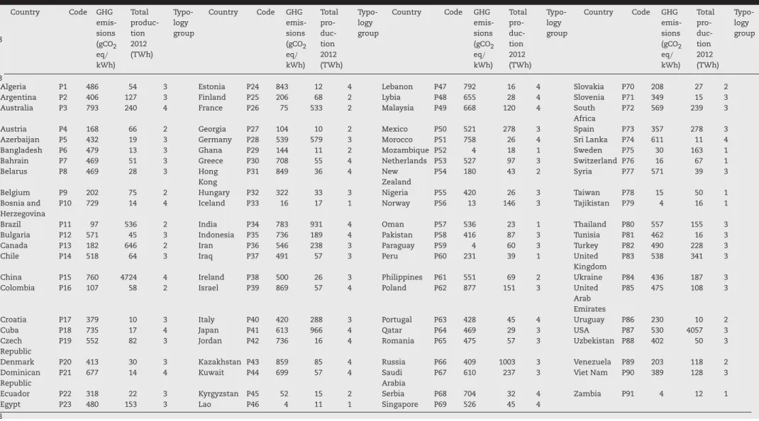
The country-level data are available in Appendix A,

Table A.

3.1.4. World representation of the typology

The typology can also be visualized through a map representation to give more information about countries and their groups, as shown in Fig. 5. First, it can be observed that the main producers are also those belonging to Gr 4 with the highest GHG emissions, i.e., China and India, United States, Russia and some European countries such as Spain, Germany or United Kingdom. An energy shifting towards a more virtuous group can be achieved through a drastic change in their electrical mix. The Japan case requires special attention as 2012 corresponds to one year after Fukushima events: Japan had to replace its nuclear production by other modes, such as coal and oil, which are highly emitting production means. But this change is temporary, since the reactivation of some nuclear power plants in 2016 (Nuclear Energy Institute, 0000). So Japan could be a good candidate to observe a quick evolution from a highest emitting group to lower ones.

Latin America is the lowest emitting continent, with five among seven countries being part of low emitting supergroups 1–2, with significant electricity production in Brazil.

Africa is mostly not represented in typology, due to too low electricity production under 10 TWh for 2012.

The European case can also give some guidelines to analyse the United States dynamics. As Europe, the United States is composed of states with strongly different mixes. Indeed, even if the energy transition in the United States has to be considered globally, the way that each of the 50 states can achieve such a transition by 2050 has also to be taken into account.

3.2. Understanding long-term dynamics of mixes

3.2.1. Uncertainty on group boundaries

The analysis on the determination of group boundaries is based on median results (Section3.1.2). The objective of this section is to show how uncertainty may affect results. For this purpose, a sensitivity analysis is carried out using the same methodology as the one presented in Section 2.3.2,

Fig. 5 – Typology and total production, per country. The circle size is proportional to total production in 2012 for countries, which produced more than 10 TWh as presented inTable 1.

Fig. 6 – GHG emissions for the selected countries, ranked in increasing order. The dotted lines correspond to the previous bounds for the intervals determined from the median value. The black arrows correspond to the finally selected intervals for boundary determination. The grey zones correspond to the intervals calculated using the 25thand 75thpercentiles for GHG emissions: transition zone 1 from Gr 1 to 2, [11; 71] covering 6 countries, transition zone 2 from Gr 2 to 3, [235; 311] covering 1 country and transition zone 3 from Gr 3 to 4 [536; 693] covering 15 countries.

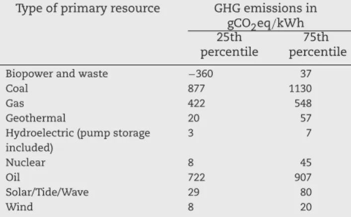
with the 25th and 75th percentiles as respective lower and upper bounds for GHG emission. As before, the data from IPCC (Moonmaw et al., 2011) are used (seeTable 4).

The obtained results are visualized inFig. 6and highlight the difference between the variation in major production and the one in other production mode. Transition zone 1 (corresponding to interval [11; 71]), with an amplitude of 60 gCO₂eq/kWh, (belonging to supergroup 1) exhibits the same major production but presents some variations in other production mode. The mix diversity leads in most cases to more emitting results. For example even if a variation of

1% or 2% in gas contribution seems insignificant, it has a significant influence on the total GHG emissions of the mix. The amplitude of 60 gCO₂eq/kWh may thus be viewed as the uncertainty embedded in the mass contribution of the mix, which may contribute significantly to total GHG emissions.

For transition zone 2 (corresponding to interval [235; 311]), major production changes from hydroelectric and/or nuclear to gas. So the results between those two groups are generally marked, and uncertainty appears to be low considering the relative values of GHG emissions. Moreover, it emphasizes the transition from supergroup 1–2 to supergroup 3–4.

Table 4 – Percentiles of GHG emissions vs. type of primary resources, from SREEN report (Moonmaw et al., 2011). GHG emissions represent the potential emissions in gCO₂eq/kWh, from LCA results.

Type of primary resource GHG emissions in gCO₂eq/kWh 25th

percentile

75th percentile

Biopower and waste −360 37

Coal 877 1130

Gas 422 548

Geothermal 20 57

Hydroelectric (pump storage included) 3 7 Nuclear 8 45 Oil 722 907 Solar/Tide/Wave 29 80 Wind 8 20

Transition zone 3 (corresponding to interval [536; 693]) has an amplitude of 157 gCO₂eq/kWh (corresponding to the interval [536; 693]). The observed uncertainty is significant and comes from the uncertainty in GHG emissions of the dominant production means in Gr 3 and 4. Indeed, when technologies such as gas, coal or fuel exhibit a high uncertainty in their GHG emissions, the uncertainty calculated for a global mix which is majorly composed of those kinds of technologies will be also high.

These transition zones could be useful to be observed for implementing energy policies and for leading to a more comprehensive set of recommendations for future research and policy. Indeed, they allow to identify a state where mixes of a group start to have characteristics from another one. Then, those transition zones could lead to a better understanding of the implications of transitions. This can already be observed in two examples, Denmark and France.

Denmark has recently achieved a major change in its mix composition by introducing renewables (Mathiesen et al., 2009), especially wind power, moving from Gr 4 to Gr 3 in the 2000s. This transition is a result of energy policies established since the seventies to move from a mix majorly based on coal or oil to a more virtuous one composed of renewables. The transition zones constitute good tool to identify how long the transition has taken to move permanently from Gr 4 to Gr 3. In the case of France, since the first oil crisis in 1973, the French government has decided to introduce nuclear power into the electricity mix to decrease the national energy dependency (Percebois, 2012). This leads to a change in the proposed typology from Gr 3 to Gr 2, and the analysis of mix composition in this transition zone could give us insight to better understand how this change has been conducted. Then, from historical mix dynamics, the typology can thus serve as a tool to identify how much time countries will take to achieve major changes and how such a transition can be characterized.

3.2.2. Influence of network

It must be emphasized that the interconnection of electricity networks between countries is not taken into account in the typology. However, the grid interconnection across countries can be viewed as a key feature in mix evolution. Indeed, some countries have a small production in their territory and benefit from their neighbours’ production. This situation can offer the opportunity to some countries to have a more

virtuous mix: this corresponds typically to some countries from Gr 1 or 2 with a lot of intermittent renewables, for which most of their demand is produced by their neighbours and transported through existing networks. This can be in some cases explained by a lack in resources (either natural or technological) so that a real dependency on network supply is observed.

The ratio of net imports (US Department of Energy,

2016) compared to total production (The Shift Project,2015) expressed in percentage is represented inFig. 7. A majority of countries use grid connection with imports and exports: a value of 10% either for exports or imports is considered to be significant.

The exchanges that have been considered are available in

Appendix A,Table B.

As it can be seen in Fig. 7, the most virtuous countries from Gr 1, are most of the time net exporters. So, clearly, the quality of their mix is due to their own electricity generation. Exporting such power can be beneficial to the grid-connected countries. Besides, major importers, i.e. countries importing more than 10% of their energy belong mostly to Gr 3 and 4. So, even if a switch from a group to a more eco-friendly one for these countries is not impossible, it can be viewed as difficult to steer their energetic policy onto a markedly different energy path. A closer look at Group 2 shows that importers and exporters, (respectively major and small ones) are equally involved. So the network dependency may not be significant for these countries.

Of course we are aware thatFig. 7only gives the general trend about network influence. A more thorough analysis could be yet carried out in order to include over time small power producers, for example African countries, which could be highly network-dependent. In addition, indicators and performance measures of the interdependence of a country from the grid must be properly defined and included in the typology. This highlights to consider the energy infrastructure with a systems approach.

3.2.3. Inertia in electricity power generation and resilience to energy change

As emphasized in Section 3.1.3, major power generation systems play a key role in the typology by defining the supergroup in which mixes are, i.e., less emitting with major production of hydraulic and/or nuclear and higher emitting with major production based on gas and fossil fuels.

If those elements are now considered in a dynamic perspective, three types of changes could affect the existing mixes. In an energy transition point of view, every country will try to move to a less emitting group. So a shifting towards a higher-emission group could be viewed as a temporary situation due to an increase in power demand that cannot be provided by low-carbon emitting technologies.

The first evolution type that can be considered involves changes within either “major” or “other production” groups, but these changes are not enough significant to create a definitive change of group. In these conditions, mixes evolve in the same group, or move to another one, but not permanently, thus corresponding to an incremental dynamics.

The second evolution type is relative to changes in “other production” modes so that Gr 4 (respectively 2) moves to Gr 3 (respectively to 1).

Finally, the evolution type that can be considered leads to drastic changes in major production, so that groups 4 or 3 can move to group 2 or 1, so that a breakthrough change occurs.

Fig. 7 – Comparison of imports and export by typology group. Countries considered are the ones selected for designing the typology presented inTable 1. 10% is the limit between a high/low exporter or importer.

Of course, such evolutions are subject to system inertia. For example, a predominantly fossil-oriented mix e.g. from Gr 4 will have to diversify gradually its “other production” mode to move to another group, and changes will require some years to finally reach Gr 3.

Furthermore, due to country specificities, inertia may be different for each group, depending on the strategy of each country concerning major electricity power generation. This aspect can be considered as a key feature for mix evolution. This criterion of inertia has to be further taken into account in the typology.

It is also important to consider flexibility and robustness. The guarantee of good resistance to shocks, sometimes referred to as resilience, is another parameter that must be considered in energy policies. It can lead to particular choices, not only in terms of diversification, or supply structures and energy system technologies, but also in terms of R&D, so that, a wide range of technologies and skills is available.

These elements are particularly important to be examined in a typology definition in order to determine the horizon time, which will be necessary for a country to shift to another group. This suggests that an indicator based on resilience of a country’s energy system can be useful to measure the effectiveness of adaptation policies addressing such issues as energy generation.

3.2.4. A step towards a better understanding of global energy transition

As demonstrated in a previous work (Herbert et al., 2015), only major evolutions could lead to a lasting mix change. This dynamics can be initiated by modifying one or a range of static drivers, such as existing power plants, resources, technological developments (such as energy storage, carbon capture and storage), energy policy and public opinion. Some of these drivers can be considered formally in a dynamic modelling of the energy system to determine energy policies. Other criteria such as public opinion are yet more subjective but their influence may be significant on the other factors. For example, public opinion will strongly influence energy policy and can make it change, as observed in Italy concerning nuclear power (OECD/IEA, 2009).

Moreover, all countries are unequal face to those elements: there are among them differences in the way the possible mixes are assessed and thus in how an ideal or more practically an optimum mix (if it does exist) can be reached in terms of kWh GHG emissions (either both direct and indirect) and mix composition. Preferences vary widely

from country to country, for example between levels of development (Northern and Southern countries) or domestic resources. As aforementioned, an indicator measuring the capacity to implement energy adaptation projects and how successful the proposed implementation measures will be in increasing energy system resilience will be particularly useful (Michaelowa et al., 2010).

This approach could also help to better understand energy transition communication with a clearer vision of the potential evolution of energy systems.

The use of generalized data in the proposed typology could thus strongly benefit in decision-making processes, especially for the development of new climate policy and related research. Indeed, for illustration purposes, the electricity production mix could be envisioned not as a compilation of production means, which would evolve with the addition or withdrawal of production means as “pieces”, but rather as a single malleable entity, which would evolve by stretching. The typology could help identify which kind of mix is observed and which transition is possible from a group to another one and when the “malleable entity” will move to another type of mix with different main characteristics. As highlighted in Section3.2.1, the transition zones could give an easy way to identify potential energy transition dynamics.

Finally whereas the typology is helpful, the importance of country-level results should not be downplayed. LCA results that are commonly used are likely to vary significantly by country depending on factors such as the vintage of the generation fleet as well as that of the supply chain infrastructure. Yet, the typology gives results and key tendencies at a high level of granularity and so does not take into account those specific country-level data. The typology can be viewed as a tool to identify the process dynamics and key evolutions tendencies, about an energy transition, with no specific insight of the country considered. The analysis of the mix dynamic evolution of some selected countries could thus give more insight to establish the limit between the use of typology and the one of specific country-level data at a lower level of granularity.

3.3. Typology use in Consequential inventories

Literature review highlights that CLCA studies have been carried out with data on case by case basis (Earles and Halog, 2011). Such an approach is both time and expertise consuming. Moreover, available techniques from Weidema et al. (1999,2009)and Ecoinvent (Treyer and Bauer, 2013, 2014)

do not make consensus for LCA practitioners (Fernandez Astudillo et al., 2015), especially concerning uncertainty management. In most studies, CLCA involves general equilibrium and partial equilibrium models to estimate economy-wide indirect emissions, which are subject to many types of uncertainty. In that context, all consequences that follow are not generally well taken into account. The literature review has shown that Consequential LCA suffers from a lack of knowledge of potential consequences from a policy examined, data gaps and large uncertainties, as well as from a lack of models that can capture the dynamic changes in land use patterns in different countries under specific economic drivers. Other indicators have been identified in the reported literature as relevant for electricity production impacts (Hauschild et al., 2013; PEFCR, 2015), such as resource depletion, water footprint, acidification and eutrophication. The Intergovernmental Panel on Climate Change (IPCC) Fourth Assessment Report (AR5) (Edenhofer et al., 2014) states, with very high confidence, that the observed changes in global climate are very likely due to the increase in anthropogenic greenhouse gas (GHG) concentrations. This is also emphasized in a recent SCORE LCA study (Alexandre et al., 2014) showing that according to practitioners responding to climate change involves to mitigate the emissions of greenhouse gases in the atmosphere.

The proposed typology can be considered as a first step to bridge this gap by considering typical groups of electricity power generation, in a worldwide and environmental vision. It must yet be strengthened by the development of indicators reflecting resilience to energy change and grid interconnection.

The development of the typology is interesting to represent the behaviour of some countries that share the same characteristics in a group. Then, data calculated from a mean mix representing each group could give easy to set data. With the selection of some countries in each group as a test bench, we could evaluate if global dynamics and data could be set by analysing the evolution of mixes through time in the typology, and otherwise what could be carried out to estimate them. This work will explore prospective data from public prospective studies available for each country selected. Conceptually, prospective studies estimate different future evolutions of current mixes (Pottier, 2014). Furthermore, in Consequential LCA thinking, mixes strongly evolve through time leading to allocation problems (Guiton and Benetto, 2013). Then, those results could constitute first methodological steps to establish Consequential LCI datasets.

4.

Conclusions

Generalizing world electricity mixes production is a first step to evaluate the feasibility evaluation of Consequential spe-cific inventory data. That is why a typology for mix as-sessment based on two criteria evaluated for 91 selected countries, i.e., mix composition (both qualitatively and quan-titatively) and GHG emissions. Four groups have thus been established according to GHG emission range Gr1, very low (0–37 gCO₂eq/kWh); Gr2 low (37–300 gCO₂eq/kWh); Gr3 mean (300–600 gCO₂eq/kWh) and Gr4 high (>600 gCO₂eq/kWh) emitting countries. The GHG emissions have been associated with main characteristics of energy portfolio based on major

and “other” modes for electricity power generation. Following this analysis, two supergroups {Gr 1; Gr 2} and {Gr 3; Gr 4} have been established based on major production mode. A map representation has shown the distribution of a set of coun-tries (91) among the identified groups and subgroups and the possible path these countries are likely to carry out for achiev-ing their energy transition. Moreover, this typology allows qualifying the change degree needed to achieve energy tran-sition. Indeed, a transition is represented by a group change, involving either major or small productions, and the zone of uncertainty between groups could help identifying transition dynamics. The proposed typology can thus also be seen as an energy transition evaluation tool.

However, in order to use this typology in a Consequential LCI perspective, some criteria have to be developed in more depth. Firstly, national and cross-borders electrical grid networks are fundamental in electricity mix consumption, and this issue has to be considered in the further development of the typology by a so-called network indicator. Secondly, all the countries are not equal in terms of mix evolution inertia, so that an indicator based on energy sector resilience can be added. Lastly, linked to changing effort and inertia, tools to evaluate how mix can reach a so-called optimal group are required. These energy mix assessment criteria will be useful to evaluate Consequential inventory mix in order to reach a given target.

The proposed typology gives thus a macro-level vision of electricity production mixes that is more general than the level vision. Of course, to set reliable country-level dataset, additional factors have been completed to ensure reliable country-level datasets such as efficiency of country-level generation fleets, transmission and distribution losses, capacity factors, and higher-resolution generation detail (e.g. are natural gas plants peak or base-load for instance). The integration of grid modelling could constitute a further extension of this work. To support temporal dataset development, short-term (hourly) data from grid should be needed. The conciliation of short-term and long-term data will be probably required since in a long-term perspective. The influence that grid development and network may have on mix dynamics has to be investigated.

The next step towards the evaluation of typology to design generalized Consequential inventory data concerning electricity production is to study the dynamic evolution of some countries selected from each group of the proposed typology using historical data.

Acknowledgements

Funding: This work was supported by EDF R&D (SIRET 552 08131778287).

The authors would like to thank Miguel Lopez Botet Zulueta (EDF R&D OSIRIS), Sandrine Leclercq, Vincent Morisset, Yann Le Tinier (EDF R&D EPI), and Pr. Stephan Astier (INP Toulouse) for their fruitful review and suggestions about this work.

Appendix

Table A – Selected countries for typology design with associated code in manuscript, GHG emissions (calculated with Section 2.2.2 methodology), total production for 2012 and group in presented typology. Countries are alphabetically ranked.

48 Country Code GHG emis-sions (gCO₂ eq/ kWh) Total produc-tion 2012 (TWh) Typo-logy group Country Code GHG emis-sions (gCO₂ eq/ kWh) Total pro- duc-tion 2012 (TWh) Typo-logy group Country Code GHG emis-sions (gCO₂ eq/ kWh) Total pro- duc-tion 2012 (TWh) Typo-logy group Country Code GHG emis-sions (gCO₂ eq/ kWh) Total pro- duc-tion 2012 (TWh) Typo-logy group 48

Algeria P1 486 54 3 Estonia P24 843 12 4 Lebanon P47 792 16 4 Slovakia P70 208 27 2

Argentina P2 406 127 3 Finland P25 206 68 2 Lybia P48 655 28 4 Slovenia P71 349 15 3

Australia P3 793 240 4 France P26 75 533 2 Malaysia P49 668 120 4 South

Africa

P72 569 239 3

Austria P4 168 66 2 Georgia P27 104 10 2 Mexico P50 521 278 3 Spain P73 357 278 3

Azerbaijan P5 432 19 3 Germany P28 539 579 3 Morocco P51 758 26 4 Sri Lanka P74 611 11 4

Bangladesh P6 479 13 3 Ghana P29 144 11 2 Mozambique P52 4 18 1 Sweden P75 30 163 1

Bahrain P7 469 51 3 Greece P30 708 55 4 Netherlands P53 527 97 3 Switzerland P76 16 67 1

Belarus P8 469 28 3 Hong

Kong

P31 849 36 4 New

Zealand

P54 180 43 2 Syria P77 571 39 3

Belgium P9 202 75 2 Hungary P32 322 33 3 Nigeria P55 420 26 3 Taiwan P78 15 50 1

Bosnia and Herzegovina

P10 729 14 4 Iceland P33 16 17 1 Norway P56 13 146 3 Tajikistan P79 4 16 1

Brazil P11 97 536 2 India P34 783 931 4 Oman P57 536 23 1 Thailand P80 557 155 3

Bulgaria P12 571 45 3 Indonesia P35 736 189 4 Pakistan P58 416 87 3 Tunisia P81 462 16 3

Canada P13 182 646 2 Iran P36 546 238 3 Paraguay P59 4 60 3 Turkey P82 490 228 3

Chile P14 518 64 3 Iraq P37 491 57 3 Peru P60 231 39 1 United

Kingdom

P83 538 341 3

China P15 760 4724 4 Ireland P38 500 26 3 Philippines P61 551 69 2 Ukraine P84 436 187 3

Colombia P16 107 58 2 Israel P39 869 57 4 Poland P62 877 151 3 United

Arab Emirates

P85 475 108 3

Croatia P17 379 10 3 Italy P40 420 288 3 Portugal P63 428 45 4 Uruguay P86 230 10 2

Cuba P18 735 17 4 Japan P41 613 966 4 Qatar P64 469 29 3 USA P87 530 4057 3

Czech Republic

P19 552 82 3 Jordan P42 736 16 4 Romania P65 475 57 3 Uzbekistan P88 402 50 3

Denmark P20 413 30 3 Kazakhstan P43 859 85 4 Russia P66 409 1003 3 Venezuela P89 203 118 2

Dominican Republic

P21 677 14 4 Kuwait P44 699 57 4 Saudi

Arabia

P67 610 237 3 Viet Nam P90 389 128 3

Ecuador P22 318 22 3 Kyrgyzstan P45 52 15 2 Serbia P68 704 32 4 Zambia P91 4 12 1

Egypt P23 480 153 3 Lao P46 4 11 1 Singapore P69 526 45 4

Table B – Net imports in TWh for selected countries of typology from 2009 to 2012 from EIA (eia.gov) with associated code in manuscript. Negative results correspond to exports and positive results to imports.

Country Code2009 2010 2011 2012 Country Code2009 2010 2011 2012 Country Code2009 2010 2011 2012 Country Code2009 2010 2011 2012

Algeria P1 0.0 −0.1 −0.1 0.0 Estonia P24 0.1 −3.3 −3.6 −2.2 Lebanon P47 1.2 1.2 0.8 0.3 Slovakia P70 1.3 1.0 0.7 0.4 Argentina P2 6.2 8.6 9.7 7.6 Finland P25 12.1 10.5 13.9 17.4 Lybia P48 0.0 −0.1 −0.1 0.0 Slovenia P71 −3.1 −2.1 −1.3 −0.9 Australia P3 0.0 0.0 0.0 0.0 France P26 −25.9 −30.7 −56.4 −44.5 Malaysia P49 −0.1 −0.2 0.4 0.1 South

Africa

P72 −1.8 −2.5 −3.1 −5.0 Austria P4 0.8 2.3 8.2 2.8 Georgia P27 −0.5 −1.3 −0.5 0.1 Mexico P50 −0.7 −0.7 −0.6 −0.7 Spain P73 −8.1 −8.3 −6.1 −11.2 Azerbaijan P5 −0.3 −0.4 −0.7 −0.5 Germany P28 −12.3 −15.0 −3.8 −20.5 Morocco P51 4.6 3.9 4.6 4.8 Sri Lanka P74 0.0 0.0 0.0 0.0 Bangladesh P6 0.2 0.2 0.1 −0.2 Ghana P29 −0.6 −0.9 −0.6 −0.5 Mozambique P52 −5.1 −3.5 −3.4 −1.5 Sweden P75 4.7 2.1 −7.2 −19.6 Bahrain P7 0.0 0.0 0.0 0.0 Greece P30 4.4 5.7 3.2 1.8 Netherlands P53 4.9 2.8 9.1 17.1 Switzerland P76 −2.2 0.5 2.6 −2.2 Belarus P8 4.5 2.7 5.6 7.6 Hong

Kong

P31 7.9 8.4 8.4 10.0 New Zealand P54 0.0 0.0 0.0 0.0 Syria P77 −0.1 −0.4 0.3 1.2 Belgium P9 −1.8 0.6 2.5 9.9 Hungary P32 5.5 5.2 6.6 8.0 Nigeria P55 0.0 0.0 0.0 0.0 Taiwan P78 0.0 0.0 0.0 0.0 Bosnia

and Herzegovina

P10 −3.0 −3.8 −1.5 0.0 Iceland P33 0.0 0.0 0.0 0.0 Norway P56 −9.0 7.5 −3.1 −17.8 Tajikistan P79 0.1 0.1 0.0 −0.7

Brazil P11 40.0 34.6 35.9 40.3 India P34 5.3 5.5 5.1 4.8 Oman P57 0.0 0.0 0.0 0.0 Thailand P80 1.1 6.0 9.7 9.0 Bulgaria P12 −5.1 −8.4 −10.7 −8.3 Indonesia P35 0.0 0.0 0.0 0.0 Pakistan P58 0.2 0.3 0.3 0.4 Tunisia P81 0.0 0.0 0.0 0.0 Canada P13 −33.4 −25.3 −36.7 −46.6 Iran P36 −4.1 −3.7 −5.0 −7.1 Paraguay P59 −45.0 −43.4 −46.1 −47.7 Turkey P82 −0.7 −0.8 0.9 4.3 Chile P14 1.3 1.0 0.7 0.0 Iraq P37 5.6 6.2 7.3 8.2 Peru P60 −0.1 −0.1 0.0 0.0 United

Kingdom

P83 2.9 2.7 6.2 12.0 China P15 −11.4 −13.5 −12.8 −10.8 Ireland P38 0.8 0.5 0.5 0.4 Philippines P61 0.0 0.0 0.0 0.0 Ukraine P84 −5.4 −4.1 −6.3 −5.9 Colombia P16 −1.1 −0.8 −1.5 −0.7 Israel P39 −3.8 −4.0 −4.2 −4.4 Poland P62 −2.2 −1.4 −5.2 −2.8 United

Arab Emirates

P85 0.0 0.0 0.0 0.0

Croatia P17 5.1 4.1 7.4 11.5 Italy P40 45.0 44.2 45.7 43.1 Portugal P63 4.8 2.6 2.8 7.9 Uruguay P86 1.2 −0.3 0.5 0.5 Cuba P18 0.0 0.0 0.0 0.0 Japan P41 0.0 0.0 0.0 0.0 Qatar P64 0.0 0.0 0.0 0.0 USA P87 34.1 26.0 37.3 47.3 Czech

Republic

P19 −13.6 −14.9 −17.0 −17.1 Jordan P42 0.2 0.6 1.7 0.7 Romania P65 −2.3 −2.3 −1.9 −2.8 Uzbekistan P88 −0.1 −0.1 −0.1 −0.1 Denmark P20 0.3 −1.1 1.3 5.2 Kazakhstan P43 −0.7 1.2 0.8 1.3 Russia P66 −14.9 −17.4 −22.6 −16.5 Venezuela P89 −0.4 −0.4 −0.5 −0.2 Dominican

Republic

P21 0.0 0.0 0.0 0.0 Kuwait P44 0.0 0.0 0.0 0.0 Saudi Arabia P67 0.0 0.0 0.0 0.0 Viet Nam P90 3.7 4.6 1.8 2.2 Ecuador P22 1.1 0.9 1.3 0.2 Kyrgyzstan P45 −1.2 −1.7 −2.7 −1.7 Serbia P68 −1.4 −0.3 −0.3 0.4 Zambia P91 −0.6 −0.6 −0.6 −0.6 Egypt P23 −0.9 −1.4 −1.6 −1.4 Lao P46 −1.1 −5.1 −9.0 −8.4 Singapore P69 0.0 0.0 0.0 0.0

References

Alazard-Toux, N., Criqui, P., Devezeaux de Lavergne, J.-G., 2013. Scénarios de l’ANCRE pour la transition énergétique Rapport 2013’, Agence Nationale de la Coordination de la Recherche et de l’Energie, France.

Alexandre, C., Gérard, A., Goedkoop, M., Ponsioen, T., 2014. Environmental impact indicators in LCA: state of the art, feedback and recommendations’, SCORE LCA, Villeurbanne, France, Guide for LCA practitioners - final Study N˚ 2013-04, Nov.

Amor, M.B., Gaudreault, C., Pineau, P.-O., Samson, R., 2014. Implications of integrating electricity supply dynamics into life cycle assessment: A case study of renewable distributed generation. Renew. Energy 69, 410–419.

Comité Technique ISO/TC 207 and CMC, 2006a. ‘NF EN ISO 14040 (2006-10-01) - Management environnemental, Analyse du cycle de vie, Principes et cadre’, AFNOR, France, Norme, Oct. Comité technique ISO/TC 207, 2006b. ‘ISO 14044:2006 - Manage-ment environneManage-mental, Analyse du cycle de vie, Exigences et lignes directrices’, ISO, Norme, Jul.

Curran, M.A., Mann, M., Norris, G., 2001. Report on the Inter-national Workshop on Electricity Data for Life Cycle Inven-tories’, NREL, EPA, Breidenbach Research Center, Cincinnati, Ohio, EPA/600/R-02/041, Oct.

Curran, M.A., Mann, M., Norris, G., 2005. The international workshop on electricity data for life cycle inventories. J. Cleaner Prod. 13 (8), 853–862.

Davidsson, S., Höök, M., Wall, G., 2012. A review of life cycle assessments on wind energy systems. Int. J. Life Cycle Assess. 17 (6), 729–742.

den Elzen, M., Fekete, H., Admiraal, A., Forsell, N., Höhne, N., Korosuo, A., Roelfsema, M., van Soest, H., Wouters, K., Day, T., 2014. Enhancing ambition in the major emitting countries’, PBL/NewClimate Institute/IIASA/Ecofys, Dec.

Earles, J.M., Halog, A., 2011. Consequential life cycle assessment: a review. Int. J. Life Cycle Assess. 16 (5), 445–453.

Edenhofer, O., Pichs-Madruga, R., Sokona, Y., Minx, J.C., Farahani, E., Kadner, S., Seyboth, K., Adler, A., Baum, I., Brunner, S., Eickemeier, P., Kriemann, B., Savolainen, J., Schlömer, S., von Stechow, C., Zwickel, T., 2014. IPCC (Intergovernmental Panel on Climate Change): Climate change 2014: Mitigation of climate change. Working Group III contribution to the IPCC Fifth Assessment Report. Cambridge University Press, Cambridge, United Kingdom and New York, NY, USA.

Ekvall, T., 2002. Limitations of Consequential LCA’, LCA/LCM 2002 E-Conference, 20-May.

Ekvall, T., Andrae, A., 2006. Attributional and consequential environmental assessment of the shift to lead-free solders (10 pp). Int. J. Life Cycle Assess. 11 (5), 344–353.

Fernandez Astudillo, M., Treyer, K., Bauer, C., Ben Amor, M., 2015. Exploring challenges and opportunities of life cycle management in the electricity sector. In: Life Cycle Management. Springer, pp. 295–306.

Finnveden, G., Moberg, Å, 2005. Environmental systems analysis tools – an overview. J. Cleaner Prod. 13 (12), 1165–1173. Gagnon, L., Bélanger, C., Uchiyama, Y., 2002. Life-cycle

assess-ment of electricity generation options: The status of research in year 2001. Energy Policy 30 (14), 1267–1278.

Geels, F.W., Schot, J., 2007. Typology of sociotechnical transition pathways. Res. Policy 36 (3), 399–417.

Guiton, M., Benetto, E., 2013. Analyse du Cycle de Vie Conséquentielle?: Identification des conditions de mise en oeuvre et des bonnes pratiques’, CRP Henri Tudor, Luxembourg, SCORELCA Etude A2012_01.

Hauschild, M.Z., Goedkoop, M., Guinée, J., Heijungs, R., Huijbregts, M., Jolliet, O., Margni, M., Schryver, A.D., Humbert, S., Laurent, A., Sala, S., Pant, R., 2013. Identifying best existing practice for characterization modeling in life cycle impact assessment. Int. J. Life Cycle Assess. 18 (3), 683–697.

Hawkes, A.D., 2010. Estimating marginal CO2 emissions rates for national electricity systems. Energy Policy 38 (10), 5977–5987.

Herbert, A.-S., Azzaro-Pantel, C., Le Boulch, D., 2015. Key drivers of a common dynamic vision of electricity production mix using IPCC 2007 GWP 100a indicator’, presented at the Life Cycle Management 2015, Bordeaux.

Heywood, I., Cornelius, S., Carver, S., 1998. An introduction to Geographical Information Systems. Longman, Harlow. Hopwood, D., 2015. The world waits for COP to deliver. Renew.

Energy Focus 16 (5–6), 91.

Mallia, E., Lewis, G., 2013. Life cycle greenhouse gas emissions of electricity generation in the province of Ontario, Canada. Int. J. Life Cycle Assess. 18 (2), 377–391.

Mathiesen, B.V., Münster, M., Fruergaard, T., 2009. Uncertainties related to the identification of the marginal energy technology in consequential life cycle assessments. J. Cleaner Prod. 17 (15), 1331–1338.

May, J.R., Brennan, D.J., 2003. Application of data quality assessment methods to an LCA of electricity generation. Int. J. Life Cycle Assess. 8 (4), 215–225.

Michaelowa, A., Connor, Hè., Williamson, L.E., 2010. Use of indicators to improve communication on energy systems vulnerability, Resilience and adaptation to climate change. In: Troccoli, Netherlands, A. (Ed.), Management of Weather and Climate Risk in the Energy Industry. Springer, Dordrecht, pp. 69–87.

Moonmaw, W., Burgherr, P., Heath, G., Lenzen, M., Nyboer, J., Verbruggen, A., 2011. IPCC Special Report on Renewable Energy Sources and Climate Change Mitigation. In: Edenhofer, O., Pichs-Madruga, R., Sokona, Y., Seyboth, K., Matschoss, P., Kadner, S., Zwickel, T., Eickemeier, P., Hansen, G., Schlömer, S., von Stechow, C. (Eds.), Cambridge, United Kingdom, New York, NY, USA.

Nuclear Energy Institute. ‘Japan Nuclear Update - Nuclear En-ergy Institute’. [Online]. Available: http://www.nei.org/News-Media/News/Japan-Nuclear-Update[Accessed: 25.05.16]. OECD/IEA, 2009. ‘Energy Policies of IEA Countries - Italy 2009

Review’, IEA, Paris, France.

OECD/IEA , 2014. Energy, Climate Change and Environment: 2014 Insights - Executive Summary. International Energy Agency, Paris, France, Available:

https://www.iea.org/Textbase/npsum/EECC2014sum.pdf. OECD/IEA, 2015. ‘International Energy Agency website’,

In-ternational Energy Agency website, [Online]. Available:

http://www.iea.org/.

PEFCR Pilot PV electricity generation, 2015. ‘Production of photovoltaic modules used in photovoltaic power systems for electricity generation (NACE/CPA class 27.90 “Manufacturing of other electrical equipment”)’, European Union, Product Environmental Footprint Category Rules, Sep.

Percebois, J., 2012. Rapport Energie 2050’, Centre d’analyse stratégique, Gouvernement français, France.

Pottier, A., 2014. L’économie dans l’impasse climatique (Thèse d’Economie), CIRED, Paris.

QGIS Community. ‘QGIS Software - version 2.6.1 Brighton.

Strunz, S., 2014. The German energy transition as a regime shift. Ecol. Econ. 100, 150–158.

The Shift Project, 2015. ‘Historical Electricity Generation Statis-tics’, The Shift Project Data Portal, [Online]. Available:

http://www.tsp-data-portal.org/.

The World Bank, 2015. ‘The World Bank (IBRD -IDA), Data’, The World Bank, Data, [Online]. Available:

http://data.worldbank.org/.

Treyer, K., Bauer, C., 2013. Life cycle inventories of electricity generation and power supply in version 3 of the ecoinvent database—part I: electricity generation. Int. J. Life Cycle Assess. 1–19.

Treyer, K., Bauer, C., 2014. Life cycle inventories of electricity generation and power supply in version 3 of the ecoinvent database—part II: electricity markets. Int. J. Life Cycle Assess. 1–14.

Turconi, R., Boldrin, A., Astrup, T., 2013. Life cycle assessment (LCA) of electricity generation technologies: Overview, compa-rability and limitations. Renewable Sustainable Energy Rev. 28, 555–565.

United Nations, 2016. Framework convention on climate change. In: Report of the Conference of the Parties on its twenty-first session, held in Paris from 30 November to 11 December 2015. Addendum. Part two: Action taken by the Conference of the Parties at its twenty-first session., United Nations, Paris, France, FCCC/CP/2015/10/Add.1, Jan.

US Department of Energy, 2016. ‘International Energy Statistics -EIA’, EIA.gov, [Online]. Available: http://www.eia.gov/cfapps/ ipdbproject/IEDIndex3.cfm?tid=2&pid=2&aid=23 [Accessed: 04.01.16].

Verbong, G., Geels, F., 2007. The ongoing energy transition: Lessons from a socio-technical, multi-level analysis of the Dutch electricity system (1960–2004). Energy Policy 35 (2), 1025–1037.

Verbong, G.P.J., Geels, F.W., 2010. Exploring sustainability transi-tions in the electricity sector with socio-technical pathways. Technol. Forecast. Soc. Change 77 (8), 1214–1221.

Weidema, B.P., 1993. Market aspects in product life cycle inventory methodology. J. Cleaner Prod. 1 (3–4), 161–166.

Weidema, B.P., Ekvall, T., Heijungs, R., 2009. Guidelines for application of deepened and broadened LCA, Deliverable D18 of work package 5 of the CALCAS project’, CALCAS, Project no.37075, Jun.

Weidema, B.P., Frees, N., Nielsen, A.-M., 1999. Marginal production technologies for life cycle inventories. Int. J. Life Cycle Assess. 4 (1), 48–56.

Zamagni, A., Guinée, J., Heijungs, R., Masoni, P., Raggi, A., 2012. Lights and shadows in consequential LCA. Int. J. Life Cycle Assess. 17 (7), 904–918.