HAL Id: tel-01525432
https://pastel.archives-ouvertes.fr/tel-01525432
Submitted on 20 May 2017
HAL is a multi-disciplinary open access
archive for the deposit and dissemination of
sci-entific research documents, whether they are
pub-lished or not. The documents may come from
teaching and research institutions in France or
abroad, or from public or private research centers.
L’archive ouverte pluridisciplinaire HAL, est
destinée au dépôt et à la diffusion de documents
scientifiques de niveau recherche, publiés ou non,
émanant des établissements d’enseignement et de
recherche français ou étrangers, des laboratoires
publics ou privés.
systems
Loïc Henriet
To cite this version:
Loïc Henriet. Non-equilibrium dynamics of many body quantum systems. Quantum Physics
[quant-ph]. Université Paris-Saclay, 2016. English. �NNT : 2016SACLX036�. �tel-01525432�
Je remercie tout d’abord les rapporteurs, professeurs J. Keeling et W. Zwerger, d’avoir accept´e de lire et de porter un oeil critique sur mon manuscrit. Je tiens aussi `a re-mercier les autres membres du jury d’avoir accept´e d’assister `a ma soutenance.
La plus grande reconnaissance va `a Karyn Le Hur, qui a constamment suivi avec soin mon parcours de th`ese. Ses id´ees toujours excellentes ont su guider mon effort, et sont `a l’origine de beaucoup de ce qui est pr´esent´e dans ce manuscrit. Merci pour la confiance qu’elle m’a accord´ee.
Merci `a tous les membres du Centre de Physique Th´eorique pour leur accueil et leur gentillesse. Je remercie particuli`erement mon parrain Christoph Kopper pour sa gentillesse et sa disponibilit´e, ainsi que Bernard Pire qui nous avait soutenu Lucien et moi lors de notre tentative de mise en place d’un s´eminaire pour les doctorants et post-doctorants du laboratoire. Un grand merci `a Fadila, Florence, Jeannine, Malika ainsi qu’`a Danh, David, et Jean-Luc pour leur aide. J’aimerais aussi souligner ma reconnaissance envers l’Ecole Polytechnique, et j’en profite aussi pour remercier tous les professeurs qui ont influenc´e mon parcours et m’ont pouss´e `a poursuivre en th`ese. Merci `a Peter Orth et Zoran Ristivojevic pour leur aide pr´ecieuse au d´ebut de ma th`ese et leurs conseils pour aborder un probl`eme scientifique. Leur contribu-tion au d´eveloppement de l’approche stochastique pr´esent´ee dans ce manuscrit est `a souligner particuli`erement. Il est aussi important de mentionner que cette technique a ´et´e ´elabor´ee suivant les id´ees d’Adilet Imambekov, que je n’ai pas eu le plaisir de connaˆıtre. J’ai aussi eu l’opportunit´e de pouvoir travailler en collaboration avec An-drew Jordan et je le remercie pour sa gentillesse et ses id´ees ´eclairantes. J’ai aussi beaucoup appr´eci´e travailler avec Guillaume Roux et Marco Schir´o, et les remercie pour cette chance. Je salue aussi Guang-wei Deng et le remercie pour le dialogue que nous avons pu lier entre th´oriciens et exp´erimentateurs lors de notre collaboration. Ces ann´ees de th`ese m’ont aussi permis d’int´eragir avec de nombreux groupes de recherche et je tiens `a remercier les universit´es de Bˆale, Cologne, Heifei, Orsay, Princeton, Stony Brook, Ulm, ainsi que l’Ecole Normale Sup´erieure, le CEA-Saclay et l’ICFO –et plus particuli`erement Christoph Bruder, Darrick Chang, Sebastian Diehl, Jean-No¨el Fuchs, Guo-Ping Guo, Susana Huelga, Christophe Mora, Olivier Parcollet, Fr´ed´eric Pi´echon, Dominik Schneble, Pascal Simon, et Hakan T¨ureci. Je remercie aussi les organisateurs de l’´ecole Physique m´esoscopique au Qu´ebec et du GdR CNRS `a Aussois, l’Institut
Canadien de Recheche Avanc´ee, et les organisateurs de Qlight 2016 en Crˆete. Sur un plan plus personnel, je remercie Camille, Michele, et Marco pour les dis-cussions que j’ai pu avoir avec eux. Merci `a tous les anciens et actuels membres du groupe: Peter, Zoran, Alex, Tianhan, Lo¨ıc, Kirill, et Antonio avec qui j’ai eu le plaisir de collaborer pendant son stage de master.
` A C´ecile,
Introduction 11
1 Spin-Boson models 13
I Rabi model and applications . . . 13
I.1 Rabi Hamiltonian in cavity quantum electrodynamics . . . 14
I.1.a Charges in a box . . . 14
I.1.b Cavity Quantum electrodynamics setup . . . 14
I.1.c Weak-coupling regime and Jaynes-Cummings physics 16 I.2 Rabi Hamiltonian in circuit quantum electrodynamics . . . 17
I.2.a Artificial atom: the Cooper pair box . . . 18
I.2.b Cavity: The superconducting resonator . . . 19
I.2.c Strong coupling regime beyond the RWA . . . 21
I.3 Many-body physics in large circuits . . . 23
I.3.a Arrays of cavities . . . 24
I.3.b Driven-dissipative problem . . . 24
I.3.c Mean field quantum phase transition in the adiabatic regime . . . 26
II Ohmic spinboson model . . . 28
II.1 Modelling of dissipation . . . 29
II.2 Quantum phase transition and relation with Kondo model . . . 29
II.2.a Polaron ansatz and quantum phase transition . . . 29
II.2.b Relation with Kondo model . . . 31
II.3 Circuit quantum electrodynamics: semi-infinite transmission line 33 II.4 Spinboson model in a cold-atomic setup . . . 34
II.5 Non-equilibrium dynamics and NIBA equation . . . 37
2 SSE equation and applications 39 I SSE Equation in the case of one spin . . . 40
I.1 Feynman-Vernon influence functional . . . 42
I.2 “Blips” and “Sojourns” . . . 44
I.3 Stochastic unravelling . . . 47
II Properties of the SSE equation . . . 48
II.1 Non-unitarity and trace preservation . . . 49
II.2 Dynamical sign problem . . . 49
II.4 NIBA from the SSE . . . 50
II.5 Relation to other methods . . . 51
III Application : dynamics in the quantum Rabi model . . . 51
III.1 Strong coupling regime . . . 52
III.1.a From the Jaynes-Cummings regime to the adiabatic regime . . . 52
III.2 Drive and photon losses . . . 52
III.2.a Polariton ⇡-pulse . . . 53
IV Application: dynamics in the ohmic spinboson model . . . 55
IV.1 Free dynamics and comparison with Bethe Ansatz results . . . 56
IV.2 Coherent-incoherent crossover around ↵ = 1/2 . . . 56
IV.3 Landau-Zener transitions . . . 58
IV.4 Mean field Landau Zener transitions in a dissipative spin array 58 IV.4.a Mean-field approximation in the SSE framework . . . 58
IV.4.b LZ transitions : Array . . . 61
3 Dynamics of two coupled spins in an ohmic environment 65 I Extension of the SSE framework to two spins . . . 65
II Nonequilibrium dynamics and quantum phase transition in the dimer model . . . 70
III Synchronization . . . 74
III.1 First mechanism . . . 75
III.2 Second mechanism . . . 77
4 Dissipative topological transition 81 I Topology of a spin 1/2 . . . 81
I.1 Chern number and Berry curvature . . . 82
I.2 Relation with topological properties of condensed matter systems 83 I.3 Coupling to an environment . . . 84
II Shifted oscillators approach to the transition . . . 84
III Experimental protocol . . . 86
IV Dissipative Spin dynamics and topology . . . 89
IV.1 Results for spin dynamics . . . 89
IV.2 Radiative cascade of photons and effective magnetic field . . . 91
V Toulouse point and critical behaviour . . . 92
VI Entanglement entropy and effective thermodynamics . . . 94
5 Hybrid electron-photon systems 97 I Nanoengine from quantum vacuum fluctuations . . . 98
I.1 Analysis . . . 99
I.2 Rectified current . . . 101
I.2.a Coupling to an ohmic environment . . . 101
I.2.b Coupling to a resonator . . . 104
I.3 Heat engine characteristics . . . 106
I.4 Conclusion and discussion about higher order terms . . . 108
II.1 SU(4) Kondo physics in a DQD device . . . 110
II.2 Light-matter coupling and Input-Output theory . . . 113
II.3 Experimental results at the charge degeneracy point A: Phase and Amplitude of Reflected Microwave Signal . . . 115
II.4 Interpretation of the experimentals measurements . . . 116
II.5 DC electron transport . . . 119
II.6 Evolution of the microwave response with temperature . . . 121
Conclusion and perspectives 123 Appendices A Derivation of the Feynman Vernon influence functional 127 I Path integral representation of the propagators P and Q . . . 128
II Stationary trajectories with Lagrange equations . . . 130
B Alternate derivation of Feynman-Vernon influence functional 133 C Blips and Sojourns decomposition 135 I Diagonal elements of the spin density matrix . . . 135
I.1 Contributions Jk,k,f,f . . . 135
I.2 Contributions Jk,k,f,f . . . 136
II Off-diagonal elements of the spin density matrix . . . 136
D Sampling of stochastic variables and convergence 139 I Fourier series decomposition . . . 139
II Definition of the stochastic fields in relation with autoregressive processes141 III Cutoffs and control parameters in the SSE framework . . . 141
E Additional developments on Blips and Sojourns re-writing 143 I Expressions of Mp1 and M p 2 . . . 143
II Scaling regime . . . 144
F Non-adiabatic response and topology 147 I Chern number and evolution of hσzi with ✓ . . . 147
II Proof of Eq. (4.18) using time-dependent perturbation theory . . . 147
Modern experimental platforms now allow to control and monitor interacting quan-tum systems in a precise manner. Motivated by quanquan-tum information purposes, these platforms are also of great interest to explore many-body quantum physics. The un-precedented control over the system’s parameters permits indeed to devise and tune desired Hamiltonians. This ability to emulate complex many-body Hamiltonian mo-tivates the development of precise theoretical predictions to better understand the physical phenomena underlying the system’s dynamics. Most experimental setups also involve periodic pumping of energy into the system, as well as dissipative effects, fostering the development of specific theoretical tools to tackle the dynamics in out-of-equilibrium conditions.
In Chapter I we introduce the class of Spin-Boson models and focus in particular on the Rabi model, the ohmic spinboson model, and their lattice versions. The Rabi model considers a two-level system coupled to a quantized harmonic oscillator and de-scribes the simplest interaction between matter and light. Its lattice version describing a set of interacting light-matter systems opens the door to many-body physics with light. The ohmic spinboson model was first introduced to describe dissipative effects on a two-level system. In this description dissipation is modelled by a bath of quantized harmonic oscillators, and many-body effects of the bath notably induce a dissipa-tive quantum phase transition at large spin-bath coupling (see “Many-Body Quantum Electrodynamics Networks: Non-Equilibrium Condensed Matter Physics with Light”). In Chapter II, we derive a Stochastic Schr¨odinger Equation (SSE) describing the time evolution of the spin-reduced density matrix for Spin-boson problems. We test this framework and recover known results for the dynamics of the Rabi model (see “Quantum dynamics of the driven and dissipative Rabi model”) and the ohmic spinbo-son model. We also compare the SSE approach to other known methods and present the limitations related to the SSE.
In Chapter III, we extend the applicability of the SSE to the case of two spins coupled to a common ohmic bosonic environment. We investigate the dissipative quantum phase transition induced by the bath, and study the quenched dynamics in both phases. We also focus on bath-induced synchronization effects between two spins with different frequencies (see “Quantum sweeps, synchronization, and Kibble-Zurek physics in dissipative quantum spin systems”).
In Chapter IV, we study the influence of an ohmic environment on the topological properties of a two-level system measured with a dynamical protocol. We show in par-ticular that the bath induces a dissipative topological transition at strong coupling, and we investigate the properties of this transition.
In Chapter V, we focus on hybrid devices coupling quantum dots and lead elec-tronic degrees of freedom to light. We first introduce and study theoretically a nano heat-engine setup consisting of a quantum dot coupled to fermionic (electronic) leads and different Left/Right bosonic environments (see “Electrical Current from Quantum Vacuum Fluctuations in Nano-Engines”). We show how zero-point quantum fluctu-ations stemming from bosonic environments permit the rectification of the current. Then we present and interpert the results of a recent experiment studying a double quantum dot setup coupled to a resonator. We establish a link between the light measurements and the formation of a SU(4) Kondo bound state at low temperatures (see “A Quantum Electrodynamics Kondo Circuit: Probing Orbital and Spin Entan-glement”).
Publication list:
• “Quantum dynamics of the driven and dissipative Rabi model”, L. Henriet, Z. Ristivojevic, P.P. Orth, K. Le Hur, Physical Review A 90 (2), 023820 (2014). • “Electrical current from quantum vacuum fluctuations in nanoengines”, L.
Hen-riet, A. N. Jordan, K. Le Hur, Physical Review B 92 (12), 125306 (2015). • “Quantum sweeps, synchronization, and Kibble-Zurek physics in dissipative
quantum spin systems”, L. Henriet, K. L. Hur, Physical Review B 93 (6), 064411 (2016).
• “Many-Body Quantum Electrodynamics Networks: Non-Equilibrium Condensed Matter Physics with Light”, K. Le Hur, L. Henriet, A. Petrescu, K. Plekhanov, G. Roux, M. Schir´o, Comptes Rendus Physique, 17 (8), 808-835 (2016). • “A Quantum Electrodynamics Kondo Circuit: Probing Orbital and Spin
Entan-glement”, G.-W. Deng, L. Henriet, D. Wei, S.-X. Li, H.-O. Li, G. Cao, M. Xiao, G.-C. Guo, M. Schir´o, K. Le Hur, G.-P. Guo, arXiv preprint arXiv:1509.06141 (2015).
CHAPTER
1
Spin-Boson models
In this chapter, we will intoduce the Rabi model and the ohmic Spinboson model as paradigmatic models to describe respectively light-matter interaction and decoher-ence. We will put a particular emphasis on the investigation of many-body physics phenomena related to these models. In the Rabi case, this notably includes the pos-sible realization of arrays of interacting light-matter elements, giving access to exotic phases where light behaves as a quantum fluid. In the ohmic spinboson case, many-body effects play naturally an important role and trigger a dissipative quantum phase transition at large coupling. Realizing dissipative arrays may allow to facilitate the investigation of this transition.
I
Rabi model and applications
The Rabi model had been originally introduced to describe the effect of a magnetic field on an atom possessing a nuclear spin [1, 2]. Nowadays, this model is applied to a variety of quantum systems in relation with strong light-matter interaction. It follows indeed naturally from the general description of a set of spinless point charges interacting with the quantized electromagnetic field. The Rabi model turns out then to be a paradigmatic model to describe cavity quantum electrodynamics experiments (cavity QED), in which an atom is placed inside a microwave or optical cavity. The introduction of cavity QED experiments and the derivation of the Rabi model in this context will be exposed in section I.1, following the general description provided in Refs. [3, 4].
In Sec. I.2, we focus on the description of so-called circuit quantum electrodynam-ics experiments (circuit QED), describing the interaction of an artificial atom made of superconducting materials with microwave photons. These systems permits to repro-duce the physics of the Rabi model on chip, with a very large light-matter coupling. Recent experimental progress in this field allows now to envision the creation of larger circuits composed of a large number of coupled light-matter elements, which are of particular interest to investigate many-body phenomena with light.
I.1
Rabi Hamiltonian in cavity quantum electrodynamics
I.1.a Charges in a boxWe consider a set of charges placed inside a three dimensional box of typical length L. The Hamiltonian describing these charges in interaction with the electromagnetic field reads in the Coulomb gauge [3] H = Hkin+ Hr+ Vcoul, with
Hkin= X ↵ [p↵− q↵A(r↵)]2 2m↵ (1.1) Hr= X k X n=1,2 ~!ka† k,nak,n. (1.2)
In Eq. (1.2), r↵ and p↵ are the position and momentum operators of the particle ↵
with charge q↵ and mass m↵. The vector potential A(r↵) is described by a set of
bosonic operators a†k,n and ak,n corresponding respectively to the creation and the
annihilation of a photon in the mode k with energy ~!kand polarization n 2 (1, 2).
A(r↵) = X k X n=1,2 r ~ 2✏0!kL3 ⇣ ak,neik.rα+ a†k,ne−ik.rα ⌘ ek,n, (1.3)
The frequencies !k,n are quantized in relation with the boundary conditions imposed
by the box, and the vectors ek,n correspond to the two possible polarizations for
the transverse vector potential. The kinetic term Hkin in Eq. (1.2) will describe
the interaction between the charges and the electromagnetic field through the vector potential. We remark from Eq. (1.3) that the vector potential grows as the size of the box we consider decreases. In the case of a small box the vector potential exists only as a superposition of a discrete set of modes. This interesting case led to the the design of cavity quantum electrodynamics experiments, where an atom placed inside a cavity interacts resonantly with the confined electromagnetic field.
I.1.b Cavity Quantum electrodynamics setup
In a typical cavity QED setup, the atom is chosen such that the transition energy ∆ between a reference state |gi and an excited state |ei is close to the energy ~!0of one
of the first modes of the confined light, in the microwave [5] or optical regime [6]. The joint evolution of the light-matter system inside the cavity will result from this resonant interaction, and the effect of higher harmonics will be neglected. The wavelength corresponding to the resonant mode under consideration is much greater than the atomic length-scale, so that one can safely replace the kinetic term Hkin in Eq. (1.2)
by Hkin= X ↵ [p↵− q↵A(0)]2 2m↵ , (1.4)
where we define r = 0 as the position of the atomic center of mass. This simplification is known as the long-wavelength approximation. Expanding Eq. (1.4) then leads to a
sum of three terms, Hkin = X ↵ p2↵ 2m↵− X ↵ q↵p↵ 2m↵ ! .A(0) +X ↵ [q↵A(0)]2 2m↵ . (1.5)
In most cavity-QED experiments, the last term on the right hand side of Eq. (1.5) can be neglected due to the smallness of the electromagnetic field [4]. The atom-field coupling is captured by the second term of Eq. (1.5) which can be understood better in terms of the dipole of the atom. Following Ref. [7], we write
p↵
m =
i
~[Hat, r↵] , (1.6)
where Hatwould be the Hamiltonian describing the atom without its interaction with
the electromagnetic field. Introducing the dipole operator
d=X
↵
q↵r↵, (1.7)
one can then write Hkin = X ↵ p2 ↵ 2m↵− i 2~[Hat, d] .A(0) + X ↵ [q↵A(0)]2 2m↵ . (1.8)
As stated previously, the atomic degree of freedom can be effectively described by a two-level system composed of the states |gi and |ei. The dipole operator is off-diagonal in this basis, as the atom is neutral. We call d = he|d|gi the dipole matrix element between the two atomic states and we reach the Hamiltonian
H = ✓ ∆ 2 0 0 −∆2 ◆ − iX n ∆ 2 1 p 2✏0~!0L3 ✓ 0 dn −d⇤ n 0 ◆ ) an+ a†n * +X n ~!0a†nan. (1.9) Considering only one light polarization and after a rotation in the atomic subspace, we reach the Rabi Hamiltonian,
HRabi= ∆ 2σ z+g 2σ x(a + a†) + ~! 0 ✓ a†a +1 2 ◆ (1.10) where the light-matter coupling strength g reads
g = p d∆
2✏0~!0L3
. (1.11)
In Eq. (1.10), σxand σz belong to the set of Pauli matrices,
σx= ✓ 0 1 1 0 ◆ σy= ✓ 0 −i i 0 ◆ σz= ✓ 1 0 0 −1 ◆ . (1.12)
I.1.c Weak-coupling regime and Jaynes-Cummings physics
The typical value of the light matter coupling in 3D optical [6] or microwave [5] cavity QED setups is of the order of g/(~!0) ⇠ 10−7. In this range of parameters and for
low detuning |∆ − ~!0|/(~!0) ⌧ 1, Eq. (1.10) can be simplified further with the
application of the rotating wave approximation (RWA). This approximation consists in neglecting the counter-rotating terms, (σ+a†+h.c.) where σ±= (σx±iσy)/2, which
do not conserve the number of excitations. This ensures a continuous U (1) symmetry and an associated conserved quantity, the polariton number N = a†a + σ+σ− (which counts the total number of excitations, as the sum of light and matter excitations). The resulting Hamiltonian is the Jaynes-Cummings Hamiltonian HJC [8],
HJC = ∆ 2σ z+g 2 ) σ+a + σ−a†*+ ~!0 ✓ a†a +1 2 ◆ . (1.13)
The Jaynes-Cummings Hamiltonian is easily diagonalized in the so-called dressed basis [8]. The ground state of the system consists of the two-level system in its lower state and vacuum for the photons, while the excited eigenstates |n±i are pairs of com-bined light-matter excitations (polaritons) characterized by their polariton number. One has N |n±i = n|n±i. These eigenstates form the well-known structure of the
anharmonic JC ladder (Fig. 1.1). More precisely, the light-matter eigenstates satisfy (with n > 0):
|gi = | #z, 0i (1.14)
|n+i = ↵n| "z, n − 1i + βn| #z, ni (1.15)
|n−i = −βn| "z, n − 1i + ↵n| #z, ni, (1.16)
where | #zi and | "zi are the two eigenstates of σz with eigenvalues −1 and +1. The
corresponding energies are:
E|gi=δ 2 (1.17) E|n+i= n~!0+1 2 p δ2+ ng2 (1.18) E|n−i= n~!0−1 2 p δ2+ ng2. (1.19) We have ↵n = p [A(n) − δ] /2A(n), βn = p
[A(n) + δ] /2A(n), A(n) = png2+ δ2
and δ = ~!0 − ∆. Let us consider the case of an atom initially excited in an
empty cavity. Such a state is characterized by a wavefunction | i, which verifies | (t0)i = | "z, 0i = ↵1|1+i − β1|1−i, where t0 is the initial time. There is initially
one excitation in the system, which will be conserved during the dynamics. As the initial state is a superposition of the first two polaritons, we will observe an oscillation phenomenon in terms of the atomic and photonic observables hσzi and ha†ai. There
is a periodic exchange of energy between the atom and the field, a phenomenon called Rabi oscillations.
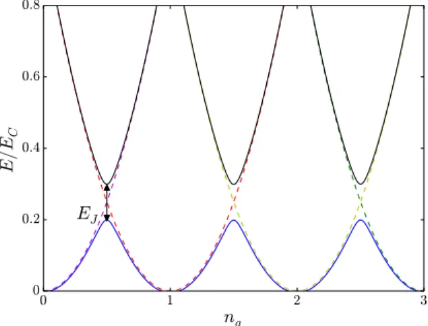
The Josephson tunneling mixes these two states and opens up a gap in the spectrum (see Fig. 1.3). All other charge states have a much higher energy and will be ne-glected in the following. Near these degeneracy points, the Cooper pair box can be described as an effective two level system. Let us consider for clarity that the
dimen-Figure 1.3: Eel(n, ng)/EC as a function of ng for n = 0 (dashed magenta), n = 1
(dashed red), n = 2 (dashed yellow) and n = 3 (dashed green). The blue and black lines show the eigenvalues of the total Hamiltonian HCP B(in units of EC) as a function
of ng. Here EJ= EC/10.
sionless gate voltage ng is close to 1/2, and we restrict the dynamics of the system
to the two states with either 0 or 1 excess Cooper pairs. In this basis, one can write HCP B = EJσ
x
2 − EC(1 − 2ng) σz
2 up to a constant term, where σ
x = |0ih1| + |1ih0|
and σz= |0ih0| − |1ih1|.
The effective field along the z-direction can be controlled dynamically by the gate voltage Vg. A magnetic control of the field along the x-direction is also possible if one
replaces the Josephson junction by a pair of junctions in parallel, each with energy EJ/2 (see [11]). In this case the transverse field becomes EJcos(⇡φ/φ0), where φ is
the magnetic flux in the loop formed by the two junctions and φ0= h/2e is the flux
quantum.
I.2.b Cavity: The superconducting resonator
The circuit-equivalent of the cavity consists in a section of a superconducting trans-mission line represented in Fig. 1.4. In the setup of Ref. [11], the artificial atom is directly placed at the center of the transmission line. The gate voltage acquires then a quantum part v, stemming from the fluctuations of the electromagnetic field inside the transmission line. The electromagnetic Hamiltonian Hel in Eq. (1.21) is replaced
leads to [11], HT L= 1 X p=1 h !2p ⇣ ~a†2pa2p+ 1/2⌘+ ~!2p−1⇣a† 2p−1a2p−1+ 1/2 ⌘i , (1.25) where !j = j⇡/(L p
lc). Even modes have voltage anti-nodes at x = 0, while odd modes have voltage nodes at x = 0, so that only the even modes participate to the voltage v coupled to the Cooper pair box at x = 0. If the energy of the mode p = 2 is close to EJ, one can neglect the modes of higher energy (note that the last term
on the right hand side of Eq. 1.23 renormalizes !2). After a ⇡/2 rotation in the spin
space, we recover the Rabi Hamiltonian HRabi from Eq. (1.10) for ng= 1/2, with the
identification: !0= !2 (1.26) ∆ = EJ (1.27) g = e Cg CJ+ Cg r ~!2 cL. (1.28)
These 1D circuit-QED systems allow to reach larger values of light matter cou-pling g/(~!) compared to their 3D cavity analogues [11] and constitutes one the most promising architecture for quantum computation.
I.2.c Strong coupling regime beyond the RWA
Light-matter coupling in these circuit QED experiments can reach g/(~!0) ' 10−1
[15]. In this regime, the rotating wave approximation breaks down and one must take into account the presence of the counter-rotating terms (σ+a†+ σ−a). The effect of
such terms can be understood in perturbation theory, and they give rise to a shift of the resonance frequency between the atom and photon, leading to an additional negative detuning in the energies plap (1.18) and (1.19)
δ ! δ − g2/ [2(~!0+ ∆)] , (1.29)
when ∆ < (~!0) (the levels repel each other). This so-called Bloch-Siegert shift [16]
has been observed in Ref. [15].
Another solvable limit, relevant to the strong coupling analysis of the Rabi model, is the so-called adiabatic regime [17, 18] or ”quasi-degenerate limit” [19–21]. This regime corresponds to a highly detuned system ∆/(~!0) ⌧ 1 with arbitrary large
light-matter coupling. One can visualize such a limit as a set of two displaced oscil-lator wells (characterized by the value of σx), whose degeneracy is lifted by the field
along the z-direction (see Fig. 1.5). At ∆ = 0, one can diagonalize separately the bosonic Hamiltonian, for the two values of σx, by looking for eigenstates |φ
eigenenergies E±: h ~!0a†a ±g 2(a + a †)i|φ ±i = E±|φ±i. ) ✓ a†±2!g 0 ◆ ✓ a ±2!g 0 ◆/ |φ±i = " E± ~!0 + ✓ g 2!0 ◆2# |φ±i. (1.30)
The operator on the left-hand side of Equation (1.30) can be re-expressed as D(⌥g/2!0)a†aD†(⌥g/2!0), where D(⌫) = exp[⌫(a† − a)] is a displacement
opera-tor [22]. This permits to find that eigenstates |φ±i correspond to displaced number
states |φ±,Ni = e⌥ g 2ω0(a†−a)|Ni ⌘ |N±i, (1.31) E±,N = ~!0 " N −✓ g2! 0 ◆2# . (1.32)
In Eq. (1.31), |Ni is a standard number state. The case N = 0 corresponds to well-known coherent states.
The lowest order adiabatic approximation consists in considering that the term ∆/2σzonly couples states in opposite wells with the same number of excitations. The
Hamiltonian can then be diagonalized as the number of displaced photons is a con-served quantity. A system initially prepared in a displaced state of one well would undergo coherent and complete oscillations between this state and its symmetric coun-terpart in the other well. The frequency of oscillations only depends on the overlap between these two states, and one can show that, starting from the N -th displaced state of one well, this frequency is Ω = ∆e−g2/2(~!
0)2L
N[g/(~!0)], where LN is the
N -th Laguerre Polynomial [18].
In these first two sections, we have explored two solvable limits of the Rabi model: • The Jaynes-Cummings regime corresponds to the limit g/(~!0) ⌧ 1 where the
RWA holds. The corresponding Hamiltonian (1.13) can be diagonalized in terms of mixed light-matter excitations named polaritons.
• The adiabatic regime corresponds to the limit ∆/(~!0) ⌧ 1. In this regime, the
Hamiltonian can be diagonalized in terms of superpositions of displaced number states.
Between these two clear limits one can use standard numerical methods, which allow to explore the time-evolution of dynamical quantities. Recently, analytical so-lutions of the quantum Rabi model have been explored in Refs. [23–26], based on the underlying discrete Z2 (parity) symmetry. Some dynamical properties of the model
have notably been addressed [27] thanks to this exact solvability. The link between the exact solvability and integrability of the Rabi model with related models such as the Dicke [28] model have also been studied [29]. Dicke model, which is the N spins version of the Rabi model, is notably known to exhibit a superradiant quantum
Figure 1.5: Two displaced wells characterized by the value of σx. This correspond to
the limiting case ∆ = 0. At first order in ∆/(~!0), one can consider that the term
in σz mixes only states corresponding to the same number of excitations of each well.
The energy splitting resulting from this term will be proportional to ∆ and to the overlap hN−|N+i = e−g
2
/2(~!0)2L
N[g/(~!0)].
phase transition in the limit N ! 1 [30]. By contrast to the Dicke model, the iso-lated quantum Rabi model does not exhibit a superradiant quantum phase transition when increasing the value of g/(~!0). This is illustrated on the left side of Fig. 1.1
where we see that the ground state and the first excited state do not cross when one increases the coupling g/(~!0), somehow illustrating the stability of an atom
inter-acting with a quantum field1. This must be contrasted by what would be predicted
by the Jaynes-Cummings model, for which crossings occur when g/(~!0) increases,
leading to unphysical polariton-like ground state.
I.3
Many-body physics in large circuits
In the past few years experimental progress was accomplished towards the realization of large arrays of circuit QED elements, where two neighbouring cavities i and j can be coupled using a capacitive or Josephson of the form J(ai+ a†i)(aj+ a†j). Assuming
that the coupling J between cavities is much smaller than the internal frequencies of the cavities, the coupling turns into an effective hopping term from one cavity to the neighboring ones. These architectures provide a robust architecture for solid-state quantum computation because of the unprecedented control over the system parameters and the low loss level. From a different viewpoint, they open a new way to explore many-body quantum systems in a precise and controllable manner.
1It is however important to note that the Rabi ground state contains a non-trivial photonic
I.3.a Arrays of cavities
From this perspective, one model that has been investigated a lot theoretically in the literature is the Jaynes-Cummings lattice model, which takes the form [31–33]:
Harray= X i HiJC− J X hi;ji ⇣ a†iaj+ a†jai ⌘ − µef f X i ⇣ a†iai+ σ+i σ−i ⌘ , (1.33) where Hi
JC describes the Jaynes-Cummings Hamiltonian in each cavity, introduced in
Eq. (1.13), and the summation is over nearest neighbors. This model has attracted some attention, for example, in the light of realizing analogues of Mott insulators with polaritons [34–37]. More precisely, one observes two competing effects in these arrays. For large values of J, formally the system would tend to form a wave delocal-ized over the full lattice, by analogy to a polariton superfluid [38], whereas for very small values of J, the photon blockade in each cavity will play some role. Theoretical works [34–37, 39], have focused on solving the phase diagram at equilibrium in the presence of a tunable chemical potential µef f.
For µef f = 0, the ground state at small J would correspond to the vacuum in
each cavity. By changing µef f and keeping J small, one could eventually turn the
vacuum in each cavity into a polariton state. Simple energetic arguments predict that this change would occur when E|1−i− µef f = E|gi. This result can be made more
formal by using a mean-field theory and a strong-coupling expansion [34–37]. In the atomic limit where J is small, one then predicts the analogue of Mott-insulating in-compressible phases, as observed in ultra-cold atoms [40], where it costs a finite energy to change the polariton number [32, 34, 41] (see Fig. 1.6). By increasing the hopping J, one can build an equivalent of the 4 theory, where ⇠ haii, in order to describe
the second-order quantum phase transition between the Mott region of polaritons and the superfluid limit [35].
I.3.b Driven-dissipative problem
Despite its great theoretical interest, this model is not readily implementable because no tunable chemical potential exists for photons. Similar to ultra-cold atoms [42, 43], it seems important to be able to engineer an effective chemical potential to develop further quantum simulation proposals and observe these Mott phase analogues. In Ref. [44], Hafezi and co-workers proposed to simulate an effective chemical potential for photons from a parametric coupling with a bath of the form λ cos(!pt)HSB where
HSB=Pj(aj+ a†j)Bj where Bj is a bath operator. Considerable attention has been
turned at a general level towards describing both driven and dissipative cavity arrays in order to realize novel steady states.
In realistic experimental conditions, photon leakage out of the system must indeed be taken into account. Each cavity is exposed to the vaccuum noise of the surrounding environment, and energy can leak out from the system. This effect can be addressed in a microscopic manner by considering a coupling of the inner photonic modes to
an infinite number of external bosonic modes, so that one must add to the system Hamiltonian the term (within a rotating-wave approximation) [45]:
X q ~!ql†qlq− iX q h fqa†ilq+ fq⇤ail†q i , (1.34) where l†
q (lq) is the creation (annihilation) operator of an external boson of frequency
!q. The use of the Heisenberg equations of motion in the Markov approximation, which
assumes that the coupling strength f =p|fq| and the density of state ⇢ =Pqδ(!−!q)
are constant, allows to write the effect of the environment as a imaginary component Γ = 2⇡f2⇢ for the photon frequency [45, 46].
In these conditions the system will eventually reach the ground state after a typical time of the order 1/Γ. To compensate this relaxation mechanism and access non-trivial states of matter, energy is often pumped into the system through the intermediary of an external time-dependent coherent drive on the cavity i [47, 48], of the form Vi(t)(ai+ a†i). One important point would then be to understand how the interplay
of drive and dissipation could play the role, or replace, the chemical potential µef f in
Eq. (1.33).
Let us study the effect of this driving term on the non-dissipative Jaynes-Cummings model (1.35).
HdJC = HJC+V0
2 (ae
i!dt+ a†e−i!dt). (1.35)
We can get rid of the time-dependent part of the Hamiltonian through a unitary transformation | ˜ i = U(t)| i with U(t) = exp⇥i!d(a†a + σ+σ−)t
⇤
. The evolution of | ˜ i is governed by the time-independent Hamiltonian ˜HRW A
sys : ˜ HsysRW A= ˜ ∆ 2σ z+ ˜! 0a†a + g 2(σ+a + σ−a †) +V0 2 (a + a †), (1.36)
where ˜∆ = ∆ − !d and ˜!0= !0− !d. ˜H is the sum of a JC Hamiltonian with
renor-malized energies ˜∆ and ˜!0, and a time independent driving term. It is convenient to
ex-press the last term of Eq. (1.36) in the dressed basis B = {|gi, |1, −i, |1, +i, |2, −i, |2+i, ...} of the coupled system [49]
a + a† = β1|1, +ihg| + ↵1|1, −ihg| + 1 X n=1 ⇥p n + 1βnβn+1+pn↵n↵n+1⇤|n + 1, +ihn, +| +⇥pnβnβn+1+ p n + 1↵n↵n+1 ⇤ |n + 1, −ihn, −| +⇥pn + 1↵n+1βn−pn↵nβn+1 ⇤ |n + 1, −ihn, +| +⇥pn + 1βn+1↵n−pn↵n+1βn ⇤ |n + 1, +ihn, −| +h.c.. (1.37)
Driving the cavity induces transition between the dressed states, and changes the num-ber N of excitations by ±1. As can be seen in Fig. (1.1), the Jaynes Cummings ladder is composed of two subladders of ‘minus’ and ‘plus’ polaritons. Eq. (1.37) illustrates the fact that the coupling between states of the same sub-ladder is stronger than the coupling between states which belong to different sub-ladders.
The interplay of drive, dissipation, and lattice effects make difficult the realiza-tion of an effective chemical potential µef f, motivating the development of numerical
schemes allowing to tackle the real-time dynamics of such driven dissipative models. One may mention the development of a nonequilibrium extension of stochastic mean-field theory in Ref. [50], applicable to problems of coupled cavities with rather general forms of driving and dissipation.
I.3.c Mean field quantum phase transition in the adiabatic regime
Alternatively, one could take advantage of the physical properties of the strong cou-pling regime to reach non-trivial phases with finite photon density. We have indeed remarked in Sec. I.2.c that low energy states of the adiabatic regime correspond to a superposition of displaced number states for the photons. The non-triviality of the photon ground state results more generally from the presence of counter-rotating terms in the Hamiltonian. M. Schir´o and coworkers followed this promising route in Refs. [51, 52] where they studied the effect of counter rotating terms on the ground state properties of Hamiltonian (1.33) without chemical potential. Interestingly, these counter-rotating terms drive the system accross a Z2 parity breaking quantum phase
transition, associated with the disparition of the multiple Mott lobes associated with Hamiltonian (1.33). We illustrate the mean-field transition exposed in [51, 52], for which the low energy theory in the adiabatic regime corresponds to a transverse field anisotropic Ising model . We focus on the following Hamiltonian,
H =X j HRabij −X hi,ji J(ai+ a†i)(aj+ a†j), (1.38) (1.39) with HRabij given by Eq. (1.10). We keep the general capacitive coupling of the form (ai+ a†i)(aj+ a†j), which is valid for J/!0not too small. We consider that each site has
z neighbours and study the adiabatic regime characterized by ∆/(~!0) ⌧ 1 (see Sec.
I.2.c and references therein). We follow Refs. [51, 52] and decouple photon hopping at a mean field level, (ai+ a†i)(aj+ a†j) = hai+ a†ii(aj+ a†j) + (ai+ a†i)haj+ a†ji − hai+
a†iihaj+ a†ji, which is exact in the limit z ! 1. We are then left with the mean-field
Hamiltonian, HjM F = ∆ 2σ z j + ⇣ g 2σ x j + J ⌘ (aj+ a†j) + ~!0a†jaj, (1.40) where = zha + a†i.
Studying the adiabatic regime characterized by ∆/(~!0) ⌧ 1 allows now to
pre-cisely describe the phase transition. One can visualize the mean-field system as two displaced oscillator wells (characterized by the value of σx and ). This permits to
find that eigenstates |φ±( )i,
|φ±,N( )i = e ⇣ ⌥2~ω0g +~Jψω0 ⌘ (a†−a) |Ni ⌘ |N±i, (1.41) E±,N = ~!0 " N − ✓ ± g 2~!0 − J ~!0 ◆2# . (1.42)
As in Sec. I.2.c, we consider that the term ∆/2σz only couples states in opposite
wells with the same number of excitations, which is the lowest order of the adiabatic approximation. For all , the minimal energy corresponds to (up to a constant term),
hHM Fj imin( ) = −~!0 "✓ g 2~!0 ◆2 +✓ J ~!0 ◆2# − ∆2e− g2 2(~ω0)2 + g 2 (~!0)2 J2 2 /1/2 . (1.43) Minimization of J 2+ hHj
M Fimin( ) with respect to allows to determine the
tran-sition line of the mean-field trantran-sition (see Fig. 1.6). One finds a critical line
Jc✓ g ~!0 ◆ = ∆ exph−2(~!g20)2 i ∆ exph−2(~ω0)2g2 i ~!0 + 2 ⇣ g ~!0 ⌘2. (1.44)
The order parameter is equal to zero below Jc and we find for J > Jc
| | = ↵(J − Jc)1/2 (1.45) with ↵ = ⇢ 2⇣~g!0 ⌘2 J + ∆ exph−2(~!g20)2 i ⇣ 1 −~J!0 ⌘62 2~g!0J ⇣ 1 − ~J!0 ⌘(∆ exph−2(~ω0)2g2 i ~!0 + 2 ⇣ g ~!0 ⌘2)1/2 . (1.46)
This analysis was formulated in Refs. [51, 52] in terms of an effective transverse field anisotropic Ising model, where the Ising operators refer to the adiabatic states ex-posed above. The critical hopping Jc at large g/(~!0) is exponentially small, because
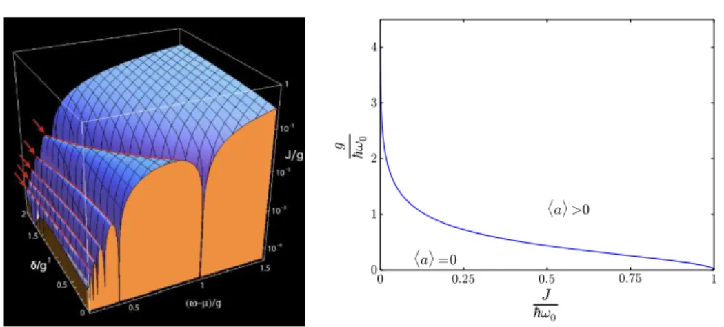
the transverse field is renormalized by a Franck-Condon like exponential factor while the exchange not. In Ref. [53], the authors considered the effect of photon losses on the phase boundary. Interestingly, photon losses favours the disordered trivial phase and the phase boundary shows a tip structure above which the critical coupling Jc
Figure 1.6: Left: Mean-field phase boundary of the Jaynes-Cummings lattice model as a function of effective chemical potential (µef f − ~!0) (we take ~ = 1 for the axis
label) and atom-resonator detuning δ/g. Figure from Ref. [35]. Right: Transition line for ∆/!0 = 0.1 in the case of the Rabi-Hubbard lattice. It reproduces the results of
Ref. [51, 52].
and small g/(~!0).
We have seen in this section that circuit QED setup permits to emulate quantum many-body physics with light. In the same perspective, recent interest have turned to the realization of quantum impurity models, describing discrete local quantum degrees of freedom coupled to continuous baths of excitations. They were originally introduced for the description of magnetic impurities in metals. These models are also relevant for describing transport through quantum dots coupled to metallic leads. Some models of this kind are not integrable and necessitate complex many-body techniques understand their properties. Upon variation of a control parameter, such models may exhibit a quantum phase transition where order is destroyed only by quantum fluctuations. One paradigmatic model of this kind is the spinboson model, initially introduced to describe dissipation.
II
Ohmic spinboson model
Quantum mechanical problems of interest involving a (effective) two-level system are widespread in physics and chemistry. We have seen above the example of the Rabi Hamiltonian, describing transitions between two energy levels of an atom. Other examples include the description of a nucleus of spin 1/2 (with applications in NMR), or the inversion resonance of the ammonia molecule. Such two-level systems can be described by an Hamiltonian of the form,
HT LS= ∆
2σ
x+✏
2σ
where ✏ denotes the energy difference between the two levels and ∆ is the tunneling amplitude between these states.
II.1
Modelling of dissipation
In many cases of interest, the description of the system solely in terms of a two-level system is inaccurate. In practise for a real experiment, the two-level system indeed in-teracts with its surrounding environment through a term of the formP⌫2{x,y,z}σ⌫Ω
⌫,
where Ω⌫ for ⌫ 2 {x, y, z} are environment operators. In the following we will focus
on cases where the coupling is non-zero only along one direction, let us say the z-direction. Provided that the coupling to the environment is sufficiently weak, it is relevant to describe it as a set of harmonic oscillators with a coupling linear in the os-cillator coordinates [54, 55]. In the following and for the remaining of the manuscript, we will take the convention ~ = 1. We reach the spinboson Hamiltonian,
HSB= ∆ 2σ x+✏ 2σ z+ σzX k λk 2 (bk+ b † k) + X k !k ✓ b†kbk+ 1 2 ◆ , (1.48)
where bk (b†k) is the annihilation (creation) operator of a boson in mode k with
fre-quency !k. The spin-bath interaction is fully characterized by the spectral function
J(!) = ⇡Pkλ2
kδ(! − !k). We will assume that J is a smooth function of !, of the
form J(!) = 2⇡↵!s!1−s c exp ✓ −! !c ◆ , (1.49)
where !cis a high frequency cutoff such that ∆ ⌧ !cand the dimensionless parameter
↵quantifies the strength of the coupling. A case of particular interest corresponds to the so-called ohmic coupling which corresponds to s = 1.
II.2
Quantum phase transition and relation with Kondo model
The interaction with the bath plays an important role and affects both the equilibrium and the dynamical properties of the system. In this section, we focus on the ohmic spinboson model and investigate how the interaction with the bath triggers at high coupling a quantum phase transition from a delocalized to a localized phase, in relation to Kondo physics.II.2.a Polaron ansatz and quantum phase transition
To understand better spin-bath effects, let us start by considering the limit ✏ = ∆ = 0. The model reduces then to a set of harmonic oscillators with finite displacements, exactly as considered in Sec. I.2.c. When ∆ 6= 0, the high frequency modes of the bath (!k 4 ∆) could be treated in the adiabatic approximation fashion developped
in Sec. I.2.c. For low frequency modes (!k ∆), the situation is however different
and the term ∆/2σxcannot be treated in a perturbative manner. We therefore follow
Ref. [56] (and references therein) and use a multi-mode coherent state ansatz for the ground state wavefunction,
| vari =
1 p
2[| "zi|fi − | #zi| − fii] , (1.50) where |fi = exph−Pkfk(b†k− bk)
i
|0i (|0i corresponds to the vacuum for all the oscillators). With this ansatz we do not specify the amplitude with which a given mode is displaced ab initio, but these coefficients are determined by minimizing the mean energy of the system,
h var|HSB| vari = − ∆ 2 exp " −2X k fk2 # +X k !kfk2− X k λkfk. (1.51)
We then minimize the variational energy @fkh var|HSB| vari = 0 and find the
self-consistent displacements
fk=
λk/2
!k+ ∆ exp [−2Pkfk2]
. (1.52)
We recover the adiabatic displacement λk/(2!k) for bath modes k such as ~!k4 ∆.
On the other hand, the displacement tends to zero for low frequency modes if ∆ > 0. Bath states now “dress” the spin states, which leads to a renormalization of the tunneling element ∆. Let us estimate this renormalized element ∆r.
∆r= ∆ exp −2~1 ˆ 1 0 d! J(!) (! + ∆r/~)2 / )∆r' ∆ exp −↵ ˆ !c ∆r d! ! / (1.53) )∆r' ∆ ✓ ∆ ~!c ◆ α 1−α . (1.54)
We see in particular that ∆r! 0 when ↵ ! 1, indicating that the bath may forbid
tunneling between spin states at sufficiently high coupling. The effect of the bath is then to polarize entirely the spins, by analogy to a ferromagnetic phase. The spin gets trapped in one of the states | "zi or | #zi.
This result sheds light on the mechanism at the origin of the dissipative quantum phase transition induced by the bath, which has been seen directly by applying the Numerical Renormalization Group (NRG) [57–59]. The procedure involves the re-writing of the partition function using a kink gas representation [58], mapping the problem on an Ising chain with long range 1/r2 interactions. More precisely, the
partition function at inverse temperature β reads at ✏ = 0 Z = 1 X m=0 ✓ ∆ 2 ◆2mˆ β 0 ds2m ˆ s2m 0 ds2m−1... ˆ s2 0 ds1Fm[{sj}] . (1.55)
Fm carries the environment influences in the form of “kink” (or charge) interactions
Fm[{sj}] = exp 8 < : 2m X j=2 j−1 X i=1 W (sj− si) 9 = ; , (1.56)
with in the scaling limit ∆/!c⌧ 1,
W (⌧ ) = 2↵ ln β!c ⇡ sin
✓ ⇡⌧ β
◆
This representation allows to derive valid RG equations following Ref. [60], which are equivalent to the ones derived earlier in the case of the anisotropic Kondo model by Anderson Yuval and Hamann [61] and describe a Kosterlitz-Thouless transition. It is also important to note that expression (1.54) for the renormalized tunneling element can also be found using an adiabatic renormalization procedure, developped in Refs. [62, 63].
II.2.b Relation with Kondo model
The dominant contribution to the electrical resistivity in metals comes from the scat-tering of the conduction electrons with lattice vibrations. This scatscat-tering grows with temperature as more and more lattice vibrations are excited. This results in a mono-tonical increase of electrical resistivity with temperature in most metals. A residual temperature-independent resistivity due to the scattering of the electrons with defects may subsist in the very low temperature range.
A resistance minimum as a function of temperature was however observed in a gold sample in 1934 [64]. The solution to this problem was formulated by Jun Kondo in 1964 [65], when he described how certain scattering processes from magnetic impurities could give rise to a resistivity contribution increasing at low temperatures. We present here the anisotropic1Kondo model, which describes the exchange interaction between
a band of non-interacting conduction electrons with one magnetic impurity. The quantum impurity is represented by a spin 1/2 and it is coupled to the condution electrons by an antiferromagnetic exchange coupling. The corresponding Hamiltonian
HK is HK=vF X k,σ kc†k,σck,σ+J? 2 X k,k0 ⇣ c†k"ck0#S−+ c† k#ck0"S +⌘ +Jz 4 S zX k,k0 ⇣ c†k"ck0"− c† k#ck0# ⌘ , (1.58)
where ckσ(c†kσ) is the annihilation (creation) operator of a conduction electron in
mode k with spin σ. We assume a constant density of states ⇢ = (2⇡vF)−1, where
vF is the Fermi velocity. The term in Jz describes scattering of the electrons in
which the spin is conserved while the term in J? describes spin-flip scattering. The equivalence between the two models can be shown through the kink gas representation [57–61, 63, 66], as the partition function for the anisotropic Kondo model reads
ZK = 1 X m=0 ✓ −⇢J?cos2δe 2⌧c ◆2mˆ β−⌧c 0 ds2m ˆ s2m−⌧c 0 ds2m−1... ˆ s2−⌧c 0 ds1 ⇥ exp 8 < : 2 ✓ 1 + 2δe ⇡ ◆2 2m X j>k=1 ln β ⇡⌧c sin✓ ⇡(sj− sk) β ◆/9= ; . (1.59)
where ⌧c = 1/!c and δe = tan−1(−⇡⇢Jz/4). We have a correspondence between Eq.
(1.56) and Eq. (1.59) in the scaling regime, with the identification
⇢J?! ∆/!c (1.60)
(1 + 2δe/⇡)2! ↵. (1.61)
It follows that the localized-delocalized quantum phase transition in the ohmic spin-boson model is equivalent to the ferromagnetic-antiferromagnetic transition in the anistropic Kondo model. The relationship between the ohmic spinboson model and the anisotropic Kondo model is due to the fact that the low-energy electron-hole excitations have a bosonic character and can be interpreted in terms of density fluctu-ations [62]. The equivalence between these two models notably led to the original un-derstanding of the localization phenomenon in the ohmic spinboson model [67,68]. The equivalence between these two models can also be shown through bosonization [69].
The Kondo effect can be considered as an example of asymptotic freedom, i.e., the coupling of electrons and spin becomes weak at high temperatures or high energies. In this respect, it embodies a paradigmatic model of quantum many-body physics and represents the “hydrogen atom” of this field. Being able to engineer either the Kondo model or the ohmic spinboson model in a controllable manner would then provide a new perspective on these effects. We will come back in more details on related Kondo models in quantum dots in Chapter V.
The description of the collision interactions between the atoms can be done using a pseudopotential description and introducing effective coupling parameters g↵βbetween
states ↵ and β 2 {a, b}. The collisional interaction may result in a strong repulsion for atoms in state b. Low energy states of the quantum dot can be coupled to the condensate reservoir by Raman transitions. Altogether, the Hamiltonian describing the system Hsyscan be written,
Hsys= ✓ −δ0+ gab ˆ dx| b(x)|2⇢a(x) ◆ b†b +Ubb 2 b †b†bb + ˆ dxΩ)Ψa(x) b(x)b†+ h.c. * + Ha, (1.65)
where Ψa(x) is the annihilation operator for an atom a at point x, and ⇢a(x) =
Ψ†
a(x)Ψa(x) is the associated density operator. b annihilates a boson in the atomic
quantum dot, with the wavefunction b†(x). δ0 is the Raman detuning. The term
proportional to gab describes collisional interactions between the atoms on the dot
and the reservoir. Ubb quantifies the on-site repulsion between different b atoms on
the dot. The last term describes the laser-induced coupling between the two types. The low-energies excitations of the BEC consist of linear dispersion phonons with linear dispersion ! = vs|q|, where vsis the sound velocity and q is the momentum of the
excitation. For a large number of atoms in the condensate, one can then consider that the atoms b are coupled to a coherent matter wave described in terms of a quantum hydrodynamic Hamiltonian which reads a zero temperature
Ha =1 2 ˆ dx✓ 1 m⇢a|φ| 2(x) +mvs ⇢a Π2(x) ◆ , (1.66)
where ⇢a(x) = ⇢a+ Π(x). The phase φ is canonically conjugated to Π. Hamiltonian
(1.66) can be diagonalized with the introduction of standard phonon operators, leading to Ha = vsPq|q|b†qbq. In the limit of large on-site repulsion Ubb4 ∆, we can restrict
the dynamics to the two lowest energy levels on the atomic quantum dot. After a unitary transformation S = exp[−iσzφ(0)/2], we reach
Hsys= − ∆ 2σ x+X q !qb†qbq+ −δ + X q λq(bq+ b†q) ! σz 2 , (1.67)
where the coupling coefficients λq read
λq = m|q|v 3 s 2V ⇢a /1/2✓ g ab⇢a mv2 s − 1 ◆ . (1.68)
The dispersion relation above permits the realization on an ohmic spectral function. As shown in Ref. [78], one could extend this proposal to an optical lattice and consider
a lattice of well-separated tightly confining trapping potentials, so that atoms in state b cannot hop from one site to the other. Following the same lines as for the one-site case, the interaction with the common bath of harmonic excitations leads to the following Hamiltonian, HMSB= ∆ 2 M X p=1 σxp− X j6=p K|j−p|σjzσpz+ M X p=1 X k λkeikxp ⇣ b†−k+ bk ⌘σpz 2 + X k !kb†kbk. (1.69) where M denotes the number of sites of the lattice. Eq. (1.69) constitutes the M spin version of the ohmic spinboson model. K|j−p| notably depends on the characteristics of the bath and vanishes for gaa= 2gab [78]. Let us now see what are the additional
effects induced by the coupling to a common bath in this multi-spin case with respect to the single-mode case. This can be studied by applying an unitary transformation ˜H = V−1HV on the Hamiltonian (1.69), with V = expn12Pk
PM j=1σjzeikxjλ!kk(bk− b † −k) o . The transformed Hamiltonian reads:
˜ HMSB= M X j=1 ∆ 2 ) σ+jeiΩj+ σ− j e−iΩj * −X j6=p K|j−p|0 σjzσpz+X k !kb†kbk, (1.70) where Ωj= iPk λk !ke ikxj(b k− b†−k) and K|j−p|0 = K|j−p|+↵!c 2 1 1 + !c2(xj−xp)2 v2 s . (1.71)
Note that we recover the renormalization of the tunneling element induced by the bath in this polaron-transformed rewriting. As can be seen from Eq. (1.70) the ex-citation of spin j indeed comes with a simultaneous polarization of the neighboring bath into a coherent state |Ωji = eiΩj|0i. The tunneling energy is thus renormalized
due to this boson-dependent phase. On top of this effects, the bath also engenders in this multi-spin case a strong Ising-type ferromagnetic interaction K0
|j−p| between the
spins j and p, which is mediated by an exchange of bosonic excitations at low wave vectors, as demonstrated in Ref. [78]. We saw in Sec. II.2.a that the critical value ↵c
of the coupling is ↵c = 1. Due to the strong ferromagnetic interaction between the
spins induced by the bath, this critical value decreases with the number M of sites, as confirmed in Refs. [79–81].
We also note that the ohmic spinboson model can be realized in systems of trapped ions, as exposed for example in Ref. [82]. Environment effects in relation with dissipa-tive critical behaviour have also been studied in the transport properties of quantum dot systems of carbon nanotubes coupled to resistive environments [83], emulating tunnel coupled Luttinger liquids [84]. A prediction of this latter model is the ex-istence of resonance peaks of perfect conductance which narrows when temperature decreases; which translates to environmental conductance suppression in the case of tunneling with dissipation [85] (see also Refs. [86–89] which explore the link between
Luttinger liquid physics). We note related experimental progress studying the back-action of the environment on the conductance in a tunable GaAs/Ga(Al)As Quantum Point Contact setup [90].
II.5
Non-equilibrium dynamics and NIBA equation
Several methods were devised to tackle the spin dynamics in the spinboson model. Among them, the well-known Non-Interacting Blip Approximation (NIBA) allows to reach analytical results in the scaling regime characterized by 0 ↵ 1/2 and ∆/!c ⌧ 1. The derivation of NIBA was originally done in Ref. [62] using a path
integral formalism, that we will present in the next chapter. Interestingly, the NIBA equations can also be derived by using a weak-coupling decoupling over Hamiltonian after a unitary transformation as shown in Ref. [91].
Let us focus on the non-equilibrium dynamics for one spin initially in the pure state | "zi, coupled to a bath at equilibrium at zero temperature at time t0. We
compute the Heisenberg equations of motion for the spin operators σz, σ
+and σ−after
having performed the one-spin version of the unitary transformation introduced in the previous subsection. Replacing the equations obtained for the transverse elements in the one obtained for σz, we reach
˙ σz(t) = −∆ 2 2 ˆ t t0
dsσz(s)heiΩ(t)e−iΩ(s)+ e−iΩ(t)e+iΩ(s)i. (1.72) As σz commutes with the unitary transformation, one can equally compute its
evo-lution in the two frames. To recover equations of NIBA derived in Ref. [62], Dekker decoupled spin and bath expectation values and assumed that the time evolution of the bath operators was governed by the free bath Hamiltonian [91]. This leads to
h ˙σz(t)i + ˆ t t0 dsf (t − s)hσz(s)i = 0, (1.73) where f (t) = ∆2cos 1 ⇡ ˆ 1 0 d!J(!) !2 sin !t / exp −⇡1 ˆ 1 0 d!J(!) !2 (1 − cos !t) / . (1.74) Eq. (1.73) can then be solved exactly using Laplace transformation. One finds that h ˙σz(t)i is the sum of a coherent term p
coh(t) and an incoherent term pinc(t) where
pcoh(t) =
1 1 − ↵e
−γtcosΓt. (1.75)
The oscillation frequency and the decay rate are characterized by Γ/γ = cot[⇡↵/(2 − 2↵)] while the incoherent behavior dominates the long-time dynamics as it behaves as (∆rt)2−2↵. This incoherent behavior is considered to be an incorrect prediction of
In this chapter, we introduced the Rabi model and the Spinboson model, and their relevance for modern experimental techniques. We have also seen the need to de-velop new techniques to tackle the non-equilibirum dynamics in these problems. A particular case of interest related to the Rabi case consists in the developement of a numerical/theoretical framework which would allow to take into account drive and dissipation effects. For the spinboson model, the free dynamics at strong coupling is already a challenge1.
CHAPTER
2
SSE equation and applications
In this chapter, we introduce the stochastic Schr¨odinger equation applicable to Spin-boson models. We consider first a spin 1/2 interacting with a Spin-bosonic bath, described by the Hamiltonian H = ∆2σx+ σzX k λk 2 (bk+ b † k) + X k !kb†kbk. (2.1)
The coupling between the spin and the bosonic bath is characterized by the spectral function2 J(!) = ⇡P
kλ2kδ(! − !k).
In the case of a continuous spectral function, computing the spin dynamics is gen-erally a challenging task and a very large number of different methods were devised to this end. At very weak coupling, Markovian master equations permits to capture qualitatively relaxation and dephasing effects [50, 92]. At higher spin-bath coupling, the influence of the environment on the dynamics becomes more subtle and memory effects have to be taken into account.
As Hamiltonian (2.1) is quadratic in terms of bosonic operators, one can integrate out exactly these degrees of freedom in a path integral approach. This technique was pioneered by Feynman and Vernon [93], and constitutes the starting point of the well-controlled Non Interacting Blip Approximation (NIBA) [62,63] and extensions to it [94–97]. Despite great success in the delocalized phase for ↵ < 1/2, this approxima-tion is for example unable to describe the quantum phase transiapproxima-tion occuring in the ohmic case (see Sec. II.2).
Numerous analytical and numerical methods were built from the Feynman-Vernon influence functional and the “Blip” and “Sojourn” development at the origin of NIBA. This includes stochastic Liouville equations [98–101], Non-Markovian master equations [102, 103], real-time Path Integral Monte Carlo methods [104–107], Quasi-Adiabatic Propagator Path Integral techniques [108, 109] and the Stochastic Schr¨odinger
tion under consideration.
Different approaches following a different path were also devised to tackle the real-time dynamics in this problem, with for example quantum jumps approaches on the wavefunction (or stochastic wavefunction approaches) [110–112]. More recently, vari-ous Numerical Renormalization Group (NRG) techniques [88, 113–121], or Multilayer multiconfiguration time dependent Hartree method [122] were also developped.
We present here the details of the Stochastic Schr¨odinger Equation method, fol-lowing our Ref. [123], and we will try to highlight the links with the other method-s/approaches mentionned above along the derivation.
I
SSE Equation in the case of one spin
A state of the system is described by a wavefunction | i, which belongs to the Hilbert space ✏ = ✏S⌦ ✏B, which is the tensor product of spin and bath spaces ✏S and ✏B. This
mixed spin-boson system is conveniently described in terms of density operators, or density matrices. Considering our quantum system, there is a unique operator ⇢ such that
hAi = tr (⇢A) , (2.2)
for all observable operator A. This operator ⇢ is called the density operator, or density matrix, of the system. We are mainly interested in the dynamics of the spin observ-ables, and the effect of the bath on their dynamics. It is then convenient to define reduced density operators ⇢S and ⇢B as partial traces of the total density matrix
⇢S = tr✏B(⇢) , (2.3)
⇢B= tr✏S(⇢) . (2.4)
We are interested in the time-evolution of the spin-reduced density matrix ⇢S(t) for t ≥ t0, where t0 denotes the initial time. We assume factorizing initial conditions
⇢(t0) = ⇢B(t0) ⌦ ⇢S(t0), with the bath in a thermal state at inverse temperature β.
Stochastic Schr¨odinger Equation for one spin
The elements of the spin-reduced density matrix at time t ≥ t0 are given by
[⇢S(t)]ij = hΣij|Φ(t)i, (2.5)
where the overline denotes a stochastic average and |Φi is the four-dimensional vector solution of the Stochastic Schr¨odinger-like differential equation (2.6),
i@t|Φi = V (t)|Φi, (2.6) with |Φ(t0)i = ) [⇢S(t0)]11ek(t0), [⇢S(t0)]12eh(t0), [⇢S(t0)]21e−h(t0), [⇢S(t0)]22e−k(t0) *T . In Eq. (2.6), we have V = 0 B B @ 0 e−h+k −eh+k 0 eh−k 0 0 −eh+k −e−h−k 0 0 e−h+k 0 −e−h−k eh−k 0 1 C C A. (2.7)
h and k are two complex gaussian random fields with correlations h(t)h(s) =1
⇡Q2(t − s) + l1, (2.8)
k(t)k(s) = l2, (2.9)
h(t)k(s) =i
⇡Q1(t − s)✓(t − s) + l3, (2.10) where lj for j 2 {1, 2, 3} are arbitrary complex constants and
Q1(t) = ˆ 1 0 d!J(!) !2 sin !t, (2.11) Q2(t) = ˆ 1 0 d!J(!) !2 (1 − cos !t) coth β! 2 . (2.12) Vectors hΣij| read hΣ11| = (e−k(t), 0, 0, 0); hΣ12| = (0, e−h(t), 0, 0); hΣ21| = (0, 0, eh(t), 0); hΣ 22| = (0, 0, 0, ek(t)).
The derivation of this result is based on different results related to Refs. [62,63,93, 123–125], which will be exposed below, and can be decomposed into three consecutive steps:
• Integration of the bosonic degrees of freedom in a path integral formalism [93]. This integration will induce spin-spin interactions, which are long range in time. • Rewriting of the spin path in the language of “Blips” and “Sojourns”, following
the work of Ref. [62].
this spin-spin interaction thanks to the introduction of stochastic degrees of freedom [98, 99, 123–125].
I.1
Feynman-Vernon influence functional
Hamiltonian (2.1) is quadratic in terms of bosonic operators, which enables us to carry out an exact integration of these degrees of freedom in a path integral approach. This operation typically generates additional spin-spin interactions in time, whose kernel depends on the spectral properties of the bath. This technique was originally introduced by Feynman and Vernon in Ref. [93] with an integration over extended coordinates of the harmonic oscillators (see also Ref. [63]). One can also derive the result using a coherent-state path integral description. This derivation is done in Appendix A, and we only reproduce the main steps here. Let {|ui} be the basis of coherent states of ✏B, and {|σki} = {| "zi, | #zi} the canonical basis associated with
the z-axis of ✏S. The starting point is to express the density matrix ⇢S in terms of the
evolution operator of the whole system U (t, t0),
⇢S(t) = tr✏B
⇥
U (t, t0)⇢(t0)U†(t, t0)*]. (2.13)
We insert then resolutions of the identity in terms of coherent-state and spin projectors
I=X
k
ˆ
dµ(v)|v, σkihv, σk|, (2.14)
on both sides of ⇢(t0) in the expression (2.13). The coherent state measure is defined
by
dµ(u) = 1
⇡duxduye
−|u|2
, (2.15)
with uxand uy respectively the real and imaginary part of u. The main idea is then
to re-express the forward and backward propagators in terms of integrals over bosonic fields and real-valued spin fields, following the standard path integration procedure. The resulting action of each propagator can be expressed1 in terms of a time-integral
of a Lagrangian L which has only linear and square dependence on the bosonic tra-jectories k and k⇤. Each action can thus be evaluated in an exact manner by means
of the stationary phase condition, d d⌧ @L @ ˙k = @L @ k , (2.16) d d⌧ @L @ ˙⇤ k = @L @ ⇤ k , (2.17)
with well-determined boundary conditions. A final integration over the endpoints of the trajectories give the final result that we summarize below.
At a given time t ≥ t0 and for any |σfi, |σf0i 2 {|σ1i ⌘ | "zi, |σ2i ⌘ | #zi}, the
element of the spin-reduced density matrix between |σfi and |σf0i read
hσf|⇢S(t)|σf0i =
X
k,k0
[⇢S(t0)]k,k0Jk,k0,f,f0, (2.18)
where Jk,k0,f,f0 takes the form
Jk,k0,f,f0 =
ˆ
D[Σ]D[Σ0]A[Σ]A⇤[Σ0]F[Σ, Σ0]. (2.19) The integration in Eq. (2.19) runs over all constant by parts paths Σ and Σ0taking
val-ues in {−1, 1} with endpoints verifying σz|σ
ki = Σ(t0)|σki and σz|σk0i = Σ0(t0)|σk0i,
σz|σ
fi = Σ(t)|σfi and σz|σf0i = Σ0(t)|σf0i. The term A[Σ] denotes the amplitude to
follow one given path Σ in the sole presence of the spin Hamiltonian. The effect of the environment is fully contained in the so-called Feynman-Vernon influence functional F[Σ, Σ0] which reads [93] : F[Σ, Σ0] = e n −1 π ´t t0ds ´s t0ds0 h −iL1(s−s0)Σ(s)−Σ0(s)2 Σ(s0 )+Σ0 (s0 ) 2 +L2(s−s0)Σ(s)−Σ0(s)2 Σ(s0 )−Σ0(s0) 2 io . (2.20) The functions L1 and L2 read
L1(t) = ˆ 1 0 d!J(!) sin !t, L2(t) = ˆ 1 0 d!J(!) cos !t cothβ! 2 . (2.21)
From Eq. (2.20), we see that the bosonic environment couples the symmetric and anti-symmetric spin paths
⌘(t) =1 2[Σ(t) + Σ 0(t)], (2.22) ⇠(t) = 1 2[Σ(t) − Σ 0(t)], (2.23)
at different times. These variables take values in {−1, 0, +1} and are the equivalent of the classical and quantum variables in the Schwinger-Keldysh representation. We have then integrated out the bosonic degrees of freedom, which no longer appear in the expression of the spin dynamics, but the prize to pay is the introduction of a spin-spin interaction term which is not local in time. Dealing with such terms is difficult at a general level. The spin dynamics at a given time t depends on its state at previous times s < t: the dynamics is said to be non-Markovian. The effective action is reminis-cent of the classical spin chains with long-range interaction, where time now replaces space. In particular for an ohmic spectral density given by (1.49), L2(t) / 1/(!ct)2at
long times. When integrated twice, we recover the characteristic ln behavior found by Anderson, Yuval and Hamman [61] when studying the Kondo problem (see II.2.b).