Open Archive TOULOUSE Archive Ouverte (OATAO)
OATAO is an open access repository that collects the work of Toulouse researchers and
makes it freely available over the web where possible.
This is an author-deposited version published in :
http://oatao.univ-toulouse.fr/
Eprints ID : 19577
To link to this article :
DOI: 10.1016/j.ces.2017.07.007
URL :
http://dx.doi.org/10.1016/j.ces.2017.07.007
To cite this version :
Shcherbakova, Nataliya and Rodriguez-Donis, Ivonne
and Abildskov, Jens and Gerbaud, Vincent A Novel Method for Detecting
and Computing Univolatility Curves in Ternary Mixtures. (2017) Chemical
Engineering Science, vol. 173. pp. 21-36. ISSN 0009-2509
Any correspondence concerning this service should be sent to the repository
administrator:
[email protected]
A novel method for detecting and computing univolatility curves in
ternary mixtures
Nataliya Shcherbakova
a, Ivonne Rodriguez-Donis
b,⇑, Jens Abildskov
b, Vincent Gerbaud
caLaboratoire de Génie Chimique, Université Paul Sabatier – INP ENSIACET, 4, allée Emile Monso, 31432 Toulouse, France b
CAPEC-PROCESS, Department of Chemical and Biochemical Engineering, Technical University of Denmark, Building 229, DK-2800 Kgs. Lyngby, Denmark c
Laboratoire de Génie Chimique, CNRS, 4, allée Emile Monso, CS 84234, 31432 Toulouse, France
h i g h l i g h t s
!3D generalized univolatility surfaces are defined.
!Ternary RCM univolatility curves are the loci of relative composition critical points. !Ordinary differential equations describe the univolatility curves.
!A new algorithm based on an initial value problem is proposed. !The method finds univolatility curves not connected to any azeotrope.
Keywords: Residue curve maps Univolatility curves
Homogenous ternary mixtures Differential continuation method Azeotropes bifurcation
a b s t r a c t
Residue curve maps (RCMs) and univolatility curves are crucial tools for analysis and design of distillation processes. Even in the case of ternary mixtures, the topology of these maps is highly non-trivial. We pro-pose a novel method allowing detection and computation of univolatility curves in homogeneous ternary mixtures independently of the presence of azeotropes, which is particularly important in the case of zeo-tropic mixtures. The method is based on the analysis of the geometry of the boiling temperature surface constrained by the univolatility condition. The introduced concepts of the generalized univolatility and unidistribution curves in the three dimensional composition – temperature state space lead to a simple and efficient algorithm of computation of the univolatility curves. Two peculiar ternary systems, namely diethylamine – chloroform – methanol and hexane – benzene – hexafluorobenzene are used for illustra-tion. When varying pressure, tangential azeotropy, bi-ternary azeotropy, saddle-node ternary azeotrope, and bi-binary azeotropy are identified. Moreover, rare univolatility curves starting and ending on the same binary side are found. In both examples, a distinctive crossing shape of the univolatility curve appears as a consequence of the existence of a common tangent point between the three dimensional univolatility hypersurface and the boiling temperature surface.
1. Introduction
Separation of liquid mixtures is one of the most important tasks in the process industry where distillation is the most widely used technique. Remarkably, almost every product on the market con-tains chemicals that have undergone distillation (Kiss, 2014). Beyond conventional distillation of binary and multi-component mixtures, several additional distillation techniques are developed for breaking azeotropes or separating close boiling mixtures: pres-sure swing distillation, azeotropic and extractive distillation. These
techniques are covered at length in several textbooks and reviews (Skiborowski et al., 2014; Gerbaud and Rodriguez-Donis, 2014; Arlt, 2014; Olujic, 2014).
Preliminary conceptual design of distillation processes is based on the knowledge of the mixture thermodynamics and on the anal-ysis of the residue curve maps (RCMs). RCMs are useful to assess the feasibility of splits since they approximate the column compo-sition profiles under total reflux (Doherty and Malone, 2001; Petlyuk, 2004). RCMs also display azeotropes and distillation boundaries, as well as unidistribution and univolatility manifolds. These geometrical concepts have been reviewed in several works. Particularly, the review paper ofKiva et al. (2003)provides a com-prehensive historical review of RCMs mainly taking into account ⇑ Corresponding author.
the Serafimov’s classification of 26 RCM diagrams of ternary sys-tems (Hilmen et al.,2002). The important role of RCMs, unidistribu-tion and univolatility manifolds has been well described by Widagdo and Seider (1996), Ji and Liu (2007), Skiborowski et al. (2014) for azeotropic distillation process design and by Rodriguez-Donis et al. (2009a, 2009b, 2012a, 2012b), Luyben and Chien (2010) and Petlyuk et al. (2015)for extractive distillation design purposes. Noteworthy, the existence and the position of the univolatility curve, a particular type of isovolatility curve, determine the component to be drawn as distillate as well as the configuration of the extractive distillation column.
Isovolatility curves are curves along which the relative volatility of a pair of species is constant:
a
ij¼ yi=xiyj=xj¼ constant; i – j
Along univolatility curves
a
ij¼ 1. As their properties are closelyrelated to those of residue curves (Kiva et al., 2003), univolatility, isovolatility, and isodistribution curves are useful for studying the feasibility of distillation processes. For example, the most vola-tile component is likely to be recovered in the distillate stream with the so-called direct split whereas the least volatile is likely to be in the bottom stream with the so-called indirect split. In azeotropic and extractive distillation processes an entrainer is added to the liquid mixture to be separated, in order to enhance the relative volatility between the components. If the isovolatility rate increases towards the entrainer vertex, it is a good indicator of an easy separation (Laroche et al., 1991; Wahnschafft and Westerberg, 1993; Luyben and Chien, 2010). Furthermore in extractive distillation, the location of the univolatility curve and its intersection with the composition triangle edge determine the component to be withdrawn as a distillate product from the extractive column as well as the proper column configuration (Laroche et al., 1991; Lelkes et al., 1998; Gerbaud and Rodriguez-Donis, 2014).
As shown by Kiva and Serafimov (1973), univolatility curves divide the composition space, X, into different K-order regions. Zhvanetskii et al. (1988)proposed the main principles describing all theoretically possible structures of univolatility curves for zeo-tropic ternary mixtures and their respective location according to the thermodynamic relationship between the distribution coeffi-cients of the light component i, the intermediate j and the heavy component m. 33 possible structures of univolatility curves were reported under the assumption that for every pair of components there exists only one univolatility curve. In the succeeding paper from the same group (Reshetov et al., 1990), the classification was refined by introducing the following nomenclature:
–
a
i;j: an arc shape univolatility curve whose terminal pointsbelong to the same binary side of the composition triangle; –
a
i;j: the univolatility curve connecting two different binary sidesof the composition triangle.
LaterReshetov and Kravchenko (2010) extended their earlier analysis to ternary mixtures having at least one binary azeotrope. Their main observations are:
(a) more than one univolatility curve having the same compo-nent index ‘‘i; j” can appear in a ternary diagram;
(b) the univolatility curve that does not start at the binary azeo-trope can be either
a
i;jora
i;jtype. Ana
i;jcurve can cross aseparation boundary of the RCM;
(c) a ternary azeotrope can be crossed by any type of univolatil-ity curve;
(d) if two univolatility curves intersect at some point, this point is a tangential binary azeotrope or a ternary azeotrope. In both cases there is a third univolatility curve of complemen-tary type passing through this point;
(e) transitions from
a
i;jtoa
i;j(or vice versa) can occur asuni-volatility curves depend on pressure and temperature of vapor – liquid equilibrium (VLE).
Despite the increasing application of univolatility curves in con-ceptual design, there still lacks a method allowing:
(1) detection of the existence of univolatility curves indepen-dently of the presence of azeotropes, which is particularly important in the case of zeotropic mixtures;
(2) simple and efficient computation of univolatility curves. In fact, numerical methods available in most chemical process simulators allow mainly the computation of the univolatility curves linked to azeotropic compositions. Missing univolatility curves not connected to azeotropes will result in improper design of the extractive distillation process. This problem can be solved by a fully iterative searching in the ternary composition space provid-ing the composition values with equal relative volatility (Bogdanov and Kiva, 1977).Skiborowski et al. (2016)have recently proposed a method to detect the starting point of the univolatility curve. They locate all pinch branches that bifurcate when moving from the pure component vertex along the corresponding binary sides. The robustness of this approach to handle complex cases, such as bia-zeotropy when more than one univolatility curve ends on the same binary side, is well demonstrated. Their algorithm is based on MESH equations, including mass and energy balances, summation constraints, and equilibrium conditions.
A less tedious and less time-consuming method is proposed in this paper. It is based on the geometry of the boiling temperature surface constrained by the univolatility condition. This approach will also require the computation of starting binary compositions independently of the azeotrope condition. Such starting points can be easily computed with a vapor-liquid equilibrium model by using the intersections of the distribution coefficient curves on each binary side of the ternary diagram (Kiva et al., 2003).
This paper is organized as follows: First, we revisit the proper-ties of the univolatility curves in RCMs, and prove that they are formed by critical points of the relative compositions. Then, we show that the topology of unidistribution and univolatility curves follows from both the global geometrical structure of the boiling temperature surface and the univolatility condition considered in the full three-dimensional composition - temperature state space. Such a consideration leads to a simple algorithm for the numerical computation of the univolatility curves and other similar objects by solving a system of ordinary differential equations. The starting points of the univolatility curves computation can be detected from the relationship between the distribution coefficients related to the binary pair ‘‘i; j”: the binary distribution coefficients ki;ji , ki;jj and the ternary coefficient k1i;j
m describing the ternary mixture with
the third component ‘‘m” at infinite dilution. Finally, we illustrate our approach by considering several topological configurations of RCM for two distinctive ternary mixtures (thermodynamic model parameters for both mixtures are available online as the supple-mentary materialto this article). The ternary mixture diethylamine – chloroform – methanol at different pressures has two univolatility curves with the same component index ‘‘i; j” and one univolatility curve of type
a
i;j. We also applied our methodto the well-known (though uncommon) case of the binary mixture benzene – hexafluorobenzene exhibiting two azeotropes at
atmospheric pressure. Considering hexane as the third component of the ternary mixture, we trace out the transformation of the type of the univolatility curve from
a
i;jtoa
i;jwith the variation ofpres-sure. The transformation of the topological structure of the uni-volatility curves is properly computed by using the new computational method.
2. Methodology
2.1. Basic definitions and notations
Consider an open evaporation of a homogeneous ternary mix-ture at thermodynamic equilibrium of the vapor and liquid phases at constant pressure. Let xi; yi; i¼ 1; 2; 3 denote the mole fractions
in the liquid and in the vapor phases. T is the absolute temperature of the mixture. Since x1þ x2þ x3¼ 1, only two mole fractions are
independent. Selecting (arbitrarily) x1and x2, the possible
compo-sitions of the liquid belong to the Gibbs triangle
X¼ fðx1; x2Þ : xi2 ½0; 1*; i ¼ 1; 2g, and we denote by @Xits bound-ary. In what follows we will use the vector notation "x ¼ ðx1; x2Þ.
According to the phase rule - in the absence of chemical reactions - a two-phase ternary mixture has three independent state vari-ables. If we select x1, x2and T, the complete state space of a ternary
mixture is the set
fð"x; TÞ : T 2 ½Tmin; Tmax*; "x 2
X
; i ¼ 1; 2gHere Tmin; Tmaxare the minimum and maximum boiling
temper-atures of the mixture. Throughout this paper we assume the vapor phase ideality, i.e. at constant pressure the vapor phase is related to the liquid phase through an appropriate thermodynamic model of the form yi¼ Kiðx1; x2; TÞxi; i¼ 1; 2; 3. The functions Kiare the
distribution coefficients. The liquid mixture of a given composition "x has a corresponding boiling temperature, which can be computed from the thermodynamic equilibrium equation:
U
ðx1; x2; TÞ ¼X 3 i¼1 yi, 1 ¼ X3 i¼1 Kiðx1; x2; TÞxi, 1 ¼ 0 ð1Þ The boiling temperature surface, defined by Eq.(1), can be inter-preted geometrically as a hypersurface in three-dimensional space. We will denote it by W. In a homogeneous mixture each composi-tion of the liquid phase is characterized by an unique value of T, so@Uð"x;TÞ
@T –0 for any T 2 ½Tmin; Tmax* and "x 2X. This allows application
of the Implicit Function Theorem (Lang, 1987) to solve Eq. (1). Thus, in principle, the boiling temperature can be computed as a function of the composition: T ¼ Tbðx1; x2Þ. Hence, in the three
dimensional state space the boiling temperature surface can be represented as a graph of the function Tbðx1; x2Þ. Moreover, by
con-struction,Uðx1; x2; Tbðx1; x2ÞÞ - 0, so the gradient of the function
Tbðx1; x2Þ can be computed explicitly:
@Tb @x1 ¼ , @U @x1 @U @T ; @Tb @x2 ¼ , @U @x2 @U @T ð2Þ
In the standard equilibrium model of open evaporation, a mul-ticomponent liquid mixture is vaporized in a still in such a way that the vapor is continuously evacuated from the system. Tran-sient mass balances imply
_xi¼ xi, yiðx1; x2; TÞ; i ¼ 1; 2; ð3Þ the derivatives in Eq.(3)is computed with respect to some dimen-sionless parameter n (Doherty and Malone, 2001). The solutions of the system of DAEs (1) + (3) define certain curves on the boiling temperature surface W, whose projections onXare called the resi-due curves. The complete set of such curves forms the RCM.
The right hand sides of (3) define a vector field "
v
¼ ðx1, y1; x2, y2Þ in X referred as the equilibrium vector field.
Its singular points describe the pure components and the azeo-tropes of a given mixture. That is, the singular points of the RCM. Below we use the symbol ‘‘^” for the wedge product of two vectors on the plane:
"x ^ "
v
¼v
2x1,v
1x2¼ det x1 x2v
1v
2 " #It is easy to see that the wedge product of two vectors is zero if and only if either at least one of them is a zero vector, or the two vectors are collinear, i.e. "
v
¼ a"x for some scalar a – 0.The relative volatility of component i with respect to component j is given by the ratio
a
ij¼ yi=xi yj=xj¼Ki Kj
If
a
ij> 1, i is more volatile than j and vice versa. The univolatilitycurves are the sets of points inXsatisfying
a
ij¼ 1. The RCM of agiven ternary mixture may contain up to 3 types of
a-curves
defined by their respective indices i, j. Geometrically, these curves are formed by the intersections of the boiling temperature surface, W, with one of the univolatility hypersurfaces defined by equations in the formW
ijð"x; TÞ ¼ Kið"x; TÞ , Kjð"x; TÞ ¼ 0 ð4Þ We will call the solutions to Eqs.(1) and (4), the generalized uni-volatility curves. The uniuni-volatility curves are the projections of the generalized univolatility curves on the ðx1; x2Þ -plane, satisfying forthe relevant pair i-j
wijð"x; Tbð"xÞÞ ¼ Kið"x; Tbð"xÞÞ , Kjð"x; Tbð"xÞÞ ¼ kið"xÞ , kjð"xÞ ¼ 0 ð5Þ Here kið"xÞ ¼ Kið"x; Tbð"xÞÞ denotes the restriction of the i-th
distri-bution coefficient to the boiling temperature surface, W. In what follows we will systematically use uppercase letters for the objects defined in the three-dimensional state space, and lowercase for the corresponding projections onX.
Fig. 1shows the ternary vapor – liquid equilibrium for the mix-ture acetone (x1) – ethyl acetate (x2) – benzene. This mixture forms
no azeotropes. One univolatility curve,
a
2;3¼ 1, between ethylacetate and benzene exists linking the binary edges acetone – ethyl acetate and acetone – benzene. Fig. 1 also shows the mutual arrangement of the boiling temperature surface W and the uni-volatility hypersurface W23 for this zeotropic ternary mixture. The curveHformed by their intersection is the generalized
uni-volatility curve. Its projection (full curve) on the triangular dia-gram,X, is the univolatility curve, here of type
a
2;3, satisfying thethermodynamic condition, w23ð"x; Tbð"xÞÞ ¼ 0. The shape and the
location of univolatility hyper-surfaces are independent of pres-sure, when the vapor phase is an ideal gas. In contrast, the boiling temperature surface W moves up in the three dimensional state space when pressure increases. Its shape can also change. Such a transformation of W can be traced out by considering the transfor-mation of the underlying RCM with pressure variation, as we show in Section 3. The described geometrical picture is essentially related to the ternary mixtures. Indeed, in the higher dimensional case the relation
a
ij¼ 1 describes hypersurfaces in the compositionspaceXinstead of curves. Consequently, the computation method presented below is only valid for ternary mixtures.
The structure of the univolatility curves is closely related to the structure of the unidistribution curves (Kiva et al., 2003), that is the curves inXalong which ki¼ 1 for i = 1, 2, 3. InFig. 1these curves
are represented by dashes. An unidistribution curve is a projection onXof the intersection of the boiling temperature surface, W, with a unidistribution hypersurface defined by Kiðx1; x2; TÞ ¼ 1.
2.2. Unidistribution and univolatility curves in the composition space 2.2.1. The role of distribution coefficients in detecting the existence of the unidistribution and the univolatility curves
If the binary side i-j of the composition triangleXcontains a binary azeotrope, then at this point ki¼ kj¼ 1. Hence this point
belongs to the intersection of a pair of unidistribution curves and to the univolatility curve
a
ij¼ 1. Kiva et al. (2003) highlightedthe relationship between distribution coefficient functions kið"xÞ
of each binary pair, with the presence of unidistribution and the univolatlity curves, using the concept of the distribution coefficient at infinite dilution. More precisely k1i;j
m ¼ limxm!0kmfor m – i; j. We
can compute three functions k1i;jm , ki;ji, and ki;jj for each binary i-j. The last two are the distribution coefficients of the binary system formed by components i and j. Below we use the term distribution curve for the graphs of these functions along binary i-j side of the composition triangle. If, at such a point, both distribution coeffi-cients ki;ji, and k
i;j
j are unity, the point is a binary azeotrope (denoted
Azij) of the mixture ‘‘i; j”. On the other hand, the binary composition
corresponding to the intersection point of a pair of distribution curves k1i;jm and k
i;j i (or k
i;j
jÞ yields the starting point of the
univolatil-ity curve
a
i;m¼ 1 (ora
j;m¼ 1Þ. Similarly, if at some composition ofthe binary i-j the function k1i;jm is unity, this composition initiates
the unidistribution curve of component m.
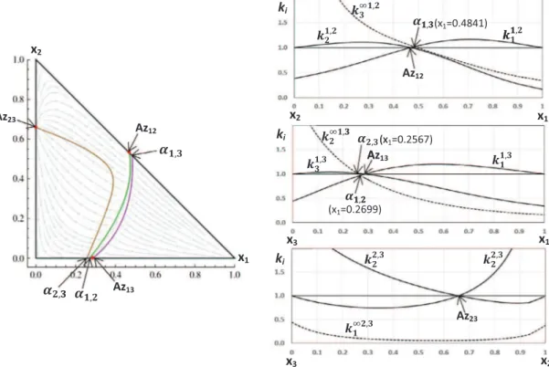
Fig. 2illustrates these concepts for the ternary mixture acetone (1) – chloroform (2) – methanol (3), including the functions k1i;jm ,
ki;ji , and k i;j
j and the univolatility and unidistribution curves.
As shown inFig. 2, each binary pair has a single azeotrope, and there is one ternary azeotrope (saddle type). Each univolatility curve
a
i;jbeginning at the binary i-j azeotrope terminates at thebinary composition corresponding to the intersection of either
(k1m;ji , k m;j j ) or (k 1i;m j , k i;m
i ). In particular, the curve
a
1;2¼ 1 reachesthe edge 1–3 at the intersection of k11;3 2 and k
1;3
1 . The curve
a
1;3¼ 1 reaches the edge 2–3 at the intersection of k12;31 and k 2;3 3 .Similarly, the curve
a
2;3¼ 1 reaches the edge 1–3 at theintersec-tion of k11;3 2 and k
1;3
3 . Thus, all starting points of univolatility and
unidistribution curves can be determined by the computation of the distribution coefficients kið"xÞ in the binaries only. Next, we will
focus on the thermodynamic interpretation of the univolatility curves.
2.2.2. Thermodynamic meaning of the unidistribution and the univolatility curve
Consider a residue curve bðnÞ ¼ ðx1ðnÞ; x2ðnÞÞ inXand the
uni-volatility curve
a
1;2¼ 1. By definition, b is a solution to thediffer-ential equation _"x ¼ "
v
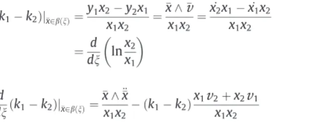
. Moreover, along b the following relations holds ðk1, k2Þj"x2bðnÞ¼ y1x2, y2x1 x1x2 ¼ "x ^ "v
x1x2 ¼ _ x2x1, _x1x2 x1x2 ¼ d dn ln x2 x1 $ % ð6Þ d dnðk1, k2Þj"x2bðnÞ¼ "x ^ €"x x1x2, ðk1, k2Þ x1v
2þ x2v
1 x1x2 ð7ÞThe detailed derivation of equalities (6) and (7) is given in Appendix A.
Suppose the curve b intersects the univolatility curve
a
1;2¼ 1 atsome point "x1¼ bðn1Þ. Then k1ð"x1Þ , k2ð"x1Þ ¼ 0 and at the point "x1
the left-hand side of Eq.(6)vanishes. Since the natural logarithm is a monotonous function, this implies that "x1is the critical point
of the ratio x2=x1along b. In particular, "x1 satisfies the necessary
conditions for the solutions of the constrained optimization prob-lem on the form
min = max "xðnÞ2b
x2ðnÞ x1ðnÞ
Geometrically, this means that the slope of the ray issued from the origin and moving along the residue curve b has an extremum at the point where the residue curve intersects the univolatility curve
a
1;2¼ 1. Since ðk1, k2Þðx1Þ ¼ 0, only the wedge product termremains in Eq.(7). It follows that the function x2ðnÞ=x1ðnÞ has a
local maximum at n1 if "x1^ €"xðn1Þ < 0 and a local minimum if
"x1^ €"xðn1Þ > 0, except at an inflection point where "x1^ €"xðn1Þ ¼ 0.
In the latter case n1corresponds to the inflection point of the ratio
x2ðnÞ=x1ðnÞ.
Recall that the curvature of a curve on a plane is given by
v
¼ _"x ^ €"x_"x
j j
j j3 (Do Carmo, 1976). Comparing Eq. (6) with residue
curves of Eqs.(3) we see that at the point "x1 the vectors "x and
"
v
¼ _"x are collinear, so the type of the extremum is defined by the sign of the curvaturev. The sign of the curvature characterizes
the convexity of the curve. Indeed, when _x1–0, the curve b canbe represented as a graph of the form x2¼ x2ðx1Þ. In this case
v
¼ x00 2ð1 þ ðx02Þ2
Þ,3=2, where ‘‘0” denotes the derivative with respect to x1, and hence
v
> 0 corresponds to convex curves, whilev
< 0corresponds to concave curves. Moreover, residue curves Eq.(3) imply that at the point of intersection with the univolatility curve x0
2¼ x2
x1P0. This means that residue curves intersect the
univolatil-ity curve
a
1;2¼ 1 in the ascending direction (with respect to thechosen pair of axes). All of this remains true for the univolatility curves
a
1;3¼ 1 anda
2;3¼ 1 modulo the initial choice of thecoordi-nate axes. Putting together these arguments, we get the following results:
Theorem 1.
(a) Univolatility curves
a
i;jon the RCM of ternary mixtures are theloci of the critical points of the relative compositions xj=xi.
(b) Along any residue curve, the type of the local extremum of the ratio xj=xiat the point of the intersection with the univolatility
curve
a
i;j¼ 1 is determined by the sign of its curvature at thispoint, with respect to the axes xi, xj: It has a minimum if
v
> 0, and a maximum ifv
< 0.(c) Any residue curve intersecting the univolatility curve
a
i;j¼ 1 atthe point "x1is tangent to the ray x1j=x1i¼ const. It intersects the
univolatility curve in ascending direction with respect to the axes xi; xj. Moreover, if the curvature of this residue curve has
constant sign, the whole curve will entirely lie on the same side of the ray x1j=x1i¼ const.
Remark 1. The geometrical characterization given in property c is well known in the literature (Kiva et al. 2003).
Remark 2. Azeotropes and pure states are singular points for the equilibrium vector field,
v
. Hence, they are asymptotic limits of the residue curves, as n goes to infinity in Eq.(3). In other words, residue curves do not pass through them. Consequently, azeo-tropes and pure states are excluded from the context ofTheorem 1. In order to detect the global extremum value of the relative com-position along a residue curve, one has to consider the asymptotic upper and lower limits associated to straight curves xi=xj¼ constconnecting the pure states to the azeotropes associated with the residue curve under consideration.
The ternary mixture of acetone (1) – chloroform (2) – methanol (3) (shown inFig. 2), has one ternary azeotrope of saddle type and 3 binary azeotropes as nodes. InFig. 3we present the sketch of its
RCM. For the sake of convenience, in the upper right corner we recall the orientation of the axes for the coordinate systems having the origin at different pure states. Azeotropes are indicated by red dots. The three full curves are univolatility curves. Consider first the residue curve b1. Along this curve the ratio x2=x1has a local
minimum at the point P1where it intersects the univolatility curve
a
1;2¼ 1, and at P2(intersection witha
2;3¼ 1Þ the local mimimumvalue of x2=x3 is reached. Along the curve b2 the function x2=x1
has a local maximum at P3(intersection with
a
1;2¼ 1Þ and at P4,x2=x3has local maximum (intersection with
a
2;3¼ 1Þ. Finally, alongb3there is a local minimum of x1=x3at the point P5(intersection
with
a
1;3¼ 1Þ.2.3. Practical computation of the unidistribution and univolatility curves
2.3.1. Detection of the starting points of the unidistribution and the univolatility curves on the binary sides of the composition spaceX
As shown inFig. 1, the existence of the univolatility curves can be detected from the equality of the values of the binary distribu-tion coefficients, including the coefficients of the components at infinite dilution. The formal calculation of the starting points of the univolatility curves relies upon the solution of the algebraic equations(5)restricted to the binary mixtures. Such a restriction means that the kimust be replaced by the appropriate binary
dis-tribution coefficients or the disdis-tribution coefficient at infinite dilu-tion. Eq.(5)describing the univolatility curves are restrictions of Eq.(4)to the boiling temperature surface defined by Eq.(1). Since along the binary side i-j, we have xi¼ 1 , xj and xm¼ 0, this side
can be parametrized by a single composition variable xj. Thus, for
any binary i-j we have to solve the following system of algebraic equations:
Ki;j
iðxj; TÞ , Ki;jj ðxj; TÞ ¼ 0; Ki;jiðxj; TÞð1 , xjÞ þ Ki;jj ðxj; TÞxj¼ 1 ð8:1Þ Ki;j
iðxj; TÞ , K1i;jm ðxj; TÞ ¼ 0; Ki;jiðxj; TÞð1 , xjÞ þ Ki;jj ðxj; TÞxj¼ 1 ð8:2Þ Ki;j
jðxj; TÞ , K1i;jm ðxj; TÞ ¼ 0; Ki;jiðxj; TÞð1 , xjÞ þ Ki;jj ðxj; TÞxj¼ 1 ð8:3Þ
Here, as before, K1i;j
m ¼ limxm!0Km. Thermodynamic models are
needed for the pure component vapor pressures and the activity coefficients of all 3 species i-j-m.
Computation of starting points for the unidistribution curves is completely analogous. But, the first equation in each of the systems (8.1)–(8.3)must be replaced by one of the following equations,
Ki;jiðxj; TÞ ¼ 1; Ki;jj ðxj; TÞ ¼ 1; K1i;jm ðxj; TÞ ¼ 1 ð9Þ The algorithm of the computation of the starting points of the unidistribution and univolatility curves, using Eqs.(8.3) or (9)does not require the existence of binary azeotropes. It is applicable to any zeotropic or azeotropic homogeneous mixture. However, all binary azeotropes, if they exist, will be found as solutions. In the next section we will derive the ordinary differential equation allowing computation of the whole univolatility or unidistribution curve by numerical integration.
2.3.2. The generalized univolatility and unidistribution curves Consider a generalized univolatility curve H:
s
!HðsÞ ¼ðx1ðsÞ; x2ðsÞ; TðsÞÞ in the three-dimensional state space. By
defini-tion,His formed by the intersection of two hypersurfaces defined by the algebraic equations Uðx1; x2; TÞ ¼ 0; Wðx1; x2; TÞ ¼ 0, the Fig. 3. Relationship between univolatility curves and residue curves for the mixture acetone (1) – chloroform (2) – methanol (3).
latter representing any of the Eqs.(4). A short recall about surface geometry is given inAppendix B.
Let U ¼ ðU1; U2; U3Þ denote a tangent vector toHat some point.
By construction, U is orthogonal both to the normal vector Nw¼rUto the boiling temperature surface W and to the normal
N ¼rWto the univolatility hypersurface (seeFig. 1). If the two hyper-surfaces are in general position (i.e. do not have common tangent planes), we have U ¼ Nw4 N, implying
U1¼@
U
@x2 @W
@T, @U
@T @W
@x2 ; U2¼@U
@T @W
@x1 ,@U
@x1 @W
@T; U3¼ @U
@x1 @W
@x2, @U
@x2 @W
@x1 ð10ÞTheorem 2. The generalized univolatility curve projecting on the univolatility curve
a
ij¼ 1 is an integral curve of the vector field U defined by Eq.(10), i.e., it is a solution to the following system of ordinary differential equations in three-dimensional state space:dx1 d
s
¼ @U
@x2 @W
ij @T , @U
@T @W
ij @x2 ; dx2 ds
¼ @U
@T @W
ij @x1 ,@U
@x1 @W
ij @T ; dT ds
¼ @U
@x1 @W
ij @x2 ,@U
@x2 @W
ij @x1 ð11ÞThe geometrical interpretation of Theorem 2is illustrated in Fig. 1.
Remark 3. In principle, the boiling temperature surface and the univolatility hypersurface can have isolated points of common tangency. In this case U1¼ U2¼ U3¼ 0, i.e., the generalized univolatility curve degenerates into a point. Comparing Eqs.(11) and (2), after all necessary simplifications, gives
U3¼ U1 @Tb @x1þ U2
@Tb
@x2; ð12Þ
and therefore any singular point of the univolatility curve on X
obeying U1¼ U2¼ 0 is a singular point of the corresponding
gener-alized univolatility curve and vice versa. Such isolated singular points can be of elliptic or hyperbolic type. In the first case the cor-responding degenerated univolatility curve will just be a point inX,
whereas in the last case it is composed of four branches joining at the singular point. Note that such singular points of univolatility curves are not necessarily singular points of the RCM. Another highly non-generic situation occurs when a curve of
a
ijtype shrinksinto a point on the binary edge of the composition spaceX. Such
point can be either a regular point of the RCM or it can coincide with a tangential binary azeotrope. In the latter case the RCM will have a binary azeotrope which does not generate any univolatility curve that is different from a point. In Section3we provide the examples of these highly non-generic and unusual configurations.
Remark 4. All the above formulae can be directly applied for the computation of the unidistribution curves by setting
Wðx1; x2; TÞ ¼ Kðx1; x2; TÞ , 1, where K is any of the distribution
coefficients.
2.3.3. From three-dimensional model to the numerical computation of the univolatility curves
Eq.(11)provides an effective tool for numerical computation of the univolatility curves using the standard Runge-Kutta schemes for the ODE integration. The initial points for such integration can be computed by finding solutions of Eqs.(8.1)–(8.3)by means
of a standard non-linear equations solver like the Newton-Raphson method. Once the initial point is chosen, the whole generalized univolatility curve can be computed by following the intersection of two associated hyper-surfaces using the vector field U in the direction pointing inside the composition spaceX. In particular, no further iteration procedure is required to compute the uni-volatility curve in the interior points of X. In addition, to avoid
the difficulties associated with possible stiffness of Eqs.(11), it is recommended to rewrite them in the normalized form, which is equivalent to choose the arc length s of the curve as the new parameter of integration instead of
s.
For definiteness, consider the curve
a
i;j¼ 1 starting from the 3–1 binary side, that is, from the x1-axis. The starting point of this
curve is a projection of a point ðx0 1;ij; 0; T
0
1;ijÞ in the state space. The
whole curve
a
i;j¼ 1 can be computed as the projection of thesolu-tion of the following initial value problem:
dx1 ds ¼ dijUij1ðx1; x2; TÞ kUijðx1; x2; TÞk ; dx2 ds ¼ dijUij2ðx1; x2; TÞ kUijðx1; x2; TÞk ; dT ds¼ dijUij3ðx1; x2; TÞ kUijðx1; x2; TÞk ð13Þ x1ð0Þ ¼ x01;ij; x2ð0Þ ¼ 0; Tð0Þ ¼ T01;ij ð14Þ dij¼ sign Uij2 x 0 1;ij; 0; T 0 1;ij & ' & ' ð15Þ
Analogous initial value problems can be formulated for the curves starting from other binary sides of X by an appropriate
modification of the initial conditions(14)and the starting direction (15). Here is the sketch of the general algorithm:
1. Find all starting points of the univolatility curves on each binary side i-j ofXand form the list of all possible starting points by solving Eqs.(8.1)–(8.3).
2. Take the starting points of the list created in point 1 and solve the initial value problem of type(13)–(15)with an appropriate choice of the initial direction. The numerical integration should be continued until one of the following situations occurs: x1< 0; x2h0; x1þ x2i1, i.e. the border ofXis attained. Then stop
integration.
3. Exclude both initial and final points of the curve computed in point 2 from the list of starting points.
4. Go back to point 2 until the list of starting points is exhausted. The advantage of the described algorithm is that once the Eq. (13)is given, we only need to use a standard solver for a pair of non-linear algebraic equations and a standard ODE integrator. The prototype of the algorithm described above was realized in Mathematica 9, and was used in case studies discussed in the next section. The choice of Mathematica 9 is not prohibitive. The algo-rithm can easily be implemented in other scientific computing packages like MATLAB of MAPLE allowing Eq.(13)to be written by symbolic differentiation of the thermodynamic model. The implementation using the standard algorithmic languages is possi-ble by coupling with a compatipossi-ble library of automatic differentiation.
Remark 5. The above method of calculation of the univolatility and unidistribution curves was developed under the ideality assumption of the vapor phase. Although the geometrical deriva-tion remains the same, certain definideriva-tions and computaderiva-tions must be adapted when considering a non-ideal vapor phase. In that case, and in order to correctly define the concept of the univolatility curve in the composition space X, the relations yi¼ Kiðx;"y; TÞxi;
i ¼ 1; 2; 3, need first to be solved with respect to the vapor mole fractions yi. In principle, this is possible thanks to the general Implicit Function Theorem, which also provides the explicit formulae for the derivatives of yi with respect to xi and T. In the presented numerical algorithm, a standard ODE solver needs to be replaced by a DAE solver, allowing to compute the vapor phase at each step of integration.
3. Computation of univolatility curves in ternary mixtures. Case studies
Reshetov and Kravchenko (2007a, 2007b)studied 6400 ternary mixtures including 1350 zeotropic mixtures, corresponding to Ser-afimov class 0.0–1. The structure of the univolatility curves was determined for 788 zeotropic systems, using the Wilson activity coefficient equation based on both, ternary experimental data and reconstructed data of binary mixtures. 15 of the possible 33 classes defined by Zhvanetskii et al. (1988) were found, and 28.4% of computed ternary diagrams exhibited at least one volatility curve indicating the necessity of computing the uni-volatility curve even for zeotropic mixtures. Unfortunately, the authors provided no information on the components used in their analysis. In the case of ternary mixtures with at least one azeo-trope, Reshetov and Kravchenko (2010) extended their earlier study (Reshetov et al. 1990) by considering 5657 ternary mixtures where 30% of all cases were modelled from experimental data. Table 1summarizesReshetov and Kravchenko results (2010)and arranges ternary diagrams into three groups according to the num-ber of
a
i;jcurves of each component pair ‘‘i; j”. We use Serafimov’sclassification instead of Zharov’s classification (see correspondence in Kiva et al., 2003) used in the original paper. According to Table 1, 79.2% of the analysed mixtures had at least one univolatil-ity curve. Among them, 97.2% have only one univolatilunivolatil-ity curve
a
i;jfor each index ‘‘i; j”, while 2.7% involved two univolatility curves
a
i;j. Two ternary diagrams belonging to the Serafimov class(1.0-1a) exhibited three univolatility curves
a
i;jwith the samecompo-nent index ‘‘i; j”. Furthermore, about 2% of studied cases displayed at least one univolatility curve of
a
i;j-type. According to these data,real ternary mixtures exhibiting more than one univolatility curve for a component index ‘‘i; j”, as well as the
a
i;j-type univolatilitycurve are rare at atmospheric pressure. Below we present two
examples with quite an uncommon behavior related to the exis-tence of at least two univolatility curves with the same component index ‘‘i; j” and one univolatility curve belonging to
a
i;j-type. Thefirst example is the ternary mixture diethylamine (1) – chloroform (2) – methanol (3) which was reported in the paper ofReshetov and Kravchenko (2010)as exhibiting two univolatility curves
a
1;2.The second example is the well-known case of the existence of two binary azeotropic mixture for benzene – hexafluorobenzene providing a particular shape of the univolatility curves. The atmo-spheric pressure was selected for defining the initial Serafimov class of the RCM for each case study. The RCMs were computed using NRTL model with Aspen Plus built-in binary interaction parameters. For the binary mixture diethylamine (1) – chloroform (2), the binary coefficients were determined from experimental vapor – liquid equilibrium data (Jordan et al., 1985).
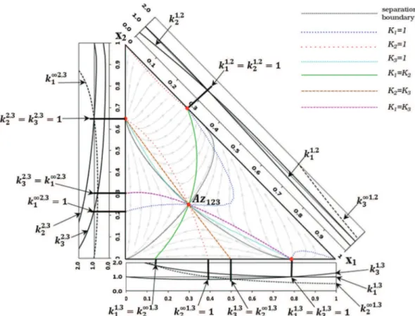
3.1. Case Study: diethylamine (1) – chloroform (2) – methanol (3) InFig. 4we show the RCM of this mixture at 1 atm. It has two binary maximum boiling azeotropic points in the binary edges diethylamine (1) – chloroform (2) and diethylamine (2) – methanol (3), and one binary minimum boiling azeotrope on the edge chlo-roform (2) – methanol (3). The corresponding Serafimov class is 3.0-1b with only 0.9% of occurrence (Hilmen et al., 2002). At 1 atm, there are three univolatility curves of
a
i;j-type coming fromeach binary azeotrope. This is consistent with the behavior of the distribution curves along the binary sides 1–2, 1–3 and 2–3 (right diagrams) and the unity level line. The univolatility curve
a
1;3¼ 1 issued from Az13arrives at the edge 1–2 at the intersectionpoint of the curves k11;23 and k1;21 . Similarly, the curve
a
1;2¼ 1 startsat Az12and reaches the edge 1–3 at the point corresponding to the
intersection of the distribution curves k11;32 and k 1;3
1 , and the curve
a
2;3¼ 1 issued from Az23terminates at the point given by theinter-section of the curves k11;32 and k 1;3
3 . As a consequence of the
differ-ence in nature of the azeotropes and the close boiling temperatures of the components, diethylamine (55.5 "C) – chloroform (61.2 "C) – methanol (64.7 "C), the small variation of the pressure causes a significant transformation of the topological structure of the uni-volatility curves.
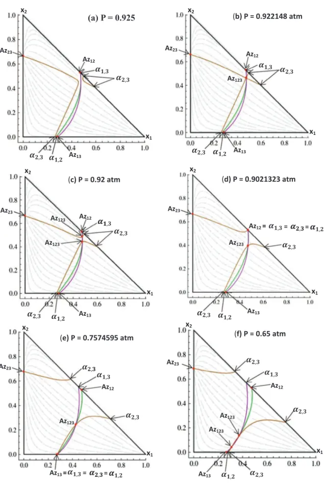
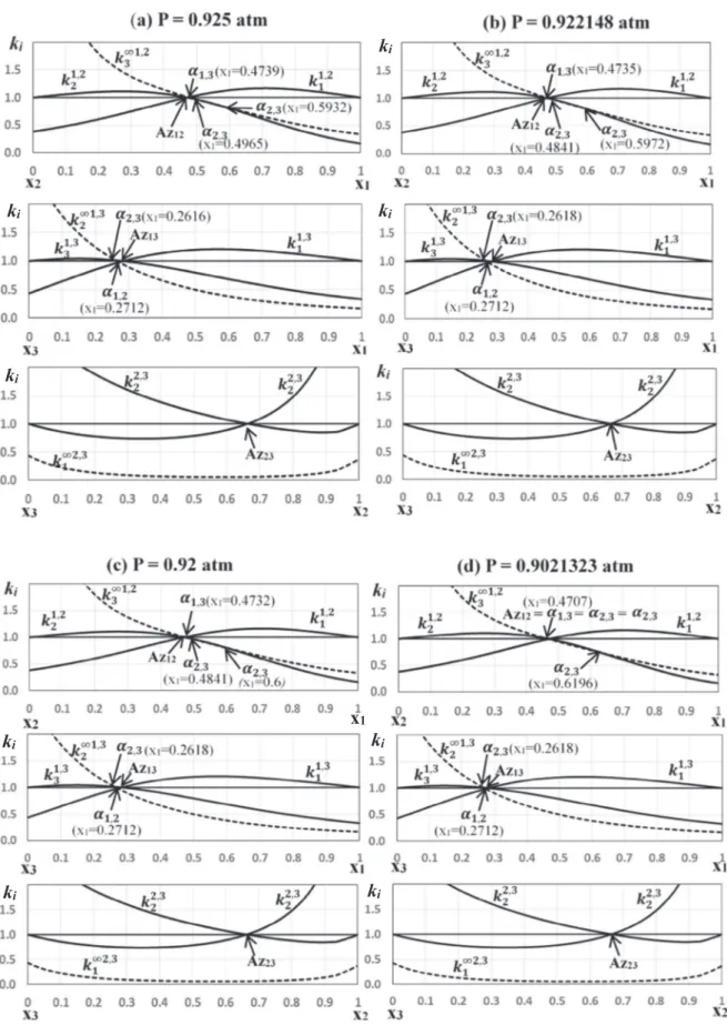
Indeed, as it is shown inFig. 5, changing the pressure to 0.5 atm leads to several bifurcations of the topological structure of RCM
Table 1
Occurrence of univolatility curves having different types in several Serafimov classes of ternary diagrams according to []. adapted fromReshetov and Kravchenko, 2010
Serafimov’s class Oneai;j Twoai;j Threeai;j
ai;j ai;j ai;j ai;j ai;j ai;j
1.0-1a* 1 938 11 29 – 2 1.0-1b* – 49 1 – – – 1.0-2* 19 682 5 15 – – 2.0-1 – 23 – – – – 2.0-2a* – 3 – 2 – – 2.0-2b* 14 1975 3 24 – – 2.0-2c – 63 – 1 – – 3.0-2 – 174 – 10 – – 3.0-1b* – 29 1 2 – – 1.1-2 7 27 5 0 – – 1.1-1a 1 – – – – – 2.1-2b 5 32 – 1 – – 2.1-3b* 10 59 2 5 – – 2.1-3a – 29 – – – – 3.1-2 – 168 – 5 – – 3.1-1b – 2 – – – – 3.1-1a – 2 – – – – 3.1-4* – 47 – – – – * Antipodal structure.
along with the transformation of the structure of both univolatility and distribution curves. First, the pressure is slightly decreased (Fig. 5a) and a new branch of
a
2;3type arises from the edgediethy-lamine (1) – chloroform (2). This new branch is not connected to any azeotropic point. With further pressure decrease, the two uni-volatility curves
a
2;3 anda
2;3 get closer until the first bifurcationappearing at P 8 0.922148 atm (seeFig. 5b): the two branches of the curve
a
2;3¼ 1 meet each other at a singular point. Such asin-gularity resulting from the common tangency between the boiling temperature surface and the univolatility hypersurface was described in Remark 3 in the Section 2.3.2. In the present case the situation is even more interesting because at this singular point the curve
a
2;3¼ 1 intersects the other two univolatility curvesforming a ternary azeotrope Az123 of the saddle-node type. With
decreasing pressure slightly (Fig. 5c) the saddle–node azeotrope splits into a pair of ternary azeotropes: a saddle (the upper one) and a stable node (the lower one). The curve
a
2;3¼ 1 is now formedby two branches of
a
2;3type.With a further decrease of pressure (Fig. 5d) the saddle ternary azeotrope merges with the binary azeotrope diethylamine (1) – chloroform (2) at P 8 0.90212323 atm, forming a transient tangen-tial binary azeotrope. An infinitesimal reduction of the pressure gives rise to a binary azeotrope Az12of saddle type. The resulting
RCM corresponds to the Serafimov class 3.1-1b which has zero occurrence in real mixtures according toHilmen et al. (2002).
The next bifurcation occurs at P 8 0.7574595 atm (Fig. 5e): the three univolatility curves
a
i;j¼ 1 meet each other on the binaryside diethylamine (1) – methanol (3) forming a tangential binary azeotrope Az13. Continued pressure reduction (Fig. 5f) moves the
bottom of the curve
a
2;3¼ 1 to the right inducing the splitting ofthe transient azeotrope into a binary stable node and a new ternary azeotrope of saddle type. We observe again a RCM with 2 ternary azeotropes inFig. 5f: a saddle (in the bottom) and a stable node (in the top) resulting from the double intersection of the three uni-volatility curves of different types. At P 8 0.627963 atm (Fig. 5g),
two ternary azeotropes merge in a single saddle-node ternary azeotrope, which disappears with a further pressure decrease. Below this singular value of pressure and until P = 0.5 atm, the RCM belongs again to Serafimov class 3.0-1b as it was at P = 1 atm. However, the maximum boiling azeotropic mixture diethylamine (1) – methanol (3) is now the stable node type instead of the mixture diethylamine (1) – chloroform (2) at P = 1 atm (Fig. 4). Note, that the resulting two RCMs of Serafimov class 3.0-1b have different topology of univolatility curves. At 0.5 atm there is one curve of type
a
1;3, one curve of typea
1;2andtwo curves of type
a
2;3instead of just one curve of typea
i;jfor eachpair of indices.
Comparing the RCM diagrams inFig. 5 to the corresponding distribution curves inFig. 6, shows that the bifurcation resulting from the intersection of more than one univolatility curves at the binary edges can be detected by the analysis of the intersec-tions of the distribution curves associated with the distribution coefficients k1i;jm , k
i;j i and k
i;j
j. Indeed, inFig. 6a-c andFig. 6f, both
terminal points of the curve
a
2;3¼ 1 with the binary sidediethy-lamine (1) – chloroform (2) correspond to the double intersection of the distribution curves of k11;2
3 and k 1;2
2 . These results show the
efficiency of this criterion for the curves of type
a
i;j. InFig. 6d theexistence of the tangential binary azeotrope Az12on the 1–2 edge
is well in accordance with the common intersection point of the three distribution curves k11;23 , k1;21 and k1;22 . The same behavior can be also observed by comparingFigs. 5e and6e for the binary tangential azeotrope on the edge diethylamine (1) – methanol (3): the three distribution curves k11;3
2 , k 1;3 1 and k
1;3
3 intersect at the
azeotropic composition Az13. The formation (Fig. 5b and g) and
the splitting (Fig. 5c and f) of the saddle-node type ternary azeo-tropes cannot be detected from the behavior of the distribution curves along binary edges. The existence of the ternary azeotropes is detected by the existence of the intersection of at least two uni-volatility curves. ,
Az
23 , ,k
ix
3x
2x
1x
2Az
12Az
23Az
13 , , ,Az
13 , , , (x =0.2567) , (x1=0.2699)x
1x
3A
(x1 ,x
1Az
12x
2 , , , , (x1=0.4841)k
ik
ix
1Az
12Az
23 ,(a) P = 0.925
Az
13 , , ,x
2x
1Az
12Az
23Az
13 , , ,(
b) P = 0.922148 atm
,Az
123x
2x
2x
1Az
13 , , ,(
c) P = 0.92 atm
,Az
12Az
123Az
123Az
23(
d) P = 0.9021323 atm
x
1Az
23Az
13 , , ,Az
123x
2Az
12=
=
,=
,=
,x
2x
1(
e) P = 0.7574595 atm
Az
23Az
12 , , ,Az
13=
=
,=
,=
,(
f) P = 0.65 atm
x
2x
1Az
23Az
12 , , ,Az
13 , ,Az
123Az
123Az
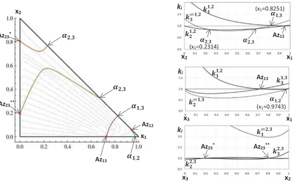
1233.2. Case Study: hexane (1) – benzene (2) – hexafluorobenzene (3) As it is shown inFig. 7, at the reference pressure 1 atm, the RCM of this ternary mixture has two binary azeotropes Az123(saddle) and
Az11
23(stable node) on the binary side benzene (2) –
hexafluorozene (3). The other two binary azeotropes belong to the sides ben-zene (2) – hexane (1) and hexafluorobenben-zene (3) – hexane (1). The RCM is characterized by four univolatility curves issued from each of the binary azeotropes. In addition, the univolatility curve
a
2;3¼ 1 is composed by two branches ofa
i;j– type. As shown inthe right-hand side ofFig. 7, the terminal points of both curves
a
2;3 on the binary edge hexane (1) – benzene (2) can be detectedby the double intersection between the distribution curve of k11;2
3 with the curve for k 1;2
2 . The pair of binary azeotropes on the
2–3 edge comes from the double simultaneous intersection of the distribution curves k2;32 and k2;33 with the unit level curve.
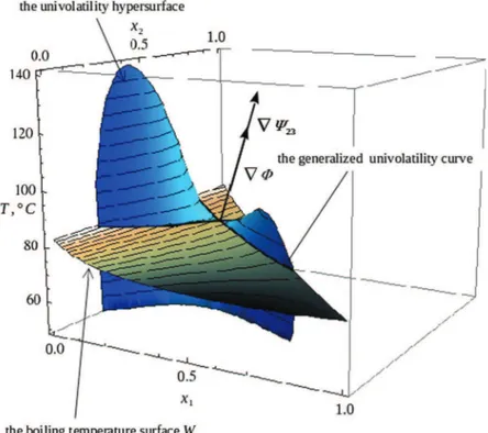
The pressure increase allows tracing out some peculiar transfor-mations of the topological structure of the RCM of this mixture. First of all, at P 8 1.07705 atm, two branches
a
2;3 join to form aunique cross shape univolatility curve, as shown inFig. 8a. A sim-ilar configuration was observed inFig. 5b. This phenomenon corre-sponds to the existence of the common tangent point of the boiling temperature surface and the univolatility hypersurface, as shown inFig. 10. Unlike to the case presented inFig. 5b, here the singular-ity of the univolatilsingular-ity curve is not related to the existence of the ternary azeotrope. In fact, this singular point is not a critical point of the boiling temperature Tb, and hence the boiling temperature
surface W intersects the other two univolatility hypersurfaces
W12¼ 0 andW13¼ 0 far from this point. With the further
incre-ment of pressure (Fig. 8b) the two branches of the curve
a
2;3¼ 1split into two curves of
a
i;j-type. Such a transformation cannot bedetected from the analysis of the distribution curves k1i;jm , ki;ji and ki;jj . Indeed, the distribution curves diagrams at P = 1 atm (Fig. 7) and at P = 1.2 atm (Fig. 9) are almost identical. Remarkably, one of the new univolatility curves (labelled
a
12;3) connects two binary
azeotropes Az123 and Az 11
23. With the further pressure growth, the
binary azeotrope Az12 disappears together with the univolatility
curve
a
1;2¼ 1 and the right branch of the curvea
2;3¼ 1. The twoazeotropes Az1 23and Az
11
23move closer making the curve
a
12;3shorterand closer to the edge 2–3. At P 8 4.93806 atm (Fig. 11) Az1 23and
Az11
23 join to form a singular binary azeotrope, which is not
con-nected to any univolatility curve. This point corresponds to the only common point between the boiling temperature surface and the hypersurface defined byW23¼ 0 in the tree-dimensional state
space. With the further pressure increase, this azeotrope disap-pears and
a
1;3¼ 1 remains the only univolatility curve of thetern-ary mixture. 4. Conclusion
The feasibility of the separation and the design of distillation units can be assessed by the analysis of residue curve maps (RCMs) and univolatility and unidistribution curves. Kiva et al. (2003) reviewed their properties and interdependence. The topology of RCMs and of univolatility curve maps is not trivial even in the case of ternary mixtures, as is known from Serafimov’s and Zhvanet-skii’s classifications (1988, 1990). These classifications are usually shown in the two dimensional composition space. However, the two dimensional representation does not reflect the true nature of the univolatility curves.
In this paper, we propose a novel method allowing the detec-tion of the univolatility curves in homogeneous ternary mixtures independently of the presence of the azeotropes, which is particu-larly important in the case of zeotropic mixtures. The method is based on the analysis of the geometry of the boiling temperature surface constrained by the univolatility condition. We have demonstrated that the curves where
a
i;j¼ 1 are the loci of criticalpoints of the relative compositions xj=xi. We proposed a simple
method for efficient computation of univolatility curves by solving an initial value problem. The starting points are found by using the intersection of the distribution coefficient curve k1i;jm with the
curves ki;ji , of k i;j
j along each binary side i-j of the composition
trian-gle, where the component m is considered at infinite dilution.
(
h) P = 0.5 atm
x
2x
1Az
23Az
12 , , ,Az
13 , ,x
1x
2Az
12Az
23Az
13 , , ,(
g) P = 0.627963 atm
, ,Az
123 Fig. 5 (continued)x
1ki
ki
ki
ki
k
iki
ki
ki
Two peculiar ternary systems, namely diethylamine – chloro-form – methanol and hexane – benzene – hexafluorobenzene were used for illustration of the unusual univolatility curves starting and ending on the same binary side. By varying the pressure, we also observed a rare occurrence of tangential azeotropes, saddle-node
ternary azeotropes and bi-ternary and bi-binary azeotropy phe-nomena. In both examples, a transition cross-shape univolatility curve appears as a consequence of existence of a common tangent point between the three dimensional univolatility hypersurface and the boiling temperature surface. The same computations were
Az
12Az
23*Az
13 , ,Az
23**x
2x
1k
ix
3 ∞ , , ,x
2Az
23*k
iAz
12x
2 ∞ , , , , (x1=0.2314) (x1=0.8251) ,x
1Az
13x
3 ∞ , , (x1=0.9743) ,x
1k
iAz
23** , , , ,Fig. 7. RCM, univolatility curves and distribution curves on the binary edges 1–2, 1–3 and 2–3 for the mixture hexane (1) – benzene (2) – hexafluorobenzene (3). P = 1 atm.
(
a) P = 1.07705 atm
x
1Az
12Az
13 , , ,x
2 ,Az
23 *Az
23 **(
b) P = 1.2 atm
x
1Az
13 , , ,x
2 , ,Az
23 *Az
23**Fig. 8. RCM, univolatility curves on the binary edges 1–2, 1–3 and 2–3 for the mixture mixture hexane (1) –benzene (2) – hexafluorobenzene (3) at different pressures.
k
iAz
12x
2 , , (x1=0.2785) , (x1=0.6175) , (x1=0.8061)x
1 0 2785) ,(b)
k
ix
3 , , ,x
2Az
23 *Az
23 **(a)
performed using Aspen Plus V 8.6 with built-in NRTL binary coefficients database for both ternary mixtures: diethylamine – chloroform - methanol mixture and hexane – benzene – hexafluo-robenzene. In contrast to our results, these computations failed for all univolatility curves non-connected to azeotropic compositions at the fixed pressure.
Acknowledgments
Ivonne Rodriguez Donis acknowledges financial support from the program SYNFERON (Optimised syngas fermentation for biofu-els production; Project 4106-00035B) of the Innovation Fund Denmark.
Appendix A. Derivation of Eqs.(6) and (7)
Consider a residue curve bðnÞ ¼ ðx1ðnÞ; x2ðnÞÞ inXand the
uni-volatility curve
a
1;2¼ 1. We have:ðk1, k2Þj"x2bðnÞ ¼ y1 x1, y2 x2¼ y1x2,y2x1 x1x2 ¼ y1x2,y2x1þx1x2,x1x2 x1x2 ¼ðx2,y2Þx1,ðx1,y1Þx2 x1x2 ðA:1Þ
By definition, b is a solution to Eq.(3), which in vector form is expressed as _"x ¼ "
v
¼ ðx1, y1; x2, y2), where ‘‘9” means the
deriva-tive with respect to the dimensionless parameter n. Hence
ðk1, k2Þj"x2bðnÞ¼
v
2x1,v
1x2 x1x2 ¼x_2x1, _x1x2 x1x2 ¼x_2 x2 ,x_1 x1 ¼dnd lnx2 x1 $ % ðA:2Þwhich completes the proof of Eq.(6). We also remark that in vector notation the right-hand side of Eq.(A.1)can be rewritten as a wedge product of the vectors "x and "
v
:ðk1, k2Þj"x2bðnÞ¼
v
2x1,v
1x2 x1x2 ¼"x ^ "
v
x1x2The differentiation of Eq.(A.2)with respect to n yields:
Fig. 10. Mixture hexane (1) – benzene (2) – hexafluorobenzene (3): the mutual arrangement of the boiling temperature surface and the univolatility hypersurfaceW23¼ 0 at P 8 1.07705 atm.
P = 4.93806 atm
x
1Az
13x
2 ,Az
23Fig. 11. RCM and univolatility curves of the mixture hexane (1) – benzene (2) – hexafluorobenzene (3) at P 8 4.93806 atm.
d dnðk1, k2Þ ( ( ( "x2bðnÞ ¼ € x2 x2, € x1 x1, _x2 2 x2 2þ _x2 1 x2 1 ¼x€2x1, €x1x2 x1x2 , _ x2 x2, _ x1 x1 & ' x_ 1 x1þ _ x2 x2 & ' ¼x€2x1, €x1x2 x1x2 , ðk1, k2Þ v1x2þv2x1 x1x2 ðA:3Þ
which in vector notation becomes Eq.(7):
d dnðk1, k2Þj"x2bðnÞ¼ "x ^ €"x x1x2 , ðk1, k2Þ
v
1x2þv
2x1 x1x2Appendix B. Surfaces in the three-dimensional space
Consider a three dimensional space R3 and let ðx; y; zÞ be the
standard Cartesian coordinates in it. Let F : R3! R be a smooth
(at least twice continuously differentiable) function. The implicit equation Fðx; y; zÞ ¼ 0 defines a hyper-surface (or just surface) in R3. This surface is regular at a point P 2 R3 if the gradient
rFðPÞ ¼ @F @x; @F @y; @F @z & '
ðPÞ is different from zero. According to the Implicit Function Theorem if @F
@zðPÞ – 0, the implicit equation
Fðx; y; zÞ ¼ 0 can be solved with respect to z in the neighborhood of P. In other words, the surface can be presented on the form z ¼ f ðx; yÞ, i.e. as a graph of a smooth function f : R2! R.
Assume that the surface W described implicitly by F is regular. Consider a smooth curve
cðtÞ ¼ ðxðtÞ; yðtÞ; zðtÞÞ on W by assuming
that FðxðtÞ; yðtÞ; zðtÞÞ ¼ 0. Differentiating with respect to t yields:@F @x dx dtþ @F @y dy dtþ @F @z dz dt¼ 0
Here the vector
v
¼ dxdt; dy dt; dz dt & '
defines the tangent vector to the curve at a point P ¼ ðx; y; zÞ. The set of all tangent vectors of all curves passing through the point P defines the two-dimensional tangent plane to W at P. It is now easy to see that the vector
rFðPÞ ¼ ð@F
@x;@F@y;@F@zÞðPÞ is orthogonal to the tangent plane, i.e. it
defines the normal vector NWto W at P.
Appendix C. Supplementary material
Supplementary data associated with this article can be found, in the online version, athttp://dx.doi.org/10.1016/j.ces.2017.07.007. References
Arlt, W., 2014. Azeotropic distillation (Chapter 7). In: Gorak, A., Olujic, Z. (Eds.), Distillation Book, Distillation: Equipment and Processes, vol. II. Elsevier, Amsterdam, pp. 247–259. ISBN 978-0-12-386878-7.
Bogdanov, V.S., Kiva, V.N., 1977. Localization of single [Unity] K- and -lines in analysis of liquid-vapor phase diagrams. Russ. J. Phys. Chem. 51 (6), 796–798. Do Carmo, M., 1976. Differential Geometry of Curves and Surfaces. Prentice-Hall,
New Jersey, p. 503.
Doherty, M.F., Malone, M.F., 2001. Conceptual Design of Distillation Systems. McGraw-Hill, New York.
Gerbaud, V., Rodriguez-Donis, I., 2014. Extractive distillation (Chapter 6). In: Gorak, A., Olujic, Z. (Eds.), Distillation Book, Distillation: Equipment and Processes, vol. II. Elsevier, Amsterdam, pp. 201–246. ISBN 978-0-12-386878-7.
Hilmen, E.K., Kiva, V.N., Skogestad, S., 2002. Topology of ternary VLE diagrams: elementary cells. AIChE J. 48 (4), 752–759.
Ji, G., Liu, G., 2007. Study on the feasibility of split crossing distillation compartment boundary. Chem. Eng. Process. 46, 52–62.
Jordan, I.N., Temenujka, K.S., Peter, S.P., 1985. Vapor-liquid equilibria at 101.3 kPa for diethylamine + chloroform. J. Chem. Eng. Data 40, 199–201.
Kiss, A.A., 2014. Distillation technology – still young and full of breakthrough opportunities. J. Chem. Technol. Biotechnol. 89, 479–498.
Kiva, V.N., Hilmen, E.K., Skogestad, S., 2003. Azeotropic phase equilibrium diagrams: a survey. Chem. Eng. Sci. 58, 1903–1953.
Kiva, V.N., Serafimov, L.A., 1973. Non-local rules of the movement of process lines for simple distillation in ternary systems. Russ. J. Phys. Chem. 47 (3), 638–642. Lang, S., 1987. Calculus of Several Variables,. .. Undergraduate Texts in Mathematics,
third ed. Springer Science + Business Media.
Laroche, L., Bekiaris, N., Andersen, H.W., Morari, M., 1991. Homogeneous azeotropic distillation: comparing entrainers. Can. J. Chem. Eng. 69, 1302–1319. Lelkes, Z., Lang, P., Otterbein, M., 1998. Feasibility and sequencing studies for
homoazeotropic distillation in a rectifier with continuous entrainer feeding. Comp. Chem. Eng. 22, S653–656.
Luyben, W.L., Chien, I.-L., 2010. Design and Control of Distillation Systems for Separating Azeotropes. John Wiley & Sons, Hoboken, New Jersey.
Olujic, Z., 2014. Vacuum and High-pressure distillation (Chapter 9). In: Gorak, A., Olujic, Z. (Eds.), Distillation Book, Distillation: Equipment and Processes, vol. II. Elsevier, Amsterdam, pp. 295–318. ISBN 978-0-12-386878-7.
Petlyuk, F.B., 2004. Distillation Theory and its Application to Optimal Design of Separation Units. Cambridge University Press, New York.
Petlyuk, F., Danilov, R., Burger, J., 2015. A novel method for the search and identification of feasible splits of extractive distillations in ternary mixtures. Chem. Eng. Res. Des. 99, 132–148.
Reshetov, S.A., Kravchenko, S.V., 2007a. Statistics of liquid-vapor phase equilibrium diagrams for various ternary zeotropic mixtures. Theor. Found. Chem. Eng. 41 (4), 451–453.
Reshetov, S.A., Kravchenko, S.V., 2007b. Statistics of liquid-vapor phase equilibrium diagrams for various ternary zeotropic mixtures. Theor. Found. Chem. Eng. 44 (3), 279–292.
Reshetov, S.A., Kravchenko, S.V., 2010. Statistical analysis of the kinds of vapor-liquid equilibrium diagrams of three-component systems with binary and ternary azeotropes. Theor. Found. Chem. Eng. 41 (4), 451–453.
Reshetov, S.A., Sluchenkov, V.Yu., Ryzhova, V.S., Zhvanetskii, I.B., 1990. Diagrams of K-ordered regions with an arbitrary number of unitarya-lines. Russ. J. Phys.
Chem. [Zh. Fiz. Khim.] 64 (9), pp. 1344–1347 and 2498–2503.
Rodriguez-Donis, I., Gerbaud, V., Joulia, X., 2009a. Thermodynamic insights on the feasibility of homogeneous batch extractive distillation. 1. Azeotropic mixtures with heavy entrainer. Ind. Eng. Chem. Res. 48 (7), 3544–3559.
Rodriguez-Donis, I., Gerbaud, V., Joulia, X., 2009b. Thermodynamic insights on the feasibility of homogeneous batch extractive distillation. 2. Low-relative-volatility binary mixtures with a heavy entrainer. Ind. Eng. Chem. Res. 48, 3560–3572.
Rodriguez-Donis, I., Gerbaud, V., Joulia, X., 2012a. Thermodynamic insights on the feasibility of homogeneous – batch extractive distillation. 3. Azeotropic mixtures with light entrainer. Ind. Eng. Chem. Res. 51 (12), 4643–4660. Rodriguez-Donis, I., Gerbaud, V., Joulia, X., 2012b. Thermodynamic insights on the
feasibility of homogeneous batch extractive distillation. 4. Azeotropic mixtures with intermediate boiling entrainer. Ind. Eng. Chem. Res. 51 (12), 6489–6501. Skiborowski, M., Harwardt, A., Marquardt, W., 2014. Conceptual design of azeotropic distillation processes (Chapter 8). In: Gorak, A., Sorensen, E. (Eds.), Distillation Book, Distillation: Fundamentals and Principles, vol. I. Elsevier, Amsterdam, pp. 305–355. ISBN 978-0-12-386574-2.
Skiborowski, M., Bausa, J., Marquardt, W., 2016. A Unifying approach for the calculation of azeotropes and pinch points in homogeneous and heterogeneous mixtures. Ind. Eng. Chem. Res. 55, 6815–6834.
Wahnschafft, O.M., Westerberg, A.W., 1993. The product composition regions of azeotropic distillation columns. 2. Separability in two-feed column and entrainer selection. Ind. Eng. Chem. Res. 32, 1108–1120.
Widagdo, S., Seider, W.D., 1996. Azeotropic distillation. AIChE J. 42, 96–126. Zhvanetskii, I.B., Reshetov, S.A., Sluchenkov, V., 1988. Classification of the K-order
regions on the distillation line diagram for a ternary zeotropic system. Russ. J. Phys. Chem. 62 (7), pp. 996–998 and 1944–1947.