A variational formulation for the incremental homogenization of elasto-plastic composites

HAL Id: hal-01004965

https://hal.archives-ouvertes.fr/hal-01004965

Submitted on 24 Jun 2019

HAL is a multi-disciplinary open access

archive for the deposit and dissemination of

sci-entific research documents, whether they are

pub-lished or not. The documents may come from

teaching and research institutions in France or

abroad, or from public or private research centers.

L’archive ouverte pluridisciplinaire HAL, est

destinée au dépôt et à la diffusion de documents

scientifiques de niveau recherche, publiés ou non,

émanant des établissements d’enseignement et de

recherche français ou étrangers, des laboratoires

publics ou privés.

A variational formulation for the incremental

homogenization of elasto-plastic composites

L. Brassart, Laurent Stainier, I. Doghri, L. Delannay

To cite this version:

L. Brassart, Laurent Stainier, I. Doghri, L. Delannay. A variational formulation for the incremental

homogenization of elasto-plastic composites. Journal of the Mechanics and Physics of Solids, Elsevier,

2011, 59 (12), pp.2455-2475. �10.1016/j.jmps.2011.09.004�. �hal-01004965�

A variational formulation for the incremental homogenization of

elasto-plastic composites

L. Brassart

a

_{, L. Stainier}

b

_{, I. Doghri}

a

_{, L. Delannay}

a

a _{Universite´ catholique de Louvain, iMMC, 4 Av. Georges Lemaˆıtre, B-1348 Louvain-la-Neuve, Belgium} b _{Ecole Centrale de Nantes, GeM (UMR 6183 CNRS), 1 Rue de la No¨e, BP 92101, F-44321 Nantes, France}

Keywords: Micromechanics Plasticity

Heterogeneous media Particle-reinforced composites

This work addresses the micro–macro modeling of composites having elasto-plastic constituents. A new model is proposed to compute the effective stress–strain relation along arbitrary loading paths. The proposed model is based on an incremental variational principle (Ortiz, M., Stainier, L., 1999. The variational formulation of viscoplastic constitutive updates. Comput. Methods Appl. Mech. Eng. 171, 419–444) according to which the local stress–strain relation derives from a single incremental potential at each time step. The effective incremental potential of the composite is then estimated based on a linear comparison composite (LCC) with an effective behavior computed using available schemes in linear elasticity. Algorithmic elegance of the time-integration of J2elasto-plasticity is exploited in order to define the LCC. In particular, the elastic predictor strain is used explicitly. The method yields a homogenized yield criterion and radial return equation for each phase, as well as a homogenized plastic flow rule. The predictive capabilities of the proposed method are assessed against reference full-field finite element results for several particle-reinforced composites.

1. Introduction

The prediction of the effective behavior of composite materials with elasto-plastic components is efficiently addressed by micromechanical approaches. According to the latter, the macroscopic mechanical response is defined as the relation between volume averages of stress and strain fields at the lower scale. Such modeling explicitly accounts for internal stresses which in turn affect the overall (anisotropic) yield surface and hardening. This paper focuses on the development of a semi-analytical homogenization model suitable for large-scale simulations of composite parts and structures.

In the linear elastic regime, the effective stress–strain relation is fully characterized by the overall stiffness tensor, to be computed once and for all from the elastic constants of the components given a statistical description of the microstructure. The problem can be equivalently restated into that of determining per-phase averages of the stress (or equivalently strain) field. Among well-known schemes one may cite Hashin–Shtrikman bounds (Hashin and Shtrikman, 1963; Willis, 1977), or the self-consistent (Kr ¨oner, 1958; Hill, 1965b) and Mori–Tanaka (Mori and Tanaka, 1973;

In contrast, when plastic deformation develops, mechanical properties do not remain homogeneous within phases, and the local behavior becomes stress-dependent and history-dependent. Consequently, localization models valid in linear elasticity can no longer be applied. A workaround consists in considering a uniform plastic strain for each phase. The problem can then be handled within the framework of the transformation field analysis (TFA) (Dvorak and Benveniste, 1992;Dvorak, 1992) and elastic localization rules are applicable, considering the plastic strain as a (given) eigenstrain. Updates of the plastic strain are computed at each time step from the constitutive equations of the phase using the first moment of the stress within the phase. However, the method yields too stiff predictions (Suquet, 1997;Chaboche et al., 2001, 2005) unless each plastic region is subdivided into sub-domains in order to capture plastic strain heterogeneities, which obviously increases the model complexity. Still treating the plastic strain as an eigenstrain,Buryachenko (1999)

developed alternative elastic interaction laws based on a statistical approach, and used second moments of the stress to evaluate the yield condition in each phase.

An alternative strategy consists in linearizing the local stress–strain relation around some reference state (usually chosen as the average deformation in the phase). This defines instantaneous, uniform properties for each phase. In the incremental method ofHill (1965a), tangent operators are used for the localization step in order to account for plastic accommodation in the redistribution of the stress and strain (increments) among the phases (see alsoHutchinson, 1970;

Turner and Tome´, 1994). Following Hill, other formulations based on linearized stress–strain relations were proposed, such as secant methods (Berveiller and Zaoui, 1979;Tandon and Weng, 1988) and non-incremental tangent formulations for viscoplasticity (Hutchinson, 1976; Molinari et al., 1987; Lebensohn and Tome´, 1993). An affine formulation for rate-independent elasto-plasticity was also proposed byMasson et al. (2000). Hill’s incremental formulation is particularly well suited for elasto-plasticity, as it preserves the incremental structure of the constitutive equations at both phase and macroscopic levels. On the contrary, secant methods apply to plastic behavior only within a total deformation formalism. It is well-recognized that both classical tangent and secant formulations yield too stiff responses (Gilormini, 1995;

Suquet, 1996, 1997), and may even violate rigorous bounds obtained in the context of nonlinear elasticity by variational approaches, like those ofPonte Castan˜eda (1991). The reason for the overestimation might be attributed to the use of uniform linearized properties for each plastic phase. This observation motivated the development of methods which use second moments of the stress (or strain) to account for field fluctuations within the phases. A modified secant theory was proposed bySuquet (1995), which actually coincides with the variational procedure ofPonte Castan˜eda (1991)(Suquet, 1995;Ponte Castan˜eda and Suquet, 1998). In the context of incremental tangent methods, overly stiff predictions may be avoided by defining the linearized properties using isotropic tangent moduli, instead of anisotropic ones (Gonza´lez and LLorca, 2000;Doghri and Ouaar, 2003). This heuristic approach provides accurate predictions in many cases (Doghri and Friebel, 2005;Chaboche et al., 2005;Pierard et al., 2007). Some theoretical justifications for the use of isotropized tangent operators are found inChaboche and Kanoute´ (2003),Chaboche et al. (2005), andPierard and Doghri (2006).

Recently,Lahellec and Suquet (2007a,b)proposed an incremental variational formulation for materials with a hereditary behavior described by two potentials: a free energy and a dissipation function. It exploits an incremental variational formulation for the local behavior (Ortiz and Stainier, 1999) according to which the stress can be derived from a single incremental pseudo-potential. The effective behavior of the heterogeneous medium is then estimated following a variational formulation of the homogenization problem at each time step. A linear comparison composite (LCC) is defined based on a linearization of the dissipation potential and the introduction of piecewise uniform, reference internal variables. The proposed linearizations inspire respectively from the variational procedure ofPonte Castan˜eda (1991)(Lahellec and Suquet, 2007a) and the second-order method ofPonte Castan˜eda (1996)(Lahellec and Suquet, 2007b). The approach seems very promising, although estimates were so far presented within the context of nonlinear viscoelasticity only.

The present work is also based on the incremental variational principle ofOrtiz and Stainier (1999), but the adopted strategy to introduce the LCC is different from Lahellec and Suquet. The new procedure exploits the concept of trial strain involved in the return mapping algorithm of J2elasto-plasticity. The paper is organized as follows.Section 2is a short,

original presentation of the incremental variational principle ofOrtiz and Stainier (1999)applied to small strain elasto-plasticity. In Section 3, the homogenization problem is formulated by adopting a variational formalism in a time-discretized setting.Section 4proposes an alternative and yet equivalent formulation of the problem based on a LCC. The formulation suggests an original localization rule based on the trial state. Based on this representation, a simple estimate is proposed in Section 5. Applications to two-phase particulate composites with highly contrasted phase properties are presented inSection 6. The model provides satisfying predictions of the effective response in most cases, and is able to sustain cyclic loads.

Throughout the paper, Einstein’s convention is used, with indices ranging from 1 to 3, unless otherwise indicated. The products of tensors are expressed as ðA :

r

Þij¼ Aijkl

s

lk, ð

r

:

r

Þ ¼

s

ij

s

ji, and ð

r

%

r

Þijkl¼

s

ij

s

kl. The symbols 1 and I stand for

the second and symmetric fourth order identity tensors, respectively. The spherical and deviatoric operators Ivol_{and I}dev

are given by Ivol

&131 % 1, I dev

& I'Ivol: ð1Þ

The von Mises measures of stress and strain are respectively given by

where s and e denote the deviatoric parts of

r

and

e

: s ¼ Idev_:

_r

_{, e ¼ I}dev_:

_e

: ð3Þ

2. Local constitutive equations

We focus on materials whose local response can be described by classical J2 elasto-plastic theory with isotropic

hardening. The behavior is assumed to be rate-independent and thermal effects are not considered. The constitutive equations are written within the framework of Generalized Standard Media (Halphen and Nguyen, 1975;Germain et al., 1983), according to which state laws and complementary laws for the evolution of the internal variables respectively derive from a free energy and a dissipation function.

Time integration of the constitutive equations along a given path of applied deformation is performed according to an incremental variational principle. Numerous authors contributed to the development of variational principles equivalent to the incremental formulation of elasto-plasticity (e.g.Mialon, 1986;Comi et al., 1991;Martin et al., 1996;Carini, 1996;

Ortiz and Stainier, 1999;Miehe, 2002). In particular,Ortiz and Stainier (1999)proposed a unified formulation providing updates for the internal variables in the general context of elasto-(visco)plasticity at finite strains. On a time interval, updates of internal variables are obtained from the minimization of a suitably chosen functional, involving the free energy and the dissipation function. A remarkable advantage of the formulation is that the minimized functional constitutes a unique potential for the stress. This feature is the cornerstone of the homogenization procedure proposed in the sequel. This section gives an extensive description of the incremental variational principle ofOrtiz and Stainier (1999)in the case of small strain elasto-plasticity. In particular, the classical radial return scheme is shown to derive from this principle. 2.1. Thermodynamic framework

Under the small displacement hypothesis, the (symmetric) total strain tensor

e

is classically decomposed into an elastic and a plastic part:

e

¼

e

e_þ

_e

p_{: ð4Þ}

The chosen set of state variables comprises the total strain

e

, the plastic strain

e

p _{and an additional scalar variable p}

describing isotropic hardening and related to the accumulation of plastic deformation.

Contrarily to classical formulations (as described for instance inLemaˆıtre and Chaboche, 1990;Maugin, 1992), no yield function is explicitly introduced. Instead, kinematic restrictions related to the plastic flow are postulated a priori. Based on the expected plastic flow kinematics in von Mises plasticity, the rate of plastic strain is split into a direction N and amplitude _p:

_

e

p

¼ _pN, ð5Þ

where N is a kinematic variable1_{satisfying the following constraints:}

trðNÞ ¼ 0 and N : N ¼3

2: ð6Þ

The constraints on N ensure incompressibility of the plastic flow and uniqueness of decomposition (5). With such norm of N, it is easy to check that: _p ¼ ðð2=3Þ_

e

p: _

e

pÞ1=2, so that the scalar variable p is the classical accumulated plastic strain. The kinematic variable N will be specified later.

Supposing that the elastic response is independent of irreversible processes, the Helmholtz free energy (per unit volume) admits the following additive decomposition:

c

ð

e

,

e

p_{,pÞ ¼}

_c

e

ð

e

'

e

p

Þþ

c

pðpÞ: ð7Þ

The elastic part

c

e _{represents the energy stored within the material and recoverable through elastic relaxation. A linear}

response in the elastic regime is obtained by taking

c

e_{quadratic in the elastic strain:}

c

e

ð

e

'

e

p_{Þ ¼}1

2ð

e

'

e

pÞ : C e

: ð

e

'

e

p_{Þ, ð8Þ}

where Ce is the elastic stiffness operator. The plastic part

c

p_{describing (isotropic) hardening is written as}

c

p

ðpÞ ¼ Zp

0 RðqÞ dq, ð9Þ

where R(q) represents the hardening stress (the function R is supposed to be given). Kinematic hardening can be modeled by including a dependence of the plastic potential on the plastic strain

e

p_{. However, kinematic hardening is not considered}

in the homogenization model proposed here.

1_{The kinematic variable N represents the direction of plastic flow. It should not be confused with some kinematic variable for the description of}

The state law for the stress is obtained from the free energy as

r

¼@

c

@

e

ð

e

,

e

p_{,pÞ ¼ '}@

c

@

e

pð

e

,

e

p,pÞ ¼ @

c

e @

e

eð

e

'

e

pÞ: ð10Þ

Hence, the stress is the force associated with both the total strain and the plastic strain. Similarly, the so-called hardening stress is the thermodynamic force associated with the internal variable p:

R ¼@

c

@pð

e

,

e

p_{,pÞ ¼}@

c

p

@p ðpÞ: ð11Þ

State laws (10) and (11) must be supplemented by a kinetic relation prescribing the evolution of the internal variable p (the evolution of

e

p_{being given by the flow rule (5)). The complementary law must ensure that the mechanical dissipation}

D is non-negative. Here, the dissipation expresses as (e.g.Lemaˆıtre and Chaboche, 1990): D ¼

r

: _

e

p

'R _p Z0: ð12Þ

The dissipation may conveniently be rewritten in a condensed form that accounts for the flow rule (5):

D ¼ YðNÞ _p, ð13Þ

where the function Y is defined, for a given state f

e

,

e

p_{,pg, as}

YðNÞ ¼

r

: N'R: ð14Þ

Expression (13) of the dissipation indicates that the new scalar quantity Y is the force conjugated to p, when it is computed for the actual flow direction N. Then, the evolution law for p can be expressed as a kinetic relation between Y and _p. Based on the theory of Generalized Standard Media, it is supposed to derive from a dissipation function

f

ð _pÞ:

Y ¼@

f

@ _pð _pÞ or, equivalently _p ¼ @

f

n

@Y ðYÞ, ð15Þ

where

f

n

is the convex dual of

f

by Legendre transform:

f

n

ðYÞ ¼ sup

_p f _pY'

f

ð _pÞg: ð16Þ

By choosing

f

ð _pÞ non-negative, convex and such that

f

ð0Þ ¼ 0, the mechanical dissipation (13) is necessarily positive. Remark 1. The comparison between Y and a thermodynamic force can be further justified on energy basis. Consider virtual (and independent) perturbations p-pþ

d

pand

e

p_-

_e

p_þ

_d

_e

p_{, with}

_d

_e

p_{& ~N}

_d

_{p, ~N being an arbitrary flow direction.}

The total deformation is kept constant. The corresponding variation of the free energy is then

dc

¼ @

c

e @

e

e : @

e

e @

e

p:

d

e

p þ@

c

p @p

d

p ! " & 'Yð ~N Þ

d

p: ð17Þ

Thus, the quantity Yð ~NÞ

d

pmeasures the variation of free energy at constant total deformation, for a given variation of p and an arbitrary direction of plastic flow ~N .

The classical equations of rate-independent elasto-plasticity are retrieved by taking the dissipation function homo-geneous of degree one with respect to (w.r.t.) _p:

f

ð _pÞ ¼

s

Y_p, _p Z0, þ1 otherwise: (

ð18Þ Since

f

is not differentiable at _p ¼ 0, the partial derivative in (15) must be understood in the sense of sub-differential (Rockafellar, 1970;Moreau, 1976). The kinetic relation (15) yields

Yo

s

Y 3 _p ¼ 0,

Y ¼

s

Y 3 _p Z0: ð19Þ

In other words, deformations are purely elastic when the forces are inside an elasticity domain ½0,

s

Y½. Plastic flow occurs

when the force Y reaches the yield stress

s

Y. In addition, Y cannot leave the yield surface when plastic deformation occurs

( _p40). On the other hand, negative values of _p are prohibited, as they would imply infinite dissipation. The function

f

ð _pÞ defines a convex set whose indicator function is precisely the dual

f

n

of

f

(see e.g.Maugin, 1992), which is here given by

f

n

ðYÞ ¼ 0, Yr

s

Y, þ1 otherwise: (

ð20Þ This convex set precisely coincides with the elasticity domain just introduced. Thus, the existence of an elasticity domain follows from the definition of the dissipation function.

The kinematic variable N was not specified up to now. Actually, it can be shown that N is found by maximizing the dissipation at fixed p and _p. This follows from a continuous variational principle introduced byOrtiz and Stainier (1999),

which is not presented here for brevity. The kinematic variable will be specified within the discretized formulation presenter hereafter.

2.2. Incremental variational principle

We now consider the problem of integrating the constitutive relations over a time increment ½tn,tn þ 1). The state at tnis

supposed to be given: f

e

n,

e

pn,png, so as the total deformation at tn þ 1:

e

n þ 1. We aim to compute the stress

r

n þ 1, the plastic

strain

e

p_{n þ 1}and the accumulated plastic strain pn þ 1at tn þ 1. We first assume that the rate of accumulated plastic strain _p is

constant over the time step and given by the ratio

D

p=

D

t, with

D

ð*Þ ¼ ð*Þn þ 1'ð*Þn. Similarly, the plastic flow rule (5) is

discretized as

D

e

p_¼

_D

_{pN, ð21Þ}

where N is an (a priori unknown) constant plastic flow direction for the time step.Ortiz and Stainier (1999)proposed the following incremental variational principle:

W_Dð

e

n þ 1Þ ¼ inf

Dp,NJDð

e

n þ 1,

D

p,NÞ, ð22Þ

where the minimization w.r.t. N is performed under constraints (6) and J_Dð

e

n þ 1,

D

p,NÞ ¼

c

ð

e

n þ 1,

e

pn þ 1,pn þ 1Þ'

c

nþ

D

t

f

D

p

D

t ! "

, ð23Þ

where

e

p_{n þ 1} is obtained from the discretized flow rule (21) and

c

n is the free energy computed for the (given) state

variables at tn. Then, considering the stationarity conditions w.r.t.

D

pand N in (22), the stress tensor at tn þ 1is given by

r

n þ 1¼ dW_D d

e

n þ 1ð

e

n þ 1Þ ¼ @J_D @

e

n þ 1ð

e

n þ 1,

D

p_,NÞ, ð24Þ

where

D

pand N are the solutions of the minimization problem (22). Thus, the function WDplays the role of an incremental

potential for the stress. In the following we show that the optimality conditions w.r.t.

D

p and N yield the classical incremental relations of J2plasticity. In particular, the well-known radial return scheme with its predictor and corrector

steps (Wilkins, 1964, see alsoSimo and Hughes, 1998orDoghri, 2000) is retrieved.

Taking into account the discretized flow rule (21), the stationarity condition of JDw.r.t.

D

pgives the discretized kinetic

relation (15): Y_{n þ 1}ðN,pn þ 1Þ ¼ @

f

@ _p

D

p

D

t ! " , ð25Þ

where the function Yn þ 1is defined similarly as in the continuous case (14):

Y_{n þ 1}ðN,pn þ 1Þ &

r

n þ 1: N'Rðpn þ 1Þ: ð26Þ

Note that

r

n þ 1 now depends on N, since:

r

n þ 1¼

@

c

e

@

e

eð

e

en þ 1Þ with

e

en þ 1¼

e

n þ 1'

e

pn'

D

pN: ð27Þ

Therefore, it is conveniently rewritten as

r

n þ 1¼ Ce: ð

e

trn þ 1'

D

pNÞ ¼

r

trn þ 1'

D

pðCe: NÞ, ð28Þ

introducing the trial (or predictor) elastic strain

e

tr

n þ 1and the corresponding trial stress:

e

tr

n þ 1&

e

n þ 1'

e

pn, ð29Þ

r

tr

n þ 1& Ce:

e

trn þ 1: ð30Þ

The minimization of JD w.r.t. N under constraints (6) is performed using Lagrange multipliers and it yields (see

Appendix A) N ¼3₂ s tr n þ 1

s

tr eq,n þ 1 ¼e tr

e

tr eq : ð31Þ

Expression (31) of the kinematic variable is obtained assuming isotropic elasticity, in which case the elastic stiffness tensor admits the following decomposition:

Ce¼ 3

k

Ivolþ2

m

Idev, ð32Þ

where

k

and

m

are the elastic bulk and shear moduli, respectively.

Substituting (31) into (26), the stationarity condition (25) for

D

pbecomes '3

me

treq,n þ 1þ3

m

D

pþRðpn þ 1Þþ@_{@ _p}

f

D

p

D

t ! "

The problem of the non-smoothness of the dissipation function for

D

p ¼ 0 can be circumvented by first evaluating the slope of the functional J_Dfor

D

p ¼ 0þ_{. If it is negative, that is}

'3

me

treq,n þ 1þRðpnÞþ

s

Yo0, ð34Þ

then the optimal

D

pis positive, and satisfies the following equation:

'3

me

treq,n þ 1þ3

m

D

pþRðpnþ

D

pÞþ

s

Y¼ 0: ð35Þ

Otherwise, the optimal

D

pis zero, as negative values are prohibited (they would lead to infinite dissipation), and the increment is elastic. Therefore, the minimization problem associated with the incremental variational principle involves the evaluation of a yield criterion in terms of an elastic predictor, and a plastic correction step, exactly like in the classical return mapping. Remark 2. The incremental functionals W_Dand JD are related to a time increment and they depend on the past loading

history. Therefore, they are not state functions. For this reason, WDshould preferably be referred to as a pseudo-potential

for the stress. 3. Homogenization 3.1. Local potential

We consider a representative volume element (RVE) V of a composite with N elasto-plastic phases r¼1,y,N. Each phase occupies a domain Vrof the RVE with volume fraction cr¼ Vr=V and characteristic function

w

ðrÞ, with

w

ðrÞðxÞ ¼ 1 if x is in

phase r, and 0 elsewhere. The local constitutive behavior is characterized by a free energy and a dissipation function:

c

ðx,

e

,

e

p_{,pÞ ¼}XN r ¼ 1

w

ðrÞ_ðxÞ

_c

ðrÞ_ð

_e

_,

_e

p_,pÞ,

_f

_{ðx, _pÞ ¼} XN r ¼ 1

w

ðrÞ_ðxÞ

_f

ðrÞ_{ð _pÞ, ð36Þ} where

c

ðrÞ ð

e

,

e

p_{,pÞ ¼}

_c

eðrÞ ð

e

'

e

p Þþ

c

pðrÞðpÞ, ð37Þ

c

eðrÞ_ð

_e

_'

_e

p_{Þ ¼}1 2ð

e

'

e

pÞ : CeðrÞ: ð

e

'

e

pÞ, ð38Þ CeðrÞ¼ 3

k

ðrÞ_Ivol þ2

m

ðrÞ_Idev_, ð39Þ

c

pðrÞ_{ðpÞ ¼}Z p 0 RðrÞ_{ðqÞ dq, ð40Þ}

f

ðrÞ ð _pÞ ¼ _p

s

ðrÞY if _p Z0, þ1 otherwise: ð41Þ

Adopting the incremental setting ofSection 2.2, and assuming the local state at tnto be given, the internal variables

e

p_{n þ 1}

and pn þ 1, as well as the kinematic variable N are determined from the solution of the following local minimization

problem at a given material point: W_Dðx,

e

n þ 1Þ ¼ inf

Dp,NJDðx,

e

n þ 1,

D

p,NÞ, ð42Þ

where the minimization w.r.t. N is performed under constraints (6). The functional JDis given by

J_Dðx,

e

n þ 1,

D

p,NÞ ¼

c

ðx,

e

n þ 1,

e

pn þ 1,pn þ 1Þ'

c

nðxÞþ

D

t

f

x,

D

p

D

t ! "

, ð43Þ

where

e

p_{n þ 1}depends on

D

pand N through the incremental flow rule (21). Note that JD(and thus WD) depend on x not only

through the characteristic functions

w

ðrÞ _{in (36), but also through the fields}

_e

p

nðxÞ and pnðxÞ. The function (42) acts as a

potential for the stress:

r

n þ 1¼_@@W

_e

D

n þ 1ð

e

n þ 1Þ: ð44Þ

3.2. Effective behavior

Let/ * S and / * Sr denote a volume average over the RVE and phase r, respectively, with/ * S ¼PNr ¼ 1cr/ * Sr. We

aim to compute the effective stress response of the composite

r

ðtÞ & /

r

ðtÞS for a given history of prescribed deformation

e

ðtÞ & /

e

ðtÞS. In the time-discretized setting, the effective behavior of the composite at time tn þ 1can be determined from

the effective incremental energy function (Miehe, 2002;Lahellec and Suquet, 2007a): W_Dð

e

n þ 1Þ & inf

en þ 12Kðen þ 1Þ

where the set Kð

e

n þ 1Þ of admissible strain fields is defined as

Kð

e

n þ 1Þ ¼ f

e

n þ 1¼12ðð

=

uÞn þ 1þð

=

uÞTn þ 1Þ,/

e

n þ 1S ¼

e

n þ 1g, ð46Þ

where u denotes the displacement field within the RVE. For definiteness of problem (45), boundary conditions satisfying the constraint on the average of the strain field in (46) must be imposed on the boundary of the RVE. Linear displacement boundary conditions such that un þ 1¼

e

n þ 1* x on @V may be adopted. Periodic boundary conditions or surface traction

boundary conditions could alternatively be considered, see for instanceMiehe (2002).

Eq. (45) defines an effective incremental potential for the composite W_Dfrom which the macroscopic stress is derived:

r

n þ 1¼ /

r

n þ 1S ¼_@@W

_e

D

n þ 1ð

e

n þ 1Þ: ð47Þ

A proof of the latter equality is given byLahellec and Suquet (2007a)and reads as follows. First, the derivative of WDw.r.t.

e

n þ 1is computed: @WD @

e

n þ 1ð

e

_{n þ 1}Þ ¼ _@

_e

@JD n þ 1ðx,

e

_{n þ 1},

a

_{n þ 1}Þ :@_@

e

_e

n þ 1 n þ 1 # $ þ _@

_a

@JD n þ 1ðx,

e

_{n þ 1},

a

_{n þ 1}Þ :@_@

a

_e

n þ 1 n þ 1 # $ , ð48Þ

where

a

n þ 1 collectively denotes

D

pand N, solutions of the minimization problem (42) at tn þ 1. The second term on the

right vanishes due to the stationarity of J_Dw.r.t.

a

_{n þ 1}(implicitly taking the kinematic constraints on N into account) and the first one gives, thanks to Hill’s Lemma (Hill, 1967):

r

n þ 1: @

e

n þ 1 @

e

n þ 1 # $ ¼ /

r

n þ 1S : @

e

n þ 1 @

e

n þ 1 # $ ¼ /

r

n þ 1S ¼

r

n þ 1: ð49Þ

Making use of expressions (36), (42) and (43), the effective incremental potential (45) is rewritten as W_Dð

e

n þ 1Þ ¼_e inf n þ 12Kðen þ 1Þ inf Dp,N XN r ¼ 1

w

ðrÞ_ðxÞ

_c

ðrÞ ð

e

n þ 1,

e

pn þ 1,pn þ 1Þ'

c

ðrÞn ðxÞþ

D

t

f

ðrÞ

D

p

D

t ! " % & ( ) * + : ð50Þ

The solution fields

D

pand N fluctuate within the composite, depending on the local strain

e

_{n þ 1}and state variables at tn,

e

pn

and pn. Obviously, an exact semi-analytical solution for problem (50) is out of range and approximations are required.

A straightforward simplification to problem (50) consists in considering piecewise uniform internal variables. As shown in Appendix B, such simplification leads to the transformation field analysis (TFA): the strain field is computed on a comparison composite characterized by the elastic moduli, with the plastic strain acting as an eigenstrain. Updates of the internal variables result from the incremental variational principle and obey a radial return scheme for each phase. However, it is well known that the predictions of the TFA are too stiff when it is applied to two-phase systems, because it is based on purely elastic accommodation.

The homogenization model presented in the sequel is based on different linearized interaction relations. Inspiring from the variational technique ofPonte Castan˜eda (1991, 1992), an original linearization strategy is presented, according to which the effective potential (50) is reexpressed in terms of the effective potential of a linear comparison composite (LCC) characterized by secant operators for the trial strain–stress relation. Based on this formulation, estimates of the effective behavior are proposed. In the remainder of the paper, all quantities are evaluated at tn þ 1(subscripts (nþ1) omitted for

simplicity), unless otherwise indicated.

4. Variational procedure: definition of a linear comparison composite 4.1. Phase potential

As a starting point, we consider that the infimum over the kinematic variable N in (50) is satisfied at each material point in the composite, so that expression (31) may be used. Then, the elastic strain can be expressed as a function of the trial strain and

D

pas

e

e ¼

e

tr '

D

e

p ¼

e

tr '

D

pN with N ¼

_e

etrtr eq : ð51Þ

It follows that the hydrostatic and equivalent elastic strains can be rewritten as

e

e m¼

e

trm and

e

eeq¼ 1'

D

p

e

tr eq !

e

tr eq, ð52Þ

where the hydrostatic strain is defined as:

e

m&13trð

e

Þ. Now, consider the following expression for the elastic free energy (38):

c

eðrÞ

ð

e

e

Introducing relations (52) into the latter expression, the elastic free energy can be reexpressed in terms of the trial strain. It yields

c

eðrÞ_ð

_e

e_{Þ &}

_C

eðrÞ_ð

_e

tr_,

_D

_{pÞ ¼}9

2

k

ðrÞð

e

trmÞ2þfðrÞðð

e

treqÞ2,

D

pÞ, ð54Þ

where the function f(r)_{is given by}

fðrÞ_ðð

_e

tr eqÞ2,

D

pÞ ¼ 3 2

m

ðrÞ _1'

D

_{ffiffiffiffiffiffiffiffiffiffiffiffi}p ð

e

tr eqÞ2 q 0 B @ 1 C A 2 ð

e

treqÞ2¼ 3 2

m

ðrÞ_ð ffiffiffiffiffiffiffiffiffiffiffiffi_ð

_e

tr eqÞ2 q '

D

pÞ2_, ð55Þ

which is a non-negative function of ð

e

tr

eqÞ2, with f ð0,

D

pÞ ¼32

m

ðrÞð

D

pÞ2 and fðrÞ- þ1 as ð

e

treqÞ2-1 (Fig.1(a)). The function is

formally extended on ð

e

tr

eqÞ2o0 as fðrÞðð

e

treqÞ2,

D

pÞ & þ1. Therefore, f(r)is convex w.r.t. ð

e

treqÞ2(and lower semi-continuous).

In order to introduce linear comparison properties, and inspiring from the procedure ofPonte Castan˜eda (1991), the Legendre transform of fðrÞ_{is computed:}

fðrÞ+ 3 2

m

ðrÞ 0,

D

p ! " ¼ sup ðetr eqÞ2Z 0 3 2

m

ðrÞ 0 ð

e

treqÞ2'fðrÞ ð

e

treqÞ2,

D

p ( ) % & , ð56Þ

where the non-negativeness of ð

e

tr

eqÞ2is ensured by the definition of f

(r)

for negative ð

e

tr

eqÞ2. The expression between curly

brackets in Eq. (56) is maximized by setting its derivative w.r.t. ð

e

tr

eqÞ2equal to zero, which yields the following expression

for the dual variable:

m

ðrÞ 0 ¼

m

ðrÞ 1'

D

p

e

tr eq ! : ð57Þ Solving for ð

e

tr eqÞ2gives ð

e

treqÞ2¼

m

ðrÞ

m

ðrÞ_'

m

ðrÞ 0 !2 ð

D

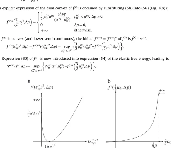
pÞ2: ð58Þ

An explicit expression of the dual convex of f(r)_{is obtained by substituting (58) into (56) (Fig.1(b)):}

fðrÞn 3 2

m

ðrÞ 0,

D

p ! " ¼ 3 2

m

ðrÞ 0

m

ðrÞ ð

D

pÞ2 ð

m

ðrÞ_'

m

ðrÞ 0Þ

m

ðrÞ 0 o

m

ðrÞ,

D

pZ0, 0,

D

p ¼ 0, þ1 otherwise: 8 > > > > < > > > > : ð59Þ

As fðrÞ_{is convex (and lower semi-continuous), the bidual f}ðrÞnn

& ðfðrÞn Þnof f(r)_{is f}(r)_itself: fðrÞ_ðð

_e

tr eqÞ2,

D

pÞ ¼ fðrÞ nn ðð

e

treqÞ2,

D

pÞ ¼ sup mðrÞ 0rmðrÞ 3 2

m

ðrÞ 0ð

e

treqÞ2'fðrÞ n 3 2

m

ðrÞ 0,

D

p ! " % & : ð60Þ

Expression (60) of fðrÞ_{is now introduced into expression (54) of the elastic free energy, leading to}

C

eðrÞ_ð

_e

tr_,

_D

_{pÞ ¼ sup} mðrÞ 0rmðrÞ WðrÞ 0 ð

e

tr,

m

ðrÞ0 Þ'fðrÞ n 3 2

m

ðrÞ 0,

D

p ! " % & , ð61Þ

Fig. 1. The function f ððetr

eqÞ2,DpÞ (a) and its convex dual by the Legendre transform, fnð23m0,DpÞ (b).Dpacts as a parameter, which is taken positive in the

where WðrÞ

0 is similar in form to the elastic energy of a linear, isotropic material:

WðrÞ 0 ð

e

tr,

m

ðrÞ0Þ ¼92

k

ðrÞð

e

trmÞ2þ32

m

ðrÞ0 ð

e

treqÞ2¼12

e

tr: CðrÞ0 :

e

tr¼12ð

e

'

e

pnÞ : CðrÞ0 : ð

e

'

e

pnÞ, ð62Þ with CðrÞ 0 given by CðrÞ 0 ¼ 3

k

ðrÞI vol þ2

m

ðrÞ0I dev : ð63Þ

Therefore, the dual variable

m

ðrÞ

0 introduced by the Legendre transform plays the role of a shear modulus in a fictitious

linear elastic material with potential (62). Accordingly, it should be positive everywhere. It will be shown that it is indeed the case according to the model proposed in the next section. Note that

m

ðrÞ

0 fluctuates within phase r, according to its

expression (57). On the other hand, the plastic strain

e

pn plays the role of an eigenstrain field applied to the linear

comparison material.

The linearization suggested by the variational procedure can be interpreted as follows. Using expression (61) for the elastic part of the free energy, the local stress in the composite is given by

r

¼@

C

eðrÞ @

e

tr : @

e

tr @

e

e ¼ C ðrÞ 0 :

e

tr: ð64Þ

Thus, the comparison moduli CðrÞ

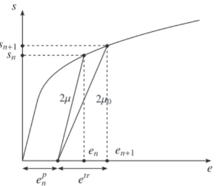
0 play the role of secant moduli in the stress–trial strain relation (Fig.2). The linearization

technique involved in the present approach can therefore be referred to as a trial, secant method.

Remark 3. Interestingly, the comparison shear modulus

m

0 (57) coincides with coefficient k2in the following spectral

decomposition of the algorithmic tangent operator of J2plasticity:

Calg

¼ 3k1Cð1Þþ2k2Cð2Þþ2k3Cð3Þ, ð65Þ

where tensors CðiÞ _{are given by}

Cð1Þ_{¼ I}vol_{, C}ð3Þ_¼2

3N % N, Cð2Þ¼ Idev'23N % N, ð66Þ

and satisfy: CðiÞ_{: C}ðjÞ_¼

_d

ijCðiÞ (no sum over i). The decomposition (65) was introduced by Ponte Castan˜eda (1996)for

tangent operators in nonlinear elasticity. When applied to the algorithmic tangent operator of J2 elasto-plasticity, the

coefficients kiread (Doghri and Ouaar, 2003, recall that

s

treq¼ 3

me

treqÞ

k1¼

k

, k2¼

m

1'3

m

D

p

s

tr eq ! , k3¼

m

1' 3

m

3

m

þR0_ðpÞ ! " : ð67Þ 4.2. Overall potential

We now use the linearization technique presented in the previous section to express the overall potential of the composite in terms of the effective potential of a LCC. Substituting expression (61) together with (62) into that of the effective potential (50) leads to

W_Dð

e

Þ ¼ inf e2KðeÞ Dinfp Z 0_0osup_mðsÞ 0rmðsÞ Xn r ¼ 1

w

ðrÞ_{ðxÞ W}ðrÞ 0 ð

e

'

e

pn,

m

ðrÞ0Þ'fðrÞ n 3 2

m

ðrÞ 0 ,

D

p ! " þ

c

pðrÞðpnþ

D

pÞ'

c

ðrÞnðxÞþ

D

t

f

ðrÞ

D

p

D

t ! " ! " ( ) * + , ð68Þ in which the condition

D

pZ0 follows from the specific form (41) of the dissipation function. The expression between curly brackets is convex in

e

(under the ansatz that

m

ðrÞ

0 is positive) and concave w.r.t.

m

ðrÞ0. According to the saddle-point theorem

(Rockafellar, 1970), the order of the infimum w.r.t.

e

and supremum w.r.t.

m

ðrÞ

0 can be interchanged, and an alternative

Fig. 2. The proposed variational formulation can be interpreted as a secant method based on the elastic trial strain:etr

representation is obtained: W_Dð

e

Þ ¼ inf Dp Z 0_0osup_mðsÞ 0rmðsÞ W0ð

e

,

m

ðsÞ0Þþ Xn r ¼ 1

w

ðrÞ_{ðxÞ 'f}ðrÞn 3 2

m

ðrÞ 0,

D

p ! " þ

c

pðrÞ_ðp nþ

D

pÞ'

c

ðrÞnðxÞþ

D

t

f

ðrÞ

D

p

D

t ! " ! " * + ( ) , ð69Þ where W0is the effective potential of a LCC characterized by phase potentials W0ðrÞ:

W0ð

e

,

m

ðsÞ0Þ ¼ inf_e 2KðeÞ Xn r ¼ 1

w

ðrÞ_ðxÞWðrÞ 0 ð

e

'

e

pn,

m

ðrÞ0Þ * + : ð70Þ

The expression between curly brackets in (69) is not convex w.r.t.

D

p, so that the order of the infimum and supremum operations may not be inverted. Accounting for the stationarity w.r.t. the fields

m

ðrÞ

0 and

D

p, the overall stress of the

composite is given by

r

¼@WD @

e

ð

e

Þ ¼ @W0 @

e

ð

e

,

m

ðsÞ 0Þ: ð71Þ

The formulation (69) of the homogenization problem, supplemented by the local flow rule (21), is completely equivalent to the original one (50), and is therefore as complicated to solve. However, it involves the effective energy of a LCC, which constitutes the first step towards the derivation of estimates.

4.3. Approximation by piecewise uniform shear moduli

A straightforward (and probably unavoidable) approximation to formulation (69) consists in considering piecewise uniform shear moduli within the LCC:

m

0ðxÞ ¼ XN r ¼ 1

w

ðrÞ_ðxÞ

_m

ðrÞ 0, ð72Þ where

m

ðrÞ

0 is now uniform in phase r. This corresponds to a restriction of the solutions space in the variational problem

(69). In (72), it is assumed that the spatial distribution of the phases in the LCC coincides with the one in the actual composite.2

Approximation (72) also implies piecewise uniformity of the optimal field

D

pðxÞ, solution of the variational problem (69). Indeed, consider the composite in a strain- and stress-free configuration at t¼t0, so that pnis initially piecewise

uniform (and zero). As all terms involving p and/or

D

pin the functional between curly brackets in Eq. (69) are piecewise uniform, it follows that

D

pðxÞ solution of the infimum problem at t1 is also piecewise uniform. Applying the same

reasoning at each subsequent time step, the fields

D

pðxÞ, as well as pðxÞ at any time tn þ 1are necessarily piecewise uniform.

5. An estimate based on uniform eigenstrain

The piecewise uniformity of the shear moduli and the internal variable p (as a consequence) dramatically reduces the difficulty of problem (69). However, the eigenstrain field

e

pnin (70) fluctuates within each plastic phase, preventing a direct

application of linear estimates for thermoelastic composites. Therefore, an additional approximation is required, which might consist in considering a uniform, reference plastic strain at tnfor each phase in expression (70). A rather intuitive

choice is to set the reference plastic strain equal to the average of the plastic strain in the phase. Unfortunately, results obtained so far under this assumption turned out to be inconsistent in most examples of particulate composites reinforced by elastic inclusions (Brassart, 2011).

The estimate proposed and validated in the sequel is based on a different, and yet simpler modeling assumption of a uniformreference plastic strain for the whole composite. The effective potential (70) of the LCC is then approximated as

W0ð

e

,

m

ðsÞ0Þ , ~W0ð

e

,

m

ðsÞ0Þ ¼ inf_e 2KðeÞ Xn r ¼ 1

w

ðrÞ_ðxÞWðrÞ 0 ð

e

'^

e

p n,

m

ðrÞ0Þ * + , ð73Þ

where ^

e

pnis the reference plastic strain, given by

^

e

pn& /

e

pnS: ð74Þ

Then, the effective potential of the LCC is simply given by ~

W0ð

e

,

m

ðsÞ0Þ ¼12ð

e

'/

e

pnSÞ : C0: ð

e

'/

e

pnSÞ, ð75Þ

whereC0is the overall elastic stiffness of the LCC, to be computed from any linear scheme suited for the microstructure

under consideration.

2_{This prescription is not absolutely necessary, nor necessarily optimal, as noted bySuquet (1993). However, the question of considering a LCC with a}

The proposed simplified model considers the LCC to be subjected to a uniform pre-deformation corresponding to the average plastic deformation at the previous time step. With such simplification, inter-phase (as well as intra-phase) plastic strain heterogeneities are overlooked when solving the LCC problem. Note however that the actual plastic strain field is not supposed to be uniform: the uniform reference plastic strain is used for the localization step only. Updates for the per-phase averages of the plastic strain will be described later. Despite the apparent crudeness of prescription (74), valuable predictions are obtained when the model is applied to two-phase particulate composites, as shown inSection 6. Remark 4. Adopting the following change of variable:

e

0_{ðxÞ &}

_e

_ðxÞ'^

_e

p

n, where

e

ðxÞ is the strain field solution of problem

(73), the latter is equivalently reexpressed as ~ W0ð

e

,

m

ðsÞ0Þ ¼ inf e0_2KðetrÞ XN r ¼ 1

w

ðrÞ_ðxÞWðrÞ 0 ð

e

0,

m

ðrÞ0 Þ * + , ð76Þ

where

e

tr&

e

'/

e

pnS. Note that the field

e

0is compatible.

According to (71), the macroscopic stress in the nonlinear composite is given by the macroscopic stress in the LCC:

r

¼ C0: ð

e

'/

e

pnSÞ: ð77Þ

Relation (77) also implies that the volume average of the stress in the nonlinear composite and in the LCC coincide. Therefore, it seems natural to approximate per-phase averages of the stress in the nonlinear composite by corresponding ones in the LCC:

/

r

Sr¼ /

r

0Sr, ð78Þ

where

r

0_{denotes the stress field in the LCC with uniform eigenstrain. We will further assume that moments of the trial}

strain field in the nonlinear composite are approximated by corresponding moments of the field

e

0 _{computed in the LCC:}

/

e

tr_S

r¼ /

e

0Sr, /ð

e

treqÞ2Sr¼ /ð

e

0eqÞ2Sr: ð79Þ

5.1. Optimization w.r.t.

m

ðrÞ

0 and

D

pðrÞ

Adopting expression (76) for the effective potential of the LCC, we now address the optimization w.r.t.

m

ðrÞ

0 and

D

pðrÞin

(69). The stationarity condition w.r.t.

m

ðrÞ 0 writes @ ~W0 @

m

ðrÞ₀ 'cr @fnðrÞ @

m

ðrÞ₀

m

ðrÞ 0,

D

pðrÞ ( ) * + r ¼ 0: ð80Þ

A classical result in the homogenization of linear composites indicates that the first term in the left-hand side member can be rewritten in terms of the second moment of the strain field in the LCC as (Bobeth and Diener, 1986;Kreher, 1990;Ponte Castan˜eda and Suquet, 1998)

@ ~W0 @

m

ðrÞ₀ ¼ 3 2cr/ð

e

0eqÞ2Sr¼ 3 2cr/ð

e

tr eqÞ2Sr, ð81Þ

where the last equality follows from assumption (79). On the other hand, the derivative of fðrÞ

n w.r.t.

m

ðrÞ₀ gives @fnðrÞ @

m

ðrÞ₀ ð

m

ðrÞ 0,

D

pðrÞÞ ¼ 3 2

m

ðrÞ

_D

_pðrÞ

m

ðrÞ_'

m

ðrÞ 0 !2 : ð82Þ

Combining the last three equations and accounting for the homogeneity of

D

pðrÞ_{, one obtains an explicit expression of the}

effective shear moduli which is similar in form to (57):

m

ðrÞ 0 ¼

m

ðrÞ 1'

D

pðrÞ ffiffiffiffiffiffiffiffiffiffiffiffiffiffiffiffiffiffiffiffiffi /ð

e

tr eqÞ2Sr q 0 B @ 1 C A: ð83Þ

Taking the stationarity w.r.t.

m

ðrÞ

0 into account, the minimization w.r.t.

D

pðrÞyields the following condition in phase r:

'3

m

ðrÞ

m

ðrÞ0

m

ðrÞ_'

_m

ðrÞ 0

D

pðrÞ_þRðrÞ_ðpðrÞ n þ

D

pðrÞÞþ @

f

ðrÞ @ _p

D

pðrÞ

D

t ! " ¼ 0, ð84Þ

or, making use of (83): '3

m

ðrÞ ffiffiffiffiffiffiffiffiffiffiffiffiffiffiffiffiffiffiffiffiffi_/ð

_e

tr eqÞ2Sr q þ3

m

ðrÞ

_D

_pðrÞ_þRðrÞ_ðpðrÞ n þ

D

pðrÞÞþ @

f

ðrÞ @ _p

D

pðrÞ

D

t ! " ¼ 0: ð85Þ

Recalling Eq. (33), Eq. (85) can be interpreted as a homogenized radial return equation for phase r. A positive

D

pðrÞ_solution

left-hand side of (85). The unique yield criterion for phase r reads '3

m

ðrÞ ffiffiffiffiffiffiffiffiffiffiffiffiffiffiffiffiffiffiffiffiffi_/ð

_e

tr eqÞ2Sr q þRðrÞ_ðpðrÞ n Þþ

s

ðrÞY o0: ð86Þ

In the yield criterion (86) the second moment/ð

e

tr

eqÞ2Sris computed on the LCC characterized by the elastic shear moduli

m

ðrÞ_{. Indeed,}

_m

ðrÞ

0 -

m

ðrÞas

D

pðrÞ-0, according to expression (83). If the yield criterion (86) is not satisfied, the increment is

elastic in phase r, and the minimum is achieved for

D

pðrÞ_{¼ 0. Otherwise, the radial return condition (85) takes the familiar}

form (35): '3

m

ðrÞ ffiffiffiffiffiffiffiffiffiffiffiffiffiffiffiffiffiffiffiffiffi /ð

e

tr eqÞ2Sr q þ3

m

ðrÞ

D

pðrÞ_þRðrÞ_ðpðrÞ n þ

D

pðrÞÞþ

s

ðrÞY ¼ 0: ð87Þ

Since Eq. (87) may be rewritten as ffiffiffiffiffiffiffiffiffiffiffiffiffiffiffiffiffiffiffiffiffi /ð

e

tr eqÞ2Sr q ¼

D

pðrÞ_þ 1 3

m

ðrÞðRðrÞðpðrÞn þ

D

pðrÞÞþ

s

ðrÞYÞ, ð88Þ

the second term of the right hand side is always positive. Hence, ffiffiffiffiffiffiffiffiffiffiffiffiffiffiffiffiffiffiffiffiffi/ð

e

tr eqÞ2Sr

q

4

D

pðrÞ _and

_m

ðrÞ

0 is always positive, as

announced.

5.2. Homogenized flow rule

The proposed estimate of the composite mechanical response also requires computation of the phase average of the plastic strain (or plastic strain increment) at each time step:

/

D

e

p_{S ¼} XN r ¼ 1 cr/

D

e

pSr¼ XN r ¼ 1 cr

D

pðrÞ e tr

e

tr eq * + r : ð89Þ

The average plastic strain update is computed by making use of the following observations. On the one hand, the phase average of the stress is given by

/

r

Sr¼ CeðrÞ:/

e

tr'

D

e

pSr¼ CeðrÞ:/

e

trSr'2

m

ðrÞ/

D

e

pSr: ð90Þ

On the other hand, according to (78), we also have /

r

Sr¼ /

r

0Sr¼ CðrÞ0 :/

e

0Sr¼ CeðrÞ:/

e

0Sr'2

m

ðrÞ

D

pðrÞ /e0_S r ffiffiffiffiffiffiffiffiffiffiffiffiffiffiffiffiffiffiffiffiffi /ð

e

0 eqÞ2Sr q : ð91Þ

The last equality is obtained using expression (83) of the shear modulus

m

ðrÞ

0 . Making use of assumption (79), a direct

comparison of the last two expressions yields /

D

e

p_S r¼

D

pðrÞ etr

e

tr eq * + r ¼

D

pðrÞ /etrSr ffiffiffiffiffiffiffiffiffiffiffiffiffiffiffiffiffiffiffiffiffi /ð

e

tr eqÞ2Sr q , ð92Þ

which defines an effective flow direction NðrÞ_{for phase r:}

NðrÞ_{& ffiffiffiffiffiffiffiffiffiffiffiffiffiffiffiffiffiffiffiffiffi}/etrSr

/ð

e

tr eqÞ2Sr

q : ð93Þ

Eq. (92) can be viewed as a homogenized plastic flow rule for the average plastic strain. Remark 5. In general, NðrÞ_{: N}ðrÞ_{a3=2. Instead:}

NðrÞ_{: N}ðrÞ_¼3 2 ð/

e

tr_S rÞ2eq /ð

e

tr eqÞ2Sr , ð94Þ

where the second-order moment of

e

tr_{is necessarily greater than the first-order moment, except in very specific situations}

where fields are homogeneous in each phase. 5.3. Summary of the homogenization procedure

Taking advantage of formulation (76) for the effective behavior of the LCC, algorithmic implementation is rather straightforward. We consider a composite in a strain- and stress-free configuration at t¼t0. On a time interval ½tn,tn þ 1), history

variables at tnare given for each phase r:/

e

pnSrand/pnSr. Given

e

, the macroscopic strain at tn þ 1, the problem is to compute

the macroscopic stress

r

. In the proposed numerical procedure, we iterate on the value of the reference shear moduli

m

ðrÞ 0.

- Elastic predictor step. Taking

m

ðrÞ0 ¼

m

ðrÞ:

1. Compute the effective stiffness C0 according to the chosen homogenization scheme for a linear elastic composite.

Next, compute/ð

e

tr

2. Evaluate the yield criterion (86) in each phase: kðrÞ_{ðrÞ & '3}

_m

ðrÞ ffiffiffiffiffiffiffiffiffiffiffiffiffiffiffiffiffiffiffiffiffi_/ð

_e

tr eqÞ2Sr q þRðrÞ_ðpðrÞ n Þþ

s

ðrÞY:

3. If kðrÞ_{Z0: the increment is elastic in phase r, and}

_m

ðrÞ

0 ¼

m

ðrÞand

D

pðrÞ¼ 0.

4. Otherwise,

m

ðrÞ

0 is smaller than

m

ðrÞand it must be found iteratively.

- Plastic correction step. Iteration (i) (upper index (i) omitted for simplicity). Compute the effective stiffness C0according

to the chosen homogenization scheme for a linear elastic composite. For each phase r in which plastic yielding occurs: 1. Compute/ð

e

tr

eqÞ2Sr according to Eq. (81).

2. Compute

D

pðrÞ_{according to Eq. (83):}

D

pðrÞ_¼

m

ðrÞ'

m

ðrÞ 0

m

ðrÞ ffiffiffiffiffiffiffiffiffiffiffiffiffiffiffiffiffiffiffiffiffi /ð

e

tr eqÞ2Sr q :

3. Compute the residual (radial return Eq. (87)): FðrÞ_{& '3}

_m

ðrÞ ffiffiffiffiffiffiffiffiffiffiffiffiffiffiffiffiffiffiffiffiffi_/ð

_e

tr eqÞ2Sr q þ3

m

ðrÞ

D

pðrÞ_þRðrÞ_ðpðrÞ n þ

D

pðrÞÞþ

s

ðrÞY : Iterate on

m

ðrÞ

0 until the absolute value of the residual in each phase becomes lower than a given tolerance.

- After convergence. Compute the increment of average plastic strain: /

D

e

p_S r¼

D

pðrÞ /e tr_S r ffiffiffiffiffiffiffiffiffiffiffiffiffiffiffiffiffiffiffiffiffi /ð

e

tr eqÞ2Sr q ,

and update the internal variables: /

e

p_S

r¼ /

e

pnSrþ/

D

e

pSr,

pðrÞ_{¼ p}ðrÞ n þ

D

pðrÞ:

Finally, the macroscopic stress is obtained from the effective stiffness of the LCC as

r

¼ C0: ð

e

'/

e

pnSÞ ¼ /

r

S:

In cases where an expression for the effective stiffness C0is available in closed form, the procedure is implemented using

the Newton–Raphson method. In the examples of the next section, three iterations are typically sufficient to reach convergence.

6. Application to two particle-reinforced composites

In this section we compare the predictions of the simplified model proposed inSection 5to reference results obtained from full-field finite element (FE) simulations for several two-phase composites. We consider composites made of a square array of spherical inclusions, which are frequently approximated by axisymmetric unit cells (Fig.3(a)) allowing full-field computations at low cost. The geometry is meshed using the GMSH software (Geuzaine and Remacle, 2009), and a typical mesh comprises approximately 1000 elements and 2700 nodes (Fig. 3(b)). A convergence study was successfully conducted by comparing the predictions to those obtained with finer meshes (about 2500 elements). FE computations are performed usingABAQUS 6.9 (2009)using quadratic CAX6 and CAX8 elements. Reference, FE predictions are labeled ‘‘FE’’ in the figures.

Regarding the simplified model, two approaches have been pursued to solve the localization problem over the LCC. On the one hand, the LCC is homogenized ‘‘exactly’’ using the FE method. In this case, first- and second-order moments of stress and strain fields involved in the procedure are computed from direct volume averaging of the local fields in the LCC.

Fig. 3. (a) Reference predictions for composites with periodic microstructure are obtained considering cylindrical unit cells. (b) FE computations are performed using axisymmetric elements.

In this way, the linearization procedure, together with the other approximation introduced inSection 5, are assessed while avoiding additional errors related to the use of an approximate linear homogenization scheme. This methodology was already used in order to evaluate the capabilities of linearization methods byRekik et al. (2007)andLahellec and Suquet (2007a). Corresponding results are labeled ‘‘VARþFE’’ in the figures.

Alternatively, (hopefully) reliable estimates of the effective response of inclusion-reinforced linear elastic composites are provided by Hashin–Shtrikman (HS) lower bound (Hashin and Shtrikman, 1963;Willis, 1977). An advantage of the HS bounds is the relative simplicity of implementation: an expression of the effective stiffness of the LCC is then available in closed-form. The predictions of the variational method combined with the HS lower bound are labeled ‘‘VARþHS-’’ in the figures.

The composites are subjected to uniaxial tension in the z-direction. The boundary conditions applied to the unit cell are the following:

u3ðr,z ¼ H=2Þ ¼ u3, 0oroR,

u3ðr,z ¼ 0Þ ¼ 0, 0or oR,

u1ðr ¼ 0,zÞ ¼ 0, 0ozoH=2,

u1ðr ¼ R,zÞ ¼ u1, 0ozoH=2,

with H¼2R. The displacement u3is prescribed, while u1is a priori unknown as the r¼R boundary is traction-free. Loading

involves 50 time increments unless otherwise indicated. 6.1. Elastic inclusions, elasto-plastic matrix

The material under consideration is a metal matrix composite (MMC) with the following properties:

-

Inclusions (phase 1): E¼400 GPa,

n

¼ 0:2.

-

Matrix (phase 2): E¼75 GPa,

n

¼ 0:3,

s

Y¼ 75 MPa, RðpÞ ¼ hpn, h¼400 MPa, n¼0.4 or n¼0.05.

Two volume fractions of inclusions are considered: c1¼0.15 and c1¼0.30. MMC’s with similar material properties were

previously considered by several authors aiming to assess homogenization models (Segurado et al., 2002; Michel and Suquet, 2003; Doghri and Ouaar, 2003; Gonza´lez et al., 2004; Chaboche et al., 2005; Pierard et al., 2007) so that the predictive capabilities of the present approach can easily be evaluated w.r.t. those schemes.

The effective response for both hardening exponents and volume fractions is presented inFig. 4. The VARþFE model gives satisfying predictions for both volume fractions in the case n¼0.4, while it overestimates the reference response when n¼0.05. In the latter case, better predictions are obtained using HS lower bound to homogenize the LCC (VARþHS-model), due to the compensation of errors between the underestimation brought by the HS lower bound and the overestimation due to the present choice of LCC. On the other hand, the prediction of the VARþHS-model are too soft in the case c1¼0.30 and n¼0.4.

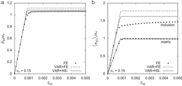
The accuracy of the model regarding the phase response is assessed in Fig. 5taking c1¼0.15. For both hardening

exponents, the proposed estimate correctly predicts the matrix response, even without the additional underestimation brought by the HS model. The evolution of the accumulated plastic strain in the matrix is also very well captured by the homogenization models (not shown). The method is less accurate regarding the inclusion response. There is a large discrepancy between VARþFE and VARþHS-results observed in the inclusions, while they are remarkably close in the matrix.

Previous examples showed that the model is less accurate when the matrix presents weak hardening. A limit case is obtained considering a perfectly plastic matrix: R(p)¼0 (other material properties left unchanged). As expected from previous observations, the VARþFE model overestimates the effective response (Fig. 6(a)), due to an unsuccessful prediction of the inclusion response (Fig. 6(b)). Predictions are more accurate using HS lower bound to homogenize the LCC.

Convergence of the model is analyzed inFig. 7for c1¼0.15 and n¼0.4, by successively considering 20, 50 and 100

increments to achieve the total elongation. It has been checked against results obtained using a very large number of increments (up to 10 000) that the curve with 100 increments can be considered as a converged result. The scatter between the stress–strain curves presented in the figure is very low, as required. Obviously, sufficiently small loading steps are needed to capture the elastic–plastic transition accurately. Similar conclusions hold for n¼0.05 and the case of a perfectly plastic matrix.

The variational procedure is able to simulate non-monotonic loadings. Examples of uniaxial tension/compression tests for c1¼0.15 and c1¼0.30 are presented inFig. 8, taking n¼0.4. The figure shows comparable accuracy of the proposed

models in tension and compression. For c1¼0.30, the full-field simulation demonstrates a Baushinger effect (early and

progressive plastification in the unloading branches of the cycle). Such effect is related to the heterogeneity of the plastic strain field which developed during the initial step of uniaxial tension. The proposed model predicts a sharp elastic–plastic

0 1 2 3 4 5 6 7 8 0 0.01 0.02 0.03 0.04 0.05 ¯σ33 /σY ¯ε33 n = 0.05 n = 0.4 c1 = 0.15 FE VAR+FE VAR+HS-0 2 4 6 8 10 0 0.01 0.02 0.03 0.04 0.05 ¯σ33 /σY ¯ε33 n = 0.05 n = 0.4 c1 = 0.30 FE VAR+FE

VAR+HS-Fig. 4. Macroscopic response of a periodic composite with an elasto-plastic matrix and elastic inclusions for two volume fractions of inclusions: c1¼0.15

(a) and c1¼0.30 (b) and two different matrix hardening exponents: n¼0.05 and n¼0.4.

0 1 2 3 4 5 6 0 0.01 0.02 0.03 0.04 0.05 ¯ε33 ¯ε33 inclusion matrix c1 = 0.15 n = 0.4 FE VAR+FE VAR+HS-0 2 4 6 8 10 12 0 0.01 0.02 0.03 0.04 0.05 σ33 r /σY σ33 r /σY inclusion matrix c1 = 0.15 n = 0.05 FE VAR+FE

VAR+HS-Fig. 5. Phase response of a periodic composite with an elasto-plastic matrix and elastic inclusions (c1¼ 0:15Þ for two different matrix hardening

transition in compression, as the homogenized yield criterion (86) for the matrix phase accounts for isotropic hardening only. Nevertheless, the stress level after the effective elastic–plastic transition is correctly predicted by the VARþFE model. 6.2. Elasto-plastic inclusions, elasto-plastic matrix

We continue with a composite made of two elasto-plastic phases:

-

Inclusions (phase 1): E¼400 GPa,

n

¼ 0:2,

s

Y¼ 75 MPa, Rð1ÞðpÞ ¼ hð1Þpnð1Þ, hð1Þ¼ 1 GPa, nð1Þ¼ 0:4 or nð1Þ¼ 0:05.

-

Matrix (phase 2): E¼75 GPa,

n

¼ 0:3,

s

Y¼ 75 MPa, Rð2ÞðpÞ ¼ hð2Þpnð2Þ, hð2Þ¼ 400 MPa, nð2Þ¼ 0:4 or nð2Þ¼ 0:05.

The volume fraction of inclusions is c1¼0.15.

The effective response of the composite is presented inFig. 9for all combinations of inclusion and matrix hardening exponents. The responses for nð1Þ_{¼ 0:05 inFig. 9(a) are very close to those presented inFig. 4(a) for composites reinforced}

by elastic inclusions. Indeed, it can be checked that plastic deformations in the inclusions are negligible (although non-zero). On the contrary, when nð1Þ_{¼ 0:4 (Fig.9(b)), plastic deformations are important in both phases. Interestingly, the}

VARþFE and VARþHS-models predict almost identical effective response, whereas this is not necessarily true at the phase level. 0 0.2 0.4 0.6 0.8 1 1.2 ¯σ33 /σY c1 = 0.15 FE VAR+FE VAR+HS-0 0.5 1 1.5 2 0 0.001 0.002 0.003 0.004 0.005 0 0.001 0.002 0.003 0.004 0.005 σ33 r /σY ¯ε33 ¯ε33 inclusion matrix c1 = 0.15 FE VAR+FE

VAR+HS-Fig. 6. Macroscopic (a) and phase (b) response of a periodic composite with a perfectly plastic matrix (RðpÞ ¼ 0) and elastic inclusions (c1¼0.15).

0 0.5 1 1.5 2 2.5 3 0 0.01 0.02 0.03 0.04 0.05 ¯σ33 /σY ¯ε33 c1 = 0.15 n = 0.4 VAR+HS-, ∆¯ε33 = 2.5 × 10−3 ∆¯ε33 = 1 × 10−3 ∆¯ε33 = 5 × 10−4

Fig. 7. Macroscopic response of a periodic composite with an elasto-plastic matrix (n¼0.4) and elastic inclusions (c1¼ 0:15Þ as predicted by the

-6 -4 -2 0 2 4 6 ¯σ33 /σY ¯ε33 c1 = 0.15 n = 0.4 FE VAR+FE VAR+HS--8 -6 -4 -2 0 2 4 6 8 -0.06 -0.04 -0.02 0 0.02 0.04 0.06 -0.06 -0.04 -0.02 0 0.02 0.04 0.06 ¯σ33 /σY ¯ε33 c1 = 0.30 n = 0.4 FE VAR+FE

VAR+HS-Fig. 8. Macroscopic response of a periodic composite with an elasto-plastic matrix (n¼0.4) and elastic inclusions, for c1¼0.15 (a) and c1¼0.30 (b).

0 1 2 3 4 5 6 7 8 0 0.01 0.02 0.03 0.04 0.05 ¯σ33 /σY ¯ε33 n(2) _{= 0.05} n(2) _{= 0.4} c1 = 0.15 n(1) _{= 0.05} FE VAR+FE VAR+HS-0 1 2 3 4 5 6 7 8 0 0.01 0.02 0.03 0.04 0.05 ¯σ33 /σY ¯ε33 n(2) _{= 0.05} n(2) _{= 0.4} c1 = 0.15 n(1) _{= 0.4} FE VAR+FE

6.3. Perfectly plastic inclusions and matrix

Finally, we consider the case of two perfectly plastic phases: Rð1Þ_{ðpÞ ¼ R}ð2Þ_{ðpÞ ¼ 0 with identical yield stresses but distinct}

elastic properties, identical to those considered before. The overall yield stress of the composite is obviously

s

Y¼

s

ð1ÞY ¼

s

ð2ÞY , and the heterogeneous elastic properties should affect only the macroscopic yield strain. Unfortunately,

the variational procedure fails to predict the exact overall yield stress (Fig. 10(a)). Worse: a strong dependence on the number of loadsteps is observed, with the overall yield stress decreasing when the load increment is reduced (Fig.10(b)). A look at the phase response (not shown) shows that the matrix stress never reaches the yield point, while the inclusion plastic strain is overestimated.

These results illustrate the limits of the proposed model in which plastic strain incompatibilities are neglected for the localization step. In the present example, inclusions are stiffer than the matrix and reach their yield point first. After several load increments, the average plastic strain update is observed to tend towards the macroscopic strain increment:

/

D

e

p_{S ¼ c}

1/

D

e

pS1-

D

e

: ð95Þ

As the (uniform) eigenstrain increases at the same rate as the macroscopic strain, moments of the trial strain in the phases (estimated by corresponding moments of the field

e

0_¼

_e

_'/

_e

p_{nS in the LCC, see relations (79)) reach a constant value, so as}

D

pðrÞ_and

_m

ðrÞ

0 . Consequently, when this ‘‘regime’’ stage is reached, the phase and macroscopic stress tend to a constant

value. Such behavior can be intuitively understood comparing (95) with a similar relation in homogeneous perfect plasticity, where

_

e

p_{-_}

_e

_{or, incrementally}

_D

_e

p_-

_D

_e

_{, ð96Þ}

from which it also follows that

D

e

tr_{-0. Only one load step in homogeneous, perfect plasticity suffices to reach the regime.}

In the composite, this number is higher (here, about 8), and does not seem to depend on the level of macroscopic strain. Consequently, the regime is reached at lower macroscopic strain when the load increment is reduced, causing the load step sensitivity shown inFig. 10(b).

7. Concluding remarks

Section 4presented an original equivalent formulation of the homogenization problem involving the potential of a thermoelastic composite in which the plastic strain field at the previous time step plays the role of an eigenstrain field. In

Section 5, the composite mechanical response was estimated based on the following approximations: (i) piecewise uniform comparison moduli (and accumulated plastic strain as a consequence) and (ii) uniform reference plastic strain for tnfor the whole composite. The first approximation is commonly adopted in variational procedures (like the variational

procedure of Ponte Castan˜eda, 1991) and seems unavoidable. The second one amounts to neglect both intra- and inter-phase plastic strain incompatibilities when solving the localization problem on the LCC. Previous plastic strain is accounted for on average only. Despite this rough approximation, the estimate provides fairly good predictions in most examples tested so far in the context of two-phase particulate composites. A notable exception is the case of a composite

0 0.2 0.4 0.6 0.8 1 1.2 ¯σ33 /σY ¯ε33 c1 = 0.15 FE VAR+FE VAR+HS-0 0.2 0.4 0.6 0.8 1 1.2 0 0.001 0.002 0.003 0.004 0.005 0 0.001 0.002 0.003 0.004 0.005 ¯σ33 /σY ¯ε33 ∆¯ε33 = 1 × 10−4 ∆¯ε33 = 5 × 10−5 ∆¯ε33 = 5 × 10−6 c1 = 0.15 _VAR+HS-VAR+FE

Fig. 10. (a) Macroscopic response of a periodic composite with a perfectly plastic matrix and perfectly plastic inclusions (c1¼0.15). Both phases have the

same yield stress. (b) The convergence of the VARþFE and VARþHS-models is assessed by considering successively 50, 100 and 1000 strain increments to reach the final elongation.

with two perfectly plastic phases having the same yield stress (Section6.3). In this case, neglecting inter-phase plastic incompatibilities leads to inconsistent results.

Important aspects of the proposed method are summarized:

-

The model is designed for true elasto-plasticity, and does not require the approximation of visco-plasticity or perfect plasticity. One explicitly accounts for the existence of an elasticity domain, nonlinear hardening, and the hereditary behavior. In particular, arbitrary loading paths are handled.

-

The formulation suggests an original localization rule for elasto-plastic composites based on ‘‘trial secant’’ operators computed for the second moments of the trial strain field. These operators are softer than the corresponding elastic ones.

-

The algorithmic structure of the incremental equations of elasto-plasticity is preserved in the homogenization scheme. The model yields a homogenized yield criterion for each elasto-plastic phase, and a homogenized radial return equation for the internal variable. Both the homogenized yield criterion and the return mapping equation are based on the second-order moment of the trial strain field as a result from the variational procedure. A homogenized flow rule for per-phase averages of the plastic strain was also derived.

Future developments of the approach should focus on the account of inter-phase plastic strain incompatibilities in the localization problem. This can be achieved considering piecewise uniform reference plastic strain in the thermoelastic problem (70), instead of a uniform one. However, the definition of a proper uniform reference plastic strain for the phase is not straightforward (Lahellec and Suquet, 2007a;Brassart, 2011), and is left for future work.

Acknowledgments

L.B. and L.D. are mandated by the National Fund for Scientific Research (FNRS, Belgium). The authors thank the reviewer for a very constructive review which pointed out shortcomings in the initial manuscript, and N. Lahellec for helpful discussions.

Appendix A. Computation of the kinematic variable using Lagrange multipliers

The kinematic variable N must minimize the functional JD (23) under constraints (6). The corresponding Lagrangian

functional reads Lð

e

n þ 1,pn þ 1,N,

l

1,

l

2Þ ¼ 1 2 ð

e

tr n þ 1'

D

pNÞ : Ce: ð

e

trn þ 1'

D

pNÞþ

c

pðpn þ 1Þ'

c

nþ

D

t

f

D

p

D

t ! " þ

l

1trðNÞþ

l

2 N : N' 3 2 ! " : ð97Þ The kinematic variable N must satisfy the following condition:

@L

@Nð

e

n þ 1,pn þ 1,N,

l

1,

l

2Þ ¼ 0, ð98Þ

that is,

0 ¼ '

D

pCe: ð

e

tr

n þ 1'

D

pNÞþ

l

11þ2

l

2N ¼ '

D

pð

r

trn þ 1'

D

pðCe: NÞÞþ

l

11þ2

l

2N: ð99Þ

Additional hypotheses about the free-energy function are required in order to determine N. Here, isotropic elasticity is assumed, so that the elastic stiffness tensor may be decomposed into volumetric and deviatoric parts, see expression (32). In this case, condition (99) becomes

'

D

p

r

tr

n þ 1'2

m

D

pN

* +

þ

l

11þ2

l

2N ¼ 0: ð100Þ

The trace of the above expression is computed, leading to

l

1¼13

D

ptrð

r

trn þ 1Þ, ð101Þ

which, introduced in (100) yields '

D

pð

r

tr

n þ 1'13trð

r

trn þ 1ÞÞ1þ2

m

ð

D

pÞ2N þ2

l

2N ¼ 0, ð102Þ

which can be rewritten as '

D

pðstr

n þ 1Þ ¼ '2

m

ð

D

pÞ2N'2

l

2N: ð103Þ

This equation shows that the direction N is ‘‘aligned’’ with the tensor str

n þ 1. The normalizing condition in (6) finally gives

N ¼3₂ s tr n þ 1

s

tr eq,n þ 1 : ð104Þ