How to obtain a lattice basis from a discrete projected space

HAL Id: hal-00267542

https://hal.archives-ouvertes.fr/hal-00267542

Submitted on 27 Mar 2008

HAL is a multi-disciplinary open access

archive for the deposit and dissemination of

sci-entific research documents, whether they are

pub-lished or not. The documents may come from

teaching and research institutions in France or

abroad, or from public or private research centers.

L’archive ouverte pluridisciplinaire HAL, est

destinée au dépôt et à la diffusion de documents

scientifiques de niveau recherche, publiés ou non,

émanant des établissements d’enseignement et de

recherche français ou étrangers, des laboratoires

publics ou privés.

How to obtain a lattice basis from a discrete projected

space

Nicolas Normand, Myriam Servières, Jean-Pierre Guédon

To cite this version:

Nicolas Normand, Myriam Servières, Jean-Pierre Guédon. How to obtain a lattice basis from a discrete

projected space. Discrete Geometry for Computer Imagery, Apr 2005, Poitiers, France. pp.153-160,

�10.1007/b135490�. �hal-00267542�

How to obtain a lattice basis from a discrete projected space

Nicolas Normand

IRCCyN/IVC UMR CNRS 6597

Abstract. Euclidean spaces of dimension n are characterized in discrete spaces by the choice of

lat-tices. The goal of this paper is to provide a simple algorithm finding a lattice onto subspaces of lower dimensions onto which these discrete spaces are projected. This first obtained by depicting a tile in a space of dimension n – 1 when starting from an hypercubic grid in dimension n. Iterating this process across dimensions gives the final result.

@inproceedings{normand2005dgci,

Author = {Normand, Nicolas and Servi{\‘e}res, Myriam and Gu{\’e}don, JeanPierre}, Booktitle = {Discrete Geometry for Computer Imagery},

Date = {2005-04},

Doi = {10.1007/b135490},

Editor = {Andres, {\’E}ric and Damiand, Guillaume and Lienhardt, Pascal}, Isbn = {3-540-25513-3},

Month = apr, Pages = {153-160},

Publisher = {Springer Berlin / Heidelberg}, Series = {Lecture Notes in Computer Science},

Title = {How to obtain a lattice basis from a discrete projected space}, Volume = {3429},

Year = {2005}}

How to Obtain a Lattice Basis from a Discrete

Projected Space

Nicolas Normand, Myriam Servi`eres and JeanPierre Gu´edon

IRCCyN/IVC, ´Ecole polytechnique, University of Nantes Rue Christian Pauc, 44306 Nantes

Abstract. Euclidean spaces of dimension n are characterized in discrete spaces by the choice of lattices. The goal of this paper is to provide a simple algorithm finding a lattice onto subspaces of lower dimensions onto which these discrete spaces are projected. This first obtained by depicting a tile in a space of dimension n_{− 1 when starting from an} hypercubic grid in dimension n. Iterating this process across dimensions gives the final result.

1

Introduction

Regular lattices constitute the cornerstone for the building of discrete geometry tools and also for bases of classical continuous space of functions. Of course, these regular lattices can be defined without any outside reference. However, the definition of the resulting lattice is not obvious when a problem is designed in a discrete space and when it is mandatory to go back and forth from this first space to an other discrete space using a given discrete transform. When the same problem is entirely defined in a discrete manner, the lattice identification problem can become even harder. This paradigm was used to construct a cryp-tographic/signature scheme using the NTRU lattice [1].In this case, the lattice identification leads to an NP-problem.

Lattice identifications have also been investigated by Conway and Sloane for sphere packing which results are mainly employed for vector quantization in the multimedia coding area [2]. In Sect. 2, the starting point to review the literature will lie into the continuous/discrete correspondence firstly established by Shannon and generalized by Unser-Aldroubi. This work allows to start with a basis through a tensorial product, to sample the continuous space to give a lattice onto which a Riesz functional basis will be defined.

The aim of this paper is then to demonstrate how to obtain an unitary tile with a regular lattice on the projection hyperplane with discrete projection directions. This will be performed in a general manner in Sect. 3. The fact that we restrict the projection operator to discrete projection is based on the attempt to get a simple way to obtain a lattice onto the hyperplane. The difficulty is then to extract the lattice from regular projection grids, i.e. not to oversample the hyperplane grid with unused points nor to undersample a grid from which the lattice would not be obtained.

In other words, each point of the discrete projection plane must have a pre-decessor in the initial space and each point of the initial lattice is projected onto an existing point.

2

Related Work

Starting with the construction of orthonormal bases that give regular tiling leads to the Gram-Schmidt orthonormalisation procedure that can be found in almost any algebra textbook [3]. Because of the normalization, the resulting basis can be easily discretised and replicated to give a regular tiling.

Following this path (starting from the continuous point of view and discretiz-ing afterward) any n dimensional continuous space will give regular tildiscretiz-ing from this unconstrained orthonormal continuous grid. As a matter of fact, Unser and Aldroubi have generalized the Shannon-Whittaker-Kotelnikov Sampling Theo-rem starting with this n-dimensional orthogonal basis then lattice [4, 5]. The initial purpose of this theorem is to use other functional bases than the Riesz bases {(sinc (kx), k ∈ Z)}.

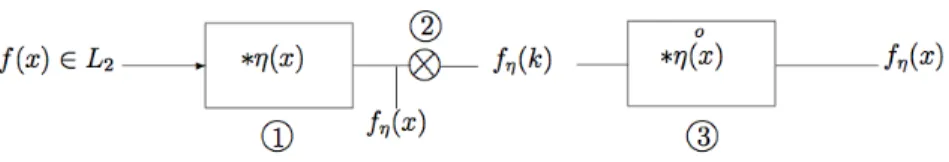
This theorem is described in Fig. 1

Fig. 1. Representation of the Unser-Aldroubi theorem

The first step corresponds to the orthogonal projection of the L2 function

f (x) onto a closed subspace of functions generated by a Riesz basis{η(kx), k ∈

Z}. In other words, these functions already need to be defined from a tiling (the first versions of the theorem corresponds to cardinal functions as the sinc for Shannon or cardinal splines for Unser-Aldroubi).

The second step also uses the same tiling but explicitly since it just picks up the values onto the tiling and throw out the rest of the continuous functions.

The third step re-generates this previous continuous function from three dif-ferent informations:

1. the dual functional basis ˚η (defined onto the tile)

2. the sample fη(k) (defined onto the tile)

3. the tile which allows to perform the discrete convolution that lies onto the box 3.

1. The tiling is the subsequent material that links continuous and discrete words. The strength of this theorem is to allow to work only into a discrete word fη(k) and go back into a continuous word only when mandatory.

2. The only tilling known to allow the conditions of the theorem are obtained by tensorial products over higher dimensions. In other words, the Riesz basis structure in one dimension {η(k − x), k ∈ Z} can not be used in two dimen-sions as {η(!((k − l)2_{+ (l − y)}2_{)), (k, l) ∈ Z}2

} but the only known extension

is {η(k − l).η(l − y), (k, l) ∈ Z2

}. In this latter extension, Fig. 1 where x is a n-dimensional vector still holds.

As a consequence using specific discrete operator (in our case a projector op-erator) between step 2 and step 3 must be done with a correspondence between grids not to loose information and the benefits of the theorem. This correspon-dance has been applied for the continuous and discrete Radon transforms defined into spline spaces leading to new filtered backprojection algorithms [7, 8].

3

Obtaining a Tile in a m-Dimensional Space from a

n-Dimensional Space

3.1 From n-Dimension to (n − 1)-Dimension

The initial space L is a lattice in a Euclidean space. This n-dimensional discrete space can be seen as the regular sampling of a continuous n-dimensional space structured by a hypercubic grid {i1, . . . , in}. Each point (b1, . . . , bn) ∈ Zn in the

discrete space corresponds to the point b1×i1+. . .+bn×inin the continuous space

(each lattice point is described by a n-dimensional vector b = {b1, . . . , bn} relative

to the lattice basis {i1, . . . , in}). The continuous space is translation invariant

according to any vector imor any integer combination of vectors i1, . . . , in.

By projecting the initial n-dimensional space along a line direction, we create a (n − 1)-dimensional hyperplane. It can be easily seen (Fig. 2) that if the line direction is discrete (an integer combination of i1, . . . , in), then the hyperplane

has a regular discrete structure: it is also a lattice. It is translation-invariant along any integer combination of i!

1, . . . , i!n, where each i!m is the projection of

im on the hyperplane. However, the set {i!1, . . . , i!n} is not a base (its dimension

is n − 1) and a n − 1-vector subset does not generally define a tile. The purpose is to extract a n −1-vector basis from {i!

1, . . . , i!n} that defines a

lattice basis for the projected hyperplane. Equivalently, it will lead to a discrete (n − 1) × n projection matrix.

The proposed method will conceptually use the set of vectors {i!

1, . . . , i!n},

obtained by projecting {i1, . . . , in} along the line direction (v1, . . . , vn) onto the

hyperplane. The relationship that links these vectors together is given by the projection direction:

v1× i!1+ . . . + vn× i!n = 0 . (1)

In the following, we will assume that the subset {i!

1, . . . , i!n−1} is a vector

basis (i.e. that i!

Fig. 2. Some examples of 3D projected grids with projection directions (0, 1, 1), (1, 1, 2) and (1, 2, 2)

generates the continuous projected hyperplane. This is always true except when the last component of the projection direction, vn, is zero. In this particular

case, (1) creates a linear dependence between the vectors i!

1, . . . , i!n−1. But since

the projection direction is not the null vector, there is at least one non-zero vm

component. The previous assumption can be ensured by permuting the vectors twice: before applying the method in order to put i!

m at the end and after

applying the method to put the vectors back in the initial order.

The method iteratively creates a set of lattice basis (j1, . . . , jk) with

increas-ing dimension k. Each intermediate basis (j1, . . . , jk) generates the part of L

contained in the space spanned by (i!

1, . . . , i!k). At step k, the k − 1 previously

found vectors build a tile i.e. a parallelepiped which vertices correspond to pro-jected discrete points and which interior does not contain any discrete points. First Basis Vector. The first vector j1is chosen following the i!1direction from

the origin point O. The end point of j1 is the visible point in i!1 direction (the

closest point from O in this direction). Since the dimension of the projection matrix is n − 1 for a line projection, there are exactly two linearly independant ways to follow this direction, either with i!

1 or with a linear combination of

i!

2, . . . , i!n according to (1):

v1× i!1= −v2× i!2− . . . − vn× i!n . (2)

The second term of this equation can be written as an integral linear combination with a division by the greatest common divisor of its coefficients:

v1 gcd(v2, . . . , vn) × i!1= − v2× i!2+ . . . + vn× i!n gcd(v2, . . . , vn) . (3)

All the linear combinations of i!

1 and v1i!1/ gcd(v2, . . . , vn) are obviously

collinear to i!

1. The visible point from the origin O in this direction is given

by the minimal linear combination with integer coefficients. Let’s remark that

gcd(v2,...,vn) gcd(v1,...,vn) and

v1

gcd(v1,...,vn) are integers and relatively prime. Following the

α1× gcd(v2, . . . , vn) gcd(v1, . . . , vn) + β1× v1 gcd(v1, . . . , vn) = 1 α1+ β1 v1 gcd(v2, . . . , vn) = gcd(v1, . . . , vn) gcd(v2, . . . , vn) . (4)

The minimal integral combination of i!

1and

v1i!1

gcd(v1,...,vn) is then chosen as the

first vector of the projected lattice basis:

j1=

gcd(v1, . . . , vn)

gcd(v2, . . . , vn)

i!1 .

From α1 and β1 (obtained with the extended Euclidean algorithm) we can

find two points that project onto j1:

A1= " α1,−β1 v2 gcd(v2, . . . , vn) , . . . ,_−β1 vn gcd(v2, . . . , vn) # , B1=  α1+ β1 v1 gcd(v2, . . . , vn) , 0, . . . , 0 & '( ) n−1   . (5)

Conversely to B1, A1 always has integer components and thus belongs to L.

The kth _{Basis Vector. Let assume that vectors j}

1to jk−1 have already been

found. The lattice spanned by (j1, . . . , jk−1) is the subset of L restricted to the

continuous subspace generated by (i!

1, . . . , i!k−1).

The vector i!

k introduces a new dimension because i!1, . . . , i!k are linearly

in-dependent. jk must have the smallest non null component in this new direction.

There are two independent ways to move along i!

k, following i!k itself or a linear

combination of i! k+1, . . . , i!n according to (1): v1i!1+ . . . + vki!k gcd(vk+1, . . . , vn)= − vk+1i!k+1+ . . . + vni!n gcd(vk+1, . . . , vn) . (6) The closeness of the hyperplanes to the origin is measured by the projection onto

i!

kand gives respectively 1 and

vk

gcd(vk+1,...,vn). The minimum integral combination

is given by αk and βk: αk+ βk vk gcd(vk+1, . . . , vn) = gcd(vk, . . . , vn) gcd(vk+1, . . . , vn) . (7)

The new basis vector jk is directly derived:

jk = αki!k+ βk v1i !

1+ . . . + vki!k

gcd(vk+1, . . . , vn)

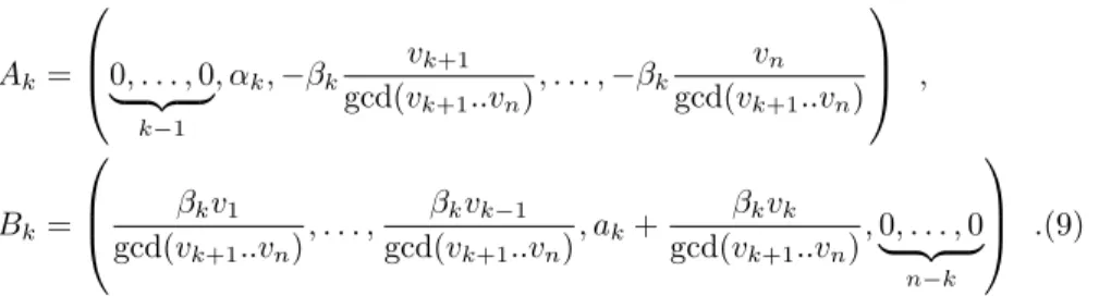
Two antecedents of jk can be obtained by: Ak=   0, . . . , 0_{& '( )} k−1 , αk,−βk vk+1 gcd(vk+1..vn), . . . ,−βk vn gcd(vk+1..vn)    , Bk=   _gcd(vβkv1 k+1..vn) , . . . , βkvk−1 gcd(vk+1..vn) , ak+ βkvk gcd(vk+1..vn) , 0, . . . , 0 & '( ) n−k    .(9)

Projection Matrix. Any point M(a1, . . . , an) in L is projected on the

hy-perplane to a point p(M) = M! _{with integer coordinates (b}

1, . . . , bn−1) in the

(j1, . . . , jn−1) basis. The preimage of M! is the set of points in L that are aligned

with M relative to the projection direction V . These points can be reached from the known point b1A1+ . . . + bn−1An−1:

p−1(M!) = {m|p(m) = M!_{} =} . b1A1+ . . . + bn−1An+ k V gcd(v1..vn) , k_{∈ Z} / . (10) (A1, . . . , An−1, V / gcd(v1..vn)) is a basis of the initial lattice L. An extra row

corresponding to the direction of the projection is added:

A = 0 A1| . . . |An−1| V gcd(v1..vn) 1 =           α1 0 . . . 0 _gcd(vv_1..v1 _n) −β1_gcd(vv2_2..vn) α2 ... ... −β1_gcd(vv3_2..vn) −β2_gcd(vv3_3..vn) ... 0 ... ... αn−1 gcd(vvn−11..vn) −β1_gcd(vvn_2..vn) −β2_gcd(vvn_3..vn) . . .−βn1_gcd(vv_n−1n _{,vn) gcd(v}vn_1..vn)           . (11) P = [Idn−1|0].A−1 . (12)

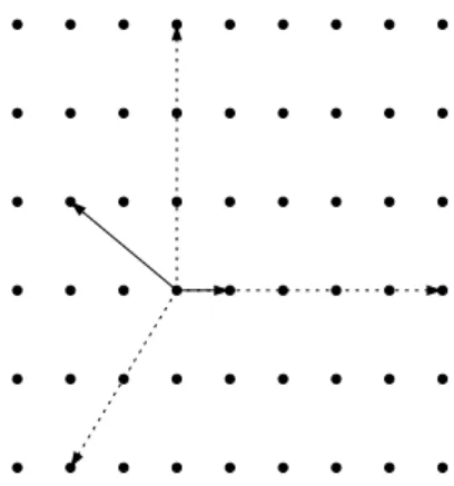
Figure 3 pictures the results of our algorithm for a simple 3D to 2D projection of angle direction (6, 10, 15). The projection matrix is given by:

P = 0 5 6 −6 0 3 −2 1 , and A =  −1 0 6−2 1 10 −3 1 15   .

Fig. 3. The result of the projection of a 3D lattice with angle direction (6, 10, 15). The three dashed lines vectors represent the projection of the initial 3D basis vectors whereas the two plain lines vectors are the result of the computed lattice

3.2 From (n − 1)-Dimension to m-Dimension

To go from a n-dimensional space to a m-dimensional space (m ≥ 1), there are (n − m) projection directions V : V =    v1,1 . . . v1,n ... ... vn−m,1. . . vn−m,n    . (13)

The described method is followed along the first direction:

V1= [v1,1 . . . v1,n] , (14)

and gives the transformation of the basis (i1, . . . , in) to (j1, . . . , jn−1). Each

Vi, i∈ {2, . . . , (n−m)} is projected onto (j1, . . . , jn−1). They give the projection

directions in the (n − 1)-dimensional space with the (j1, . . . , jn−1) basis. The

process is iterated to reach a m-dimensional space.

4

The Projection Matrix

We will define the projection matrix from a n-dimensional space onto a m-dimensional space on the regular grid defined before.

To obtain the final projection matrix, the projection directions can be fol-lowed in different order. One projection direction is chosen, the other projection directions are projected following this first direction and the projection matrix following this direction is derivated. In the projected direction, an other direc-tion is chosen and the same process is iterated. Finally the projecdirec-tion matrix

from the n-dimensional space to the m-dimensional space is obtained by putting together the intermediate matrix.

To go from a n-dimensional space to an m-dimensional space (m ≥ 1), there are (n − m) projection directions Vk.

To obtain the projection matrix from a n-dimensional to an m-dimensional space we will calculate the projection matrix step by step by lowering the di-mension. The final nD to mD projection matrix is composed by products of all the projection matrices describing hyperplane lattices. This matrix being the product of integer matrices has only integer coefficients.

5

Conclusion

Tiling a discrete projected space from higher dimensional Euclidean spaces was the subject of this paper. We first demonstrated how to obtain a tile in a (n − 1)-dimensional space from the Euclidean hypercubic grid of dimension n. The generalization across dimensions is quite straightforward. The obtained results are directly useful for discrete Radon transforms.

References

1. Jeffrey Hoffstein, Jill Pipher, Joseph H. Silverman: NTRU A Ring-Based Public Key Cryptosystem. in Algorithmic Number Theory (ANTS III), Portland, OR, June 1998, J.P. Buhler (ed.), Lecture Notes in Computer Science 1423, Springer-Verlag, Berlin, 1998, 267-288.

2. John H. Conway and N.J.A. Sloan: Sphere Packings, Lattices and Groups. Springer(1998)

3. Harris, J.W., Stocker, H.: Handbook of Mathematics and Computational Science. Springer(1998)

4. Aldroubi, A., Unser, M: Sampling procedures in function spaces and asymptotic equivalence with Shannon´s sampling theory. Numer. Funct. Anal. and Optimiz. 15(1994)1–21

5. Unser, M., Aldroubi, A., Eden, M.: Polynomial Spline Signal Approximations: Fil-ter Desing and Assymptotic Equivalence with Shannon´s Sampling Theorem. IEEE Transaction on Information theory 38(1992)95–103

6. Gu´edon, JP., Bizais, Y.: Separable and radial bases for medical image processing. SPIE lmage Processing 1898(1993)652–661

7. Gu´edon, JP., Bizais, Y.: Bandlimited and Haar Filtered Back-Projection Reconstuc-tion. IEEE Transaction on Medical Imaging 13(1994)430–440

8. Gu´edon, J.P., Unser, M., Bizais, Y.: Pixel Intensity Distribution Models for Filtered Back-Projection. Conference Record of the 1991 IEEE Nuclear Science Symposium and Medical Imaging Conference