A Real Options Analysis of TransEuropean Telecommunications Wireline Video Deployment

Texte intégral

(1)2012s-25. A Real Options Analysis of TransEuropean Telecommunications Wireline Video Deployment Marcel Boyer, Éric Gravel. Série Scientifique Scientific Series. Montréal Septembre 2012. © 2012 Marcel Boyer, Éric Gravel. Tous droits réservés. All rights reserved. Reproduction partielle permise avec citation du document source, incluant la notice ©. Short sections may be quoted without explicit permission, if full credit, including © notice, is given to the source..

(2) CIRANO Le CIRANO est un organisme sans but lucratif constitué en vertu de la Loi des compagnies du Québec. Le financement de son infrastructure et de ses activités de recherche provient des cotisations de ses organisations-membres, d’une subvention d’infrastructure du Ministère du Développement économique et régional et de la Recherche, de même que des subventions et mandats obtenus par ses équipes de recherche. CIRANO is a private non-profit organization incorporated under the Québec Companies Act. Its infrastructure and research activities are funded through fees paid by member organizations, an infrastructure grant from the Ministère du Développement économique et régional et de la Recherche, and grants and research mandates obtained by its research teams. Les partenaires du CIRANO Partenaire majeur Ministère du Développement économique, de l’Innovation et de l’Exportation Partenaires corporatifs Autorité des marchés financiers Banque de développement du Canada Banque du Canada Banque Laurentienne du Canada Banque Nationale du Canada Banque Royale du Canada Banque Scotia Bell Canada BMO Groupe financier Caisse de dépôt et placement du Québec Fédération des caisses Desjardins du Québec Financière Sun Life, Québec Gaz Métro Hydro-Québec Industrie Canada Investissements PSP Ministère des Finances du Québec Power Corporation du Canada Rio Tinto Alcan State Street Global Advisors Transat A.T. Ville de Montréal Partenaires universitaires École Polytechnique de Montréal HEC Montréal McGill University Université Concordia Université de Montréal Université de Sherbrooke Université du Québec Université du Québec à Montréal Université Laval Le CIRANO collabore avec de nombreux centres et chaires de recherche universitaires dont on peut consulter la liste sur son site web. Les cahiers de la série scientifique (CS) visent à rendre accessibles des résultats de recherche effectuée au CIRANO afin de susciter échanges et commentaires. Ces cahiers sont écrits dans le style des publications scientifiques. Les idées et les opinions émises sont sous l’unique responsabilité des auteurs et ne représentent pas nécessairement les positions du CIRANO ou de ses partenaires. This paper presents research carried out at CIRANO and aims at encouraging discussion and comment. The observations and viewpoints expressed are the sole responsibility of the authors. They do not necessarily represent positions of CIRANO or its partners.. ISSN 1198-8177. Partenaire financier.

(3) A Real Options Analysis of TransEuropean Telecommunications Wireline Video Deployment * Marcel Boyer†, Éric Gravel ‡. Résumé / Abstract L’objectif de ce cahier est de montrer comment la méthodologie des options réelles peut être appliquée pour évaluer les projets d’investissement de TransEurope Communications (TEC). Bien que réaliste, l’investissement considéré ici est purement fictif. La conclusion principale de l’exercice est à l’effet qu’on ne peut pas concevoir une stratégie d’investissement optimale si on n’évalue pas de manière explicite la flexibilité managériale de façon appropriée. Mots clés : évaluation des investissements, télécoms, options réelles, flexibilité managériale.. The goal of this paper is to demonstrate how the RO methodology can be applied to evaluate TransEurope Communications (TEC) investment projects. Although realistic, the business case analysed here is fictional. The main conclusion and lesson of this exercise is: One cannot determine a value maximizing investment strategy if one does not value managerial flexibility in an appropriate way. Keywords: investment evaluation, telecoms, real options, managerial flexibility.. *. The goal of this paper is to demonstrate how the Real Options methodology can be applied to evaluate TransEurope Communications (TEC) investment projects. Although realistic, the business case analysed is fictional. † Emeritus Professor of Industrial Economics and CIRANO, Université de Montréal, marcel.boyer@cirano.qc.ca ‡ Economist, Statlog Consulting..

(4) Contents 1 Executive Summary. 1. 2 The Business Case of TEC WV Deployment 2.1 The Sources of Uncertainty and Flexibility . . . . . . . . . . 2.1.1 The Sources of Uncertainty . . . . . . . . . . . . . . 2.1.2 The Sources/Points of Flexibility . . . . . . . . . . . 2.1.3 The Importance of Considering Uncertainty and Flexibility . . . . . . . . . . . . . . . . . . . . . . . . . .. . . .. 6 7 8 8. .. 9. 3 A Simple Example of the Option “Waiting to Invest”. 11. 4 The 4.1 4.2 4.3 4.4. 15 16 20 23 28. Real Options Valuation The Symbols and the Sources of Uncertainty . . . . . . The Footprint Expansion and WV Deployment Project Determination of the Base Case Parameter Values . . . Results and Sensitivity Analysis . . . . . . . . . . . . .. . . . .. . . . .. . . . .. . . . .. 5 Concluding remarks on the RO valuation, Competition, Strategic Planning, and Implementation Issues 38 A A Diagrammatic Representation of Real Options 43 A.1 Diagrammatic Representation for the Current Case . . . . . . 45. i.

(5) 1. Executive Summary. The goal of this paper is to demonstrate how the RO methodology can be applied to evaluate TransEurope Communications (TEC) investment projects. Although realistic, the business case analysed here is fictional. We focus on the consumer side of a footprint expansion and wireline video (WV) deployment for the Berlin area. This project encompasses the following steps: (1) the expansion of the footprint to enable the deployment of WV (including the development of the technology necessary to offer WV), (2) the deployment of WV which requires the completion of the preceding step and (3) the possible addition of a value added service (VAS). The main elements we have identified to evaluate this investment are: the capital expenditures (CAPEX) for the footprint expansion and the WV technology development, the CAPEX for the WV and VAS deployments, the operating expenditures (OPEX) for the supply of WV and the VAS, the monthly revenue per subscriber for WV and the VAS and the number of subscribers for WV and the VAS. Furthermore, we assume that a competitor is currently offering video, voice and data transmission services (not identical to TEC) and that TEC is losing voice and data subscribers by not offering the complete bundle of services (video, voice and data). Among the aforementioned elements, we consider that the main sources of uncertainty are: (1) the CAPEX required for the WV and VAS deployments, (2) the monthly revenue per subscriber for WV and the VAS and (3) the number of WV and VAS subscribers. Furthermore, we assume that the duration of the cash inflows from WV and the VAS is random because technological improvements will eventually render the current technology obsolete. The technology is obsolete in the sense that a better standard becomes available. We make use of a Geometric Brownian Motion (GBM) to model the evolution of the WV and VAS CAPEX. The interesting characteristic of 1.

(6) GBMs is that they can represent many real/empirical phenomena with only two parameters: one for the trend and one for the volatility around this trend. A GBM is also used to model the evolution of the monthly revenue per subscriber. For the number of subscribers in the Berlin area, it is not appropriate to use a GBM. In fact, one expects that the number of subscribers will initially be low and that it will have a tendency to converge to an equilibrium level. To reproduce such a phenomenon, it is appropriate to use a mean reverting process which replicates the desired behavior without excluding random shocks. To model the arrival of obsolescence we make use of a Poisson process. At each moment there is a certain probability (constant for a given interval) that the technology will become obsolete. When the technology becomes obsolete, there is a phasing out period during which subscribers progressively migrate towards the new standard and therefore revenues do not immediately fall to zero. Contrary to the NPV, the strength of the RO methodology lies in its capacity to account for the optimal management of flexibility under uncertainty. For this project, three sources/points of managerial flexibility are immediately apparent: (1) the flexibility to delay the footprint expansion and WV technology development, (2) the flexibility to realize or not and to delay the WV deployment and (3) the flexibility to realize or not and to delay the introduction of a VAS. We present a numerical analysis illustrating the application of the RO methodology to the current project. For matter of simplification and without loss of generality, we shall not consider the option of deploying a VAS in this paper,1 but rather only the option of expanding the footprint and deploying WV will be analyzed. For this, two RO models will be considered; these 1. We will add this non negligeable feature in a future paper.. 2.

(7) are: (1) the option to deploy WV is a European option2 and the decision to expand the footprint or not must be taken immediately; (2) the option to deploy WV is a European option and the option to invest in the footprint expansion is an American option. In this context, a European option reflects the flexibility of realizing (or not) a subsequent step at a given fixed date and therefore optimal timing to exercise the option is not considered. For example, in the first RO model, when it decides to invest in the footprint expansion, TEC purchases or acquires a European option, namely the option to deploy or not WV, an option which can be exercised only after the first investment is completed. In a sense, the footprint expansion is the cost of the real option to deploy later on the WV service. In contrast, the NPV implicitly assumes that if TEC decides to expand its footprint, WV will be deployed notwithstanding market conditions at the end of the first step. In the second model, the option to expand the footprint is an American option in the sense that TEC can decide to realize the footprint expansion at any time within a given period. Because the goal of this study is to demonstrate how the RO methodology can enhance TEC current investment valuation practices, we shall compare the RO valuations with the NPV valuations. In order to determine the base case values for the model’s parameters, we conducted a exchange session with TEC experts in different fields such as technology, marketing, sales and finance, through TEC Business Decision Support Group (BDS). Following this meeting, we determined that: the time to complete the first step (the footprint expansion) is equal to 9 months and costs 206M; the time needed to deploy WV once the first step is completed is equal to 1 year at an expected cost of 181M (random variable); the number of subscribers (random variable) in the Berlin area who would currently be willing to purchase WV services is 38 000; the expected long term equilibrium 2. A European option can be exercised at a given fixed date while an American option can be exercised at any time before its expiry date.. 3.

(8) number of subscribers in the Berlin area is equal to 1.12M; the expected value of the monthly revenue (random variable) per subscriber is 45/month; TEC will make a markup of 40% on WV services; the expected lifetime of the technology (random variable) is equal to 10 years. We assume that 15% of WV subscribers are voice and data protect subscribers and that 35/month in net revenues per voice and data protect subscribers is kept by offering WV services. Note that a 15 % discount rate is used.3 For the base case, we find that it is optimal to realize the first step immediately (expand footprint and start developing WV technology) because the NPV (482.43M) and the value of the first RO model (482.43M) are superior to the value of the second RO model (476.13M) which considers the flexibility of waiting to invest at any time within a given period (0.5, 1 or 2 years). The cost of forgone cash-flows during the delay period exceeds the benefit of waiting for more favorable market conditions. Moreover, we find that in this case, the flexibility of not investing after the end of the first phase (captured by the first RO model) has no value because it is very unlikely that the WV CAPEX will exceed the expected value of the cash-flows from WV. In addition to the base case valuation, we consider five other cases to examine how changes in the parameters affect the value of the project. We find that the optimal investment strategy can vary significantly with changes in the parameters. For example, if we suppose that the long term equilibrium number of subscribers in the Berlin area is equal to 0.6M with the other parameters left unchanged, we find that even though the NPV and the value of the first RO model is positive, it is optimal to wait before realizing the first phase. If we reduce the expected lifetime of the technology from 10 to 6 3. Currently, a theoretically more appealing method called certainty equivalent valuation (CEV) is gaining ground in RO analysis. The difference between the risk adjusted discount rate and CEV is that with the latter, we adjust for risk at the source of risk (stochastic state variables) and we discount the certainty equivalent cash-flows at the riskless interest rate.. 4.

(9) years with an equilibrium number of subscribers of 0.6M, the NPV and the value of the first RO model become negative. However, because the value of the second RO model is positive, the project has value and it should not be discarded on the basis of its negative NPV. TEC should then wait before investing in footprint expansion but keep the project alive because there is high enough probability that the business environment will eventually favour investment. In this situation, TEC must periodically reassess the state of the market, rerun the model and see if the time to invest has arrived. The main conclusion and lesson of this exercise is: One cannot determine a value maximizing investment strategy if one does not value managerial flexibility in an appropriate way.. 5.

(10) 2. The Business Case of TEC WV Deployment. In the current document, we shall focus on the consumer side of a footprint expansion and wireline video (WV) deployment for Berlin. In its simplest version, the project encompasses the following steps. 1. Expansion of the footprint to enable the deployment of WV (this step includes starting the development of the technology necessary to offer WV). 2. The deployment of WV which requires the completion of step 1. 3. The possible addition of one or more value added services (VAS) which requires the completion of steps 1 and 2.4 Based on internal TEC documents and on discussions with TEC BDS group, the main elements we have identified to evaluate this investment are the following. 1. The capital expenditures (CAPEX) for the footprint expansion and the WV technology development. 2. The CAPEX for the WV and VAS deployments. 3. The operating expenditures (OPEX) for the supply of WV and the VAS. 4. Both the number of subscribers and the monthly revenue per subscriber for WV and the VAS. 4. Examples of such VAS are: VoD (Video on Demand), D-PVR (Digital - Personal Video Recorders), home services, VoIP (Voice over IP), gaming, security and other interactive services in addition to broadcast video.. 6.

(11) We assume that a competitor is currently offering a service similar (not identical) to WV and that this competitor is also offering voice and data transmission services (also not identical to TEC services). Accordingly, we suppose that consumers can be divided into the following three groups. A. The consumers preferring to purchase WV services from TEC and willing to wait until the service is available, note that these consumers will not change providers for their voice and data transmission services; B. The consumers preferring to purchase WV services from TEC and who are currently purchasing video, voice and data transmission services from the competitor, if TEC decides to offer WV, these consumers will switch and purchase all three services from TEC; C. The consumers who are currently purchasing voice and data services from TEC and who are willing to switch and purchase all three services (voice, data and video) from the competitor if TEC does not offer WV, if TEC offers WV, these consumers will remain with TEC for all three services (revenue protect).. 2.1. The Sources of Uncertainty and Flexibility. In order to build an appropriate RO model for a particular investment, one must start by identifying the project’s underlying sources of uncertainty and the underlying sources or points of flexibility. These are the model’s main ingredients. In accomplishing this exercise, the decision maker must strike the right balance between practicality and realism. If the model is too complex, it may be difficult to solve and if it is too simple, a bad representation of reality may be given and wrong decisions can end up being made. In this section, we shall identify the main sources of uncertainty and points of flexibility for the project described in the preceding section. This 7.

(12) will be followed by a short valuation example to demonstrate how uncertainty and flexibility are combined to structure and solve a RO problem. 2.1.1. The Sources of Uncertainty. The first source of uncertainty is the level of CAPEX required for the WV and VAS deployments and our understanding is that the volatility in these costs stems from both input cost and technological uncertainty. For given equipment specifications, input cost uncertainty affects the price of building the equipment whereas technological uncertainty stems from the unknowns surrounding final equipment specifications. The second source of volatility is the level of revenues from WV and VAS; these revenues are the product of the number of subscribers and the monthly revenues per subscriber. We assume here that both the number of subscribers and the revenues per subscriber are uncertain. The third source of uncertainty concerns the duration of the cash inflows from WV and the VAS. The duration is random because technological improvements will eventually render the current technology obsolete.5 Finally, we assume for matter of simplicity that the level of CAPEX needed to expand the footprint and to start the development of the WV technology is known and that the OPEX are a deterministic known percentage of revenues. 2.1.2. The Sources/Points of Flexibility. For this project, three sources/points of flexibility are immediately apparent. 1. The flexibility to delay the footprint expansion and WV technology development. 5. The technology is obsolete in the sense that a better standard becomes available.. 8.

(13) 2. The flexibility to realize or not and to delay the WV deployment. 3. The flexibility to realize or not and to delay the introduction of VAS. The above sources of flexibility confer to TEC the option of realizing or not and delaying an investment; for each stage, the decision maker must decide between: 1. investing or abandoning; 2. postponing the decision to the next period (if possible). 2.1.3. The Importance of Considering Uncertainty and Flexibility. Contrary to the NPV, the strength of the RO methodology lies in its capacity to account for the optimal management of flexibility under uncertainty. If management can modify its course of action with the arrival of new information, discounting a single average scenario or predetermined course of action can give a misleading indication of the project’s value. In fact, if we employ the NPV rule (even in its simulated form) for decision making purposes, we can only consider two courses of action, these are: 1. invest if the NPV is superior to zero; 2. reject the project if the NPV is smaller than or equal to zero. If there is uncertainty and it is possible to postpone the investment, the strategy prescribed by the aforementioned rule may be suboptimal. Let’s see why. First, even though the NPV is positive, it may be optimal to wait before investing. In fact, if the NPV is “barely” positive, the manager may want to wait and gain more insurance about the profitability of his project. With 9.

(14) the option of waiting to invest, the decision maker can temporarily avoid embarking in an adventure that presents a high turnaround risk (positive but low initial NPV). The value of the option of waiting to invest (timing option) is positively related to the level of uncertainty in the value of the project and to the irreversibility of CAPEX. If the investment is totally reversible, it is not necessary to wait in order to diminish the probability of a negative turnaround; perfect reversibility implies that capital can be transferred without costs to more profitable activities.6 When the NPV is initially positive, the cost of waiting is equal to the cash flows that would otherwise be realized if the project were operational. The real options methodology enables the manager to assess the optimal trade-off between waiting and investing. In the second case, the initial NPV can initially be negative but the option to wait can still be valuable; in the future, a favorable turnaround can render the investment opportunity interesting (positive NPV). As a result, it is important not to abandon the project before its expiration date even if the current NPV is negative. It is important to note that the value of the option to wait can be zero if strategic considerations force the firm to act rapidly to preempt competition. In a strategic environment, the real options methodology has to be combined with a game theoretic analysis. Finally, other sources of flexibility may potentially exist, for now, we will only consider the flexibility of waiting to invest.7 6 It is important to mention that the reusability of capital is not a sufficient condition for reversibility. Even if capital is reusable, it may be impossible to recuperate invested sums if the capital is industry-specific. The capital’s resale value may be tightly connected to current industry conditions; this makes other potential users also willing to divest and/or unwilling to invest in adverse conditions. 7 An interesting analogy can be made between a project that has a negative NPV with the option to wait and an out of the money call option on a share of stock. This parallel. 10.

(15) 3. A Simple Example of the Option “Waiting to Invest”. As mentioned in the previous section, to undertake an investment, the NPV rule requires that the expected discounted value of a project’s net cash-flows be positive. Under uncertainty, the NPV rule is satisfactory only if one of the following conditions is satisfied: 1. the manager can later reverse his decision and recuperate his original investment at a negligible cost; 2. the investment is a now or never proposition. If the first condition is fulfilled, we say that the investment is perfectly reversible and it is not difficult to imagine situations in which this first condition is violated. Consider an investment in an optical fibre network. It is hard to imagine that the network can be closed and dismantled without loosing a substantial part of the original investment. If the manager has the option to delay, we must not ignore the possibility of realizing the project at a subsequent date when market conditions may be more favorable than presently. For example, consider the opportunity to irreversibly invest  = 1 600 in a project that cannot be altered once it is operational.8 In addition, permits in some way to validate the idea that a project can still have value even though its NPV is currently negative. For example, on September 15 2004 at 11:33AM a share of Verizon Communications (VC) common stock was trading for 39.98US$. At the same time, one could purchase for 1US$ call options to buy one share of VC stock at a strike price of 42.50US$ anytime before April 2005. The NPV of the call option is the difference between the current share price and the option’s strike price, this gives -2.52US$. Even though the option’s NPV is currently negative, the option has a value of 1US$ because there is a probability that before April 2005 the VC stock will rise above 42.50US$. 8 It is straightforward to draw a parallel between this generic project and the opportunity to deploy a VAS.. 11.

(16) suppose that one year after the initial investment , the asset starts producing 1 million units of a good and we assume that the price of this good will evolve according to figure 1. Figure 1 provides us the following information.. Figure 1: Evolution of the Output Price. 1. The uncertainty surrounding the price of the firm’s output is totally resolved after year 2 ( = 2). For example, if the price falls to 2 = 415 it will remain at that level forever. 2. The price of the output in year 0 ( = 0) is known (0 = 166). 3. Starting from each point (state), the two possible price changes have a 50% chance of occurring. For example, if 1 = 83, there is a 50% probability that it will rise to 2 = 1245 and a 50% probability that it will fall to 2 = 415. 4. The expected value at  = 0 of the price  (denoted by 0 [ ]) for. 12.

(17) each period  is equal to 166, that is 0 [1 ] = 05 · 249 + 05 · 83 = 166 0 [2 ] = 05 · (05 · 3735 + 05 · 1245) +05 · (05 · 1245 + 05 · 415) = 166 We assume that in periods 0 and 1, the firm can either invest or postpone the decision to the next period and the discount rate is equal to 10%. If one ignores the fact that the investment is irreversible and that it is possible to wait, he will invest immediately because  0 = −1 600 +. ∞ X 166 =1. (11). = 60  09. However, if the manager considers the option to wait before investing, his time  decision will be based on the following criterion:  = max {   }  where  is equal to the value of investing immediately and  is the value of waiting; those values are determined below. To compare the  = 0 value of the dynamic and static strategies, a simple dynamic programming argument will be used. Even though this example is simplified, the solution method used is very similar to those employed to resolve more complex American option problems. Referring to figure 1, because the market is stable after  = 2 there is no point in delaying the investment past  = 2, the project becomes a now or never proposition. If the manager has not yet invested, the optimal decision is to invest if 2 = 3735 because the NPV is equal to  2 = −1 600 + 9. ∞ X 3735 −2 = 2 135 (11) =3. Remember that at  = 0, the expected cash flow for every period is equal to 166.. 13.

(18) and to abandon if 2 = 1245 or 415 because  2  0. Going back one period ( = 1), if the manager has not yet invested, he then has to decide either to invests at  = 1 or to wait until  = 2. Let us compare the value of both strategies: if 1 = 249 (this price corresponds also to the expected price for   1), then the value of investing immediately is equal to 1 =  1 = −1 600 + and the value of waiting is equal to " Ã ( 1. ∞ X 249 −1 = 890 (11) =2. )! ∞ X 3735 + = 05 · max 0 −1 600 + (11)−2 =3 )!# Ã ( ∞ X 1245 1 · 05 · max 0 −1 600 + −2 (11) (11) =3 = [05 · (2 135) + 05 · (0)] ·. 1 (11). = 97045 if 1 = 83 (this price corresponds also to the expected price for   1), the NPV is negative and it will always be negative because 2 can only equal 1245 or 415.10 Consequently, if 1 = 249, it is optimal to wait another period. The manager should then invest at  = 2 if and only if 2 reaches 3735. Let us now consider the optimal decision at  = 0. We determined above that  0 = 0 = 60. If the manager decides to wait, the value of waiting is equal to 0 = [05 · max {1 if 1 = 249 1 if 1 = 249} +05 · max {1 if 1 = 83 1 if 1 = 83}] · = [05 · (97045) + 05 · (0)] · 10. 1 (11). 1 = 44111 (11). To compute the value of 1 , we calculated the discounted expected value of the  = 2 optimal investment strategy.. 14.

(19) At  = 0, because 0  0 , it is optimal to wait until the next period before making a decision. In the next period ( = 1), we determined above that if we have not yet invested, then the optimal strategy is to postpone the decision to the next period ( = 2). Consequently, the strategy that gives the highest expected value at  = 0 is to wait till  = 2 and invest if and only if 2 reaches 3735.. 4. The Real Options Valuation. We mentioned in the preceding section that to build a RO model, the first crucial steps were to identify the sources of uncertainty and the sources/points of flexibility. We then emphasized the importance of considering the interaction between uncertainty and flexibility when valuing an investment. Finally, a simple example was given to show that considering flexibility can alter a manager’s decision. In this section, we shall bring together the project specific elements described previously and build the RO model for the footprint expansion and wireline video (WV) deployment for Berlin. To do this, we will make use of several tools. First, to enlighten the presentation, symbols will be used to represent the variables and parameters entering the model.11 Second, the evolution of the sources of uncertainty will be modelled by using different types of stochastic processes, the main characteristics of these processes will be described. Third, we will describe the RO model for the footprint expansion and WV deployment project. Note that in this model, the type B and C consumer categories will be merged and their number will be expressed as a percentage of total consumers. This is the case because the effect on incremental revenues 11 Contrary to a variable, the value of a parameter does not change with time, it is constant throughout the model.. 15.

(20) of type B and C consumers is the same. Finally, in order to design a RO model, it is useful to lay out a diagram of the firm’s decision process in both its state-of-the-system space and its time space. To build these diagrams, different building blocks are used. In appendix A the different building blocks are described and a diagrammatic representation of TEC decision process will be given.. 4.1. The Symbols and the Sources of Uncertainty. From here on, the letter  will be used to represent time in years with  = 0 indicating current time and  designates the risk adjusted discount rate. The other symbols used to represent the model parameters are given in Table 1. Table 1: Parameter Definitions Symbol Definition  1   2   3 time to complete first three phases, respectively 1  2. time limit to delay footprint expansion and VAS deployment, respectively. . CAPEX for first phase (footprint expansion).   . units of capital for WV and VAS deployments, respectively.   . variable cost multiples for WV and VAS, respectively. . percentage of type B and C consumers. . net monthly revenues from data and voice. . VAS revenue multiple. 16.

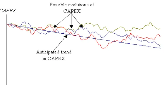
(21) CAPEX As we mentioned, the level of CAPEX for the WV and VAS deployments is stochastic. For tractability, we assume that the same random factors (input cost and technological) will affect the level of CAPEX for both services. This is a reasonable assumption if we expect that the same type of components are used for both technologies and that their development presents similar technical challenges. Because of this, a single Geometric Brownian Motion (GBM) may be used to model the evolution of the cost per unit of capital which we denote as  (). To determine the level of CAPEX at a date  for a particular service, we multiply the cost per unit of capital ( ()) by  or  . For example at , the cost of deploying WV and the VAS will be equal to  ·  () and  ·  (), respectively. The interesting characteristics of GBMs is that they can represent many real/empirical stochastic phenomena with only two parameters: one for the trend and one for the volatility around this trend.12 Figure 2 shows three possible CAPEX patterns that were generated by a GBM with a declining trend. A declining trend can be used to account for the fact that many telecommunications and information technology equipment costs tend to fall over time as a result of technological improvements and increasing competition between suppliers. A positive trend is used to model the evolution of prices that have a tendency to rise (in real terms). 12. For example, if we expect CAPEX ¡ to ¢ decrease by 2% per year with a volatility of 20%, the percentage change in CAPEX ∆ in one year can be expressed as:  ∆ = 002 + 020 ·  . where  is a draw from a standard normal distribution.. 17.

(22) Figure 2: Evolution of CAPEX Monthly Revenue Per Subscriber We also use a GBM to represent the evolution of the monthly revenues per subscriber  (). Note that the monthly revenue per subscriber for the VAS is a multiple of the monthly revenue per subscriber for WV, using the symbols of table 1, the monthly revenues from the VAS at time  are equal to  ·  () (compared to  () for WV). Number of subscribers For the number of subscribers in the Berlin area, denoted by  (), it is not appropriate to use a GBM. In fact, one expects that the number of subscribers will initially be low and that it will have a tendency to converge to an equilibrium level . To model such a phenomenon, it is appropriate to use a mean reverting process which replicates the desired behavior without excluding random shocks. Figure 3 illustrates mean reversion in  () for an initial number of 18.

(23) subscribers that is lower than the long term equilibrium value . The expected evolution of the number of subscribers curve illustrates the expected convergence phenomenon, the number of subscribers is expected to grow in a stochastic or volatile way, at a positive but decreasing rate towards . The possible paths illustrated on Figure 3 and the 95% confidence interval for subscribers illustrates the randomness of the process. We suppose that all WV subscribers will subscribe to the VAS.. Figure 3: Evolution of the Number of Subscribers Obsolescence Finally, we model the arrival of obsolescence with a Poisson process, at each  there is a certain probability (constant for a given interval) that in the next instant the technology becomes obsolete. When the technology becomes obsolete, there is a phasing out period where subscribers progressively migrate towards the new standard, revenues do not fall to zero immediately.. 19.

(24) 4.2. The Footprint Expansion and WV Deployment Project. In this section we propose two RO models which differ according to their degree of flexibility. In both models, the monthly incremental cash-flows from WV at time  is equal to the monthly revenue per subscriber for WV times the number of subscribers and the markup on WV services plus the net revenues on voice and data times the number of type B and C consumers. For the VAS, the monthly incremental cash-flows at time  is equal to the monthly revenue per subscriber for VAS times the number of subscriber and the markup on the VAS. Note that the duration of the cash-flows for both WV and the VAS is stochastic because of the possibility of obsolescence.13 The first model In the first model, we assume that all of the options embedded in the project are European. In this context, a European option reflects the flexibility of realizing (or not) a subsequent step at a given date, optimal timing is not considered. For example, if TEC decides to expand the footprint at  = 0, it buys the European option of deploying WV at  =  1 and the value of this option stems from the possibility of obtaining cash-flows from WV at  =  1 +  2 plus the European option to add a VAS at  =  1 +  2 . In this first model, the first decision TEC has to take is whether or not to invest  at  = 0 to expand the footprint. After the expansion is terminated (in  1 years), TEC must decide whether or not to deploy WV. If TEC decides to deploy WV, it must invest  ·  ( 1 ) at  =  1 and this service will start generating revenues at  =  1 +  2 (this includes incremental revenues 13. Mathematically, the monthly incremental revenues at time  for WV and VAS are respectively equal to:  ()  () (1 −  ) +  ()   and  ()  () (1 −  ) . 20.

(25) from type B and C consumers). The third decision TEC has to take after completing the WV deployment (at  =  1 +  2 ) is either to invest  ·  ( 1 +  2 ) to add the VAS or not, in which case TEC only receives the revenues from WV. The VAS will start generating revenues at  =  1 + 2 + 3 . Note that from  = 0 to  =  1 +  2 +  3 , the random variables keep fluctuating according to changes in the business environment and there is always a possibility that the technology becomes obsolete. If the technology becomes obsolete, subsequent investments will not be made and no additional cash-flows will be realized. For example, if the technology becomes obsolete before  =  1 , WV and the VAS will not be deployed and  will be lost. In the above model, the value of investing  stems from the European options to deploy WV and the VAS. At this point, it is important to contrast this model with a simulated NPV approach. According to NPV, when  is invested, it is implicitly assumed that all subsequent investments will be made notwithstanding the future state of the market. Consequently, the decision maker is discounting the expected cash flows of a predetermined course of action. In contrast, the European option model considers that subsequent investments will be made only if they are profitable at that future point in time. The second model For the second model, we suppose that TEC has the option to delay the footprint expansion during some period of time 1 . This option is of the American type, that is, TEC can invest  at anytime between  = 0 and  = 1 to acquire the European options to deploy WV and the VAS. Compared to the previous case, TEC has the flexibility of waiting for more favorable market conditions before investing . If the project has a negative NPV at  = 0, it is possible that a favorable turnaround will render the investment attractive and therefore TEC must then consider keeping the. 21.

(26) option alive.14 For matter of simplification and without loss of generality, we shall not consider the option of deploying a VAS, but rather only the option of expanding the footprint and deploying WV will be analyzed. Hence the two RO models considered are: 1. Model 1: the option to deploy WV is European and the decision to expand the footprint or not must be taken immediately; 2. Model 2: the option to deploy WV is European and the option to expand the footprint is American (TEC can decide to invest  in footprint expansion at any time during a period of length 1 ). The Expected NPV Because the goal of this study is to demonstrate how the real options methodology can enhance TEC current investment valuation practices, we shall compare the RO valuations to those computed according to the NPV rule. To compute the expected NPV, we first determine the discounted expected value of the WV cash-flows and we deduct of this amount the discounted expected value of the WV CAPEX and . This is consistent with traditional NPV analysis as we implicitly assume that once  is invested, all subsequent investments (deployment of WV) will be made notwithstanding market conditions at  =  1 . We use a risk adjusted discount rate of 15% to compare the NPV results with the RO results. However, a theoretically more appealing method called certainty equivalent valuation (CEV) is gaining ground in RO analysis. The difference between the risk adjusted discount rate and CEV is that with the latter, we adjust for risk at the source of 14. In a waiting to invest context, keeping the option alive means doing what is necessary (information updates, meetings, etc.) to eventually reconsider investing in the project.. 22.

(27) the risk (stochastic state variables) and we discount the certainty equivalent cash-flows at the riskless interest rate. All of the aforementioned sources of uncertainty are considered including obsolescence. Furthermore, note that the timing of obsolescence can result in two types of outcomes. First, if the technology becomes obsolete before  =  1 , WV will not be deployed and only  will be lost. Second, if obsolescence occurs after WV is deployed, we suppose that revenues at the date of obsolescence will gradually phase out. In this example, we assume that revenues at the date of obsolescence will have a half-life of one year.15. 4.3. Determination of the Base Case Parameter Values. As mentioned, to determine the base case values for the model’s parameters, we conducted a meeting analogous to the IVA sessions organized by TEC BDS group. It is important to mention that the simulated IVA session that we held gave us “ball park” figures and in reality, more information (if possible) should be obtained to supplement and validate this first pass. The questions that were asked (and the answers) are the following: • Questions relative to step 1 1. How much time will it most likely take to complete the first step of the project (expansion of footprint and development of the WV technology) for the Berlin area? That is, upon starting the first step, in how many months can TEC be ready to start the WV deployment? Answer: The expected time to complete the first step is 9 months, consequently, we have  1 = 075 15. If revenues have a half-life of one year, then they will be down to 50% of what they were at obsolescence one year after obsolesence, down to 25% after two years, down to 12.5% after three years, etc... 23.

(28) 2. What amount will most likely need to be invested to complete step 1 (to get the network ready to start WV deployment) for the Berlin area? Answer: This amount is equal to 206M, this includes the investment necessary to get the network ready plus the cost of starting the development of the WV technology, consequently, we have  = 206. • Questions relative to step 2 3. Once the network is ready, how much time will it most likely take to deploy WV for the Berlin area? Note that at the beginning of the second step, only the necessary bandwidth is available and the WV technology is assumed developed. Answer: The expected time span between the start of WV deployment and the reception of cash flows from WV is equal to 1 year, consequently, we have  2 = 1 4. As seen from today, what amount would most likely need to be invested to realize the second step (in  1 years)? That is, starting from raw bandwidth and a developed WV technology, how much would TEC need to invest to have WV available in the Berlin area? Answer: As seen from today, by the time TEC is ready to deploy wireline video (in 9 months), the expected cost is 181M. Note that the BDS group consider a 2% growth factor to account for expected real changes in this type of costs. Consequently,  = 002 (expected growth rate of CAPEX) and if we suppose that  (0) = 1, we have  ·  (0) = 181−002·075 ' 178 ⇒  = 178 5. With 95% confidence, what are the highest and lowest values for the cost of deploying WV in 9 months? 24.

(29) Answer: The 95% confidence band is estimated to be ± 10 to 15 percent of the starting 178M cost. With this information we estimate that   (volatility parameter of CAPEX) is between 0.05 and 0.10. 6. Assume that WV is available today. How much revenues (the revenues variable is equal to the number of subscribers times the annual revenue per subscriber) would TEC most likely get from it in the next year? Answer: In its first year of availability, it is expected that 38 000 households in the Berlin area will subscribe to wireline video, it is also expected that the average revenue per household will be 45 per month, consequently, the expected initial monthly revenue is equal to 1.71M. Note that no growth is expected in the average revenue per household, consequently,  = 0,  (0) = 45 and  (0) = 0038. 7. With 95% confidence, what are the highest and lowest values for the average monthly revenue per subscriber in 1 year and 9 months? Answer: The 95% confidence band is estimated to be ± 15 percent of the 45 figure provided in the previous answer. With this information we estimate that   (volatility parameter of monthly revenue per subscriber) is around 0.06. 8. We expect that the number of WV subscribers will grow during part of the lifetime of the product. However, we think that the number of subscribers will start relatively low and that it will converge to a constant long term number of subscribers. What would be the most likely long term equilibrium number of subscribers? Answer: The most likely long term equilibrium number of subscribers is estimated at 1.12M (28% share of the 4M households in Berlin), con25.

(30) sequently,  = ln (112) = 01133 (logarithm of long term equilibrium number of subscribers). 9. In how much time do you expect that the growth rate will converge to its long term value? Answer: It is expected that by 2010 WV will have reached its equilibrium penetration rate (we suppose that the study starts in 2004). It is difficult only with this information to estimate  (mean reversion rate). For this, we will consider the average time it takes for the current spread between the actual and the equilibrium number of subscribers to be reduced by half (from 38 000 subscribers to 579 000 subscribers), for different average times, we have the following table:. Average time κ 1 1.63 2 0.82 3 0.54. According to the above table and the answer to the current question, the most plausible value for  is 0.82. 10. With 95% confidence, looking ahead to 2010, what are the highest and lowest values for the number of subscribers in the Berlin area? Answer: By 2010, with 95% confidence the number of subscribers will be between 0.6M and 2M, consequently with  = 163,   (volatility parameter for the number of subscribers) should be approximately equal to 0.55. 11. Suppose that two types of costs must be incurred to offer WV: the first 26.

(31) type of costs is positively related to revenues (variable costs) and the second is independent of revenues and it must be incurred to keep on offering WV in the Berlin area (fixed costs). i. Suppose that WV is available to a customer that hasn’t yet subscribed. If this customer decides to subscribe, what are the costs to TEC of serving this customer on an ongoing basis? Can this be expressed as a percentage of revenues per customer? Answer: We suppose that variable costs are 60% of monthly revenues (markup of 40% often used by economic study group), consequently,  = 06. ii. What is the most likely annual recurring fixed cost of keeping WV available in the Berlin area, independently of demand? Answer: We suppose that these costs are included in the initial investment cost. • Question related to the technology 12. What is the expected lifetime of the WV technology? Answer: As seen from today, the expected lifetime of the technology is 1 as the base 10 years. Consequently, we will consider a value of  = 10 case value. Finally, we suppose for the base case that the number of type B and C consumers is equal to 15% of type A consumers ( ()) and that the net monthly revenue from data and voice services is equal to 35.. 27.

(32) 4.4. Results and Sensitivity Analysis. The difference between the first model (the option to deploy WV is European and the decision to expand or not the footprint must be taken immediately) and the expected NPV is that in the first model we explicitly take into account the fact that TEC will deploy WV only if market conditions at  =  1 justify the investment. Instead of discounting the expected value of a single predetermined course of action (like in the traditional NPV approach), we discount the expected value of an optimal course of action which is to invest if and only if the NPV of WV at  =  1 is positive. We label the value computed from the first model as NPV-RO-1. For the second model (the option to deploy WV is European and the option to expand the footprint is American), we add the possibility of choosing the date of the footprint expansion investment during a period of length 0.5 year, 1 year, or 2 years. We label the value computed from the second model as NPV-RO-2.16 In addition to the base case valuation, we include five other cases to examine how changes in the parameters affect the value of the project and the differences between valuation methods. Furthermore, for each case, we give the following informations: 1. The value of the parameters (Tables 2.X where X stands for the case number considered); 2. The 95% confidence intervals for the stochastic variables at  =  1 (Tables 3.X) and the expected value of the cash-flows from WV (EVCFWV) evaluated at the lower bound of the 95% intervals for the number of subscribers ( ()) and the monthly revenues per subscriber for WV ( ()) at  =  1 (conditional on the technology not being obsolete at 16. Note that the value NPV-RO-2 is computed conditional on not having invested at  = 0.. 28.

(33)  =  1 ). Because  () and  () are independently distributed and that the EVCFWV is increasing in  () and  (), there is a 95.1% probability that the EVCFWV will be superior to the one evaluated at the lower bounds of the 95% confidence intervals for the number of subscribers ( ()) and the monthly revenues per subscriber for WV ( ()). 3. The valuation results for the NPV, the NPV-RO-1 and the NPV-RO-2 (Tables 4.X). Note that after case 1, (base case) the tables are always up updated from the previous case. The Computation of RO-Valuations For both RO models (NPV-RO-1 and NPV-RO-2), the first step consists in computing the EVCFWV at the date WV is operational ( 2 years after TEC decides to deploy WV) conditional on the technology not yet being obsolete. To do this, we start by calculating the EVCFWV for a general cash-flow duration of  and we then take the expectation of this EVCFWV with respect to the distribution of  . Note that the distribution of  is determined by  (expected lifetime of the technology). The second step is to establish the EVCFWV at the date TEC decides to deploy WV ( 1 years after TEC decides to expand the footprint). In this case, we take the expected discounted value of the EVCFWV found in the first step, considering that the technology can become obsolete in the interval of time ( 2 ) it takes to deploy WV. The third step for the NPV-RO-1 model is to take at  = 0 the expected value of the optimal investment strategy (WV deployment) in  1 years. In this case, we proceed by Monte-Carlo simulation, the steps are: 1. Generate a large number of trajectories (10 000 or more) for the value 29.

(34) at  1 of: (1) the number of subscribers, (2) the monthly revenue per subscriber for WV and (3) the WV CAPEX; 2. Compute the second step EVCFWV conditional on the  1 values generated in the previous step; 3. For each trajectory, take the maximum between (i) the EVCFWV at  1 minus the WV CAPEX and (ii) zero, discount that maximum back to  = 0 and weight it by the probability that the technology will not become obsolete in the interval of time  1 ; 4. Sum the values for each trajectory, divide by the number of trajectories and deduct  to obtain NPV-RO-1. Finally, to compute NPV-RO-2 we proceed in the same spirit as in the section A Simple Example of the Option “Waiting to Invest”. In this case, the value of investing immediately is equal to the value computed in the third step for the NPV-RO-1 and we determine by backward induction the optimal investment date and the value of NPV-RO-2. Note that while we wait, it is also possible that the technology will become obsolete. Case 1 (base case) We have the following tables for case 1:. 30.

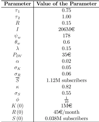
(35) Table 2.1: Parameters for Case 1 Parameter Value of the Parameter 1 0.75 2 1.00  0.15  206M 178   0.6  0.15  35  0.02  0.05  0.06  1.12M subscribers  0.82  0.55 1  10  (0) 1M  (0) 45/month  (0) 0.038M subscribers The 95% confidence intervals are: Table 3.1: Confidence Intervals at τ 1 for Case 1 Variable Lower bound  ( 1 ) 165.83M  ( 1 ) 40.59/month  ( 1 ) 0.09M subscribers. Upper bound 196.51M 49.76/month 0.37M subscribers. The EVCFWV evaluated at the lower bounds of the 95% confidence intervals for the number of subscribers ( ( 1 )) and the monthly revenues per subscriber for WV ( ( 1 )) is equal to 885.55M. The valuation results are:. 31.

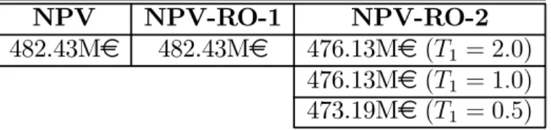
(36) Table 4.1: Valuation Results for Case 1 NPV NPV-RO-1 NPV-RO-2 482.43M 482.43M 476.13M (1 = 20) 476.13M (1 = 10) 473.19M (1 = 05) In this case, because the NPV is superior to the NPV-RO-2 for all length 1 ’s, it is optimal to start the footprint expansion (invest ) immediately. The cost of forgone cash-flows during the delay period exceeds the benefit of waiting for more favorable market conditions. Moreover, notice that the NPV and the NPV-RO-1 are equal; by simply comparing the EVCFWV (885.55M) to the upper bound of the confidence interval for  ( 1 ) (equal to 196.51M), we see that it is very unlikely that  ( 1 ) will exceed the EVCFWV. As seen from  = 0, the optimal strategy at  1 will probably always be to invest. Consequently, the flexibility of not investing at  1 if market conditions are poor does not have any value in this case. Case 2 In case 2, we suppose that the equilibrium long term market penetration () is equal to 0.8M subscribers (compared to 1.12M subscribers for case 1). This changes the  1 confidence intervals for  ( 1 ). We have the following tables for case 2 (update of case 1): Table 2.2: Parameters for Case 2 Parameter Value of the Parameter  0.8M subscribers The 95% confidence intervals are:. 32.

(37) Table 3.2: Confidence Intervals at τ 1 for Case 2 Variable Lower bound  ( 1 ) 0.08M subscribers. Upper bound 0.31M subscribers. The EVCFWV evaluated at the lower bounds of the 95% confidence intervals for the number of subscribers ( ( 1 )) and the monthly revenues per subscriber for WV ( ( 1 )) is equal to 642.79M. The valuation results are: Table 4.2: Valuation Results for Case 2 NPV NPV-RO-1 NPV-RO-2 251.80M 251.80M 247.83M (1 = 20) 247.74M (1 = 10) 247.63M (1 = 05) As in case 1, the optimal decision is to start the footprint expansion immediately (NPV  NPV-RO-2 for all 1 ). Furthermore, by comparing the EVCFWV (equal to 642.79M) to the upper bound of the confidence interval for  ( 1 ) (equal to 196.51M), the same can said about the equality between NPV and NPV-RO-1. Case 3 In case 3, we suppose that the equilibrium market penetration () is equal to 0.6M subscribers (compared to 0.8M subscribers for case 2). This changes the  1 confidence intervals for  ( 1 ). We have the following tables for case 3 (update of case 2): Table 2.3: Parameters for Case 3 Parameter Value of the Parameter  0.6M subscribers The 95% confidence intervals are: 33.

(38) Table 3.3: Confidence Intervals at τ 1 for Case 3 Variable Lower bound  ( 1 ) 0.07M subscribers. Upper bound 0.27M subscribers. The EVCFWV evaluated at the lower bound of the 95% confidence interval for the number of subscribers ( ( 1 )) and the monthly revenues per subscriber for WV ( ( 1 )) is equal to 487.73M. The valuation results are: Table 4.3: Valuation Results for Case 3 NPV NPV-RO-1 NPV-RO-2 105.80M 105.80M 109.34M (1 = 20) 109.34M (1 = 10) 109.34M (1 = 05) Here even if NPV and NPV-RO-1 are both positive, it is optimal to wait before investing because the value of NPV-RO-2 is superior for all 1 . However, the values of NPV-RO-2 are identical for all 1 ; extra time to wait past 0.5 years does not add any value to the investment. This phenomenon can be explained by the small difference (3.35%) between NPV-RO-1 and NPV-RO-2. In fact, the small difference signals that a slight improvement in market conditions would be sufficient to trigger the investment; the expected time it takes to attain the threshold at which the cost of waiting becomes superior to the cost of foregone cash-flows should be in the interval  = 0 and  = 1 = 05, so that having the extra flexibility of a larger 1 is of no value. The best strategy for TEC is to wait, rerun the model in  years (1 month 1 years) with 1 = 05 −  and see if NPV-RO-1 (or NPV) is is equal to 12 superior to NPV-RO-2, if not, wait again and repeat. Finally, the same as in cases 1 and 2 can be said about the equality between NPV and NPV-RO-1.. 34.

(39) Case 4 In case 4, we reduce the expected lifetime of the technology from 10 years to 6 years, while the value of the other parameters are as in case 3. We have the following tables for case 4 (update of case 3): Table 2.4: Parameters for Case 4 Parameter Value of the Parameter 1  6 There is no need to update table 3.3 (confidence intervals for case 3). The EVCFWV evaluated at the lower bound of the 95% confidence interval for the number of subscribers ( ( 1 )) and the monthly revenues per subscriber for WV ( ( 1 )) at  =  1 is equal to 370.66M. The valuation results are: Table 4.4: Valuation Results for Case 4 NPV NPV-RO-1 NPV-RO-2 -10.96M -10.96M 18.92M (1 = 20) 14.51M (1 = 10) 7.79M (1 = 05) In case 4, both the NPV and the NPV-RO-1 are negative. If TEC does not have the option to wait, market conditions at  = 0 do not justify the investment. However, if TEC can wait before investing, there is a probability that the business environment will eventually favor investment and as compared to case 3, there is a value in having extra time to wait past 0.5 years. Finally, the same as in cases 1, 2 and 3 can be said about the equality between NPV and NPV-RO-1.. 35.

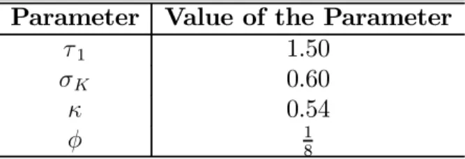
(40) Case 5 For case 5, many parameters have been changed: the time to complete the first phase ( 1 ) is increased from 0.75 to 1.50 years, the volatility parameter for WV CAPEX is increased from 0.06 to 0.6, the mean-reversion factor is reduced from 0.82 to 0.54 and the expected lifetime of the technology is equal to 8 years. We have the following tables for case 5 (update of case 4): Table 2.5: Parameters for Case 5 Parameter Value of the Parameter 1 1.50  0.60  0.54 1  8 The 95% confidence intervals are: Table 3.5: Confidence Intervals at τ 1 for Case 5 Variable Lower bound  ( 1 ) 33.16M  ( 1 ) 39.84/month 0.07M subscribers  ( 1 ). Upper bound 591.16M 50.64/month 0.44M subscribers. By examining table 3.5, we see that the 95% confidence interval for  ( 1 ) is much wider than in the previous cases: two factors account for this difference. First, it takes more time to complete the footprint expansion and to develop the WV technology and therefore, everything else being equal, there is more uncertainty the further we look ahead. Second, the value of the volatility parameter has been increased by a 10-fold factor. Both of these changes have been done to illustrate that there can be a difference between the NPV and the NPV-RO-1. The valuation results are: 36.

(41) Table 4.5: Valuation Results for Case 5 NPV NPV-RO-1 NPV-RO-2 -3.55M 3.53M 45.31M (1 = 20) 36.31M (1 = 10) 26.48M (1 = 05) In this case, there is a difference between the NPV and the NPV-RO-1. The  = 0 value of the WV investment opportunity computed according to the NPV is equal to 202.45M and the one computed by considering that TEC has the option to invest or not at  1 is equal to 209.53M. Using 200 000 trajectories to compute NPV-RO-1, we found that 4.65% of the trajectories result in the EVCFWV being inferior to  ( 1 ) compared to 0.00% in the previous cases. Finally, even though NPV-RO-1 is superior to 0, the optimal strategy is to wait and gain more assurance concerning the profitability of the project. In addition, a longer time to wait has more value. Case 6 In case 6, we reduce the proportion of type B and C consumers from 15 % to 0.00%. We have the following tables for case 6 (update of case 5): Table 2.6: Parameters for Case 6 Parameter Value of the Parameter  000 There is no need to update table 3.5 (confidence intervals for case 5). The valuation results are:. 37.

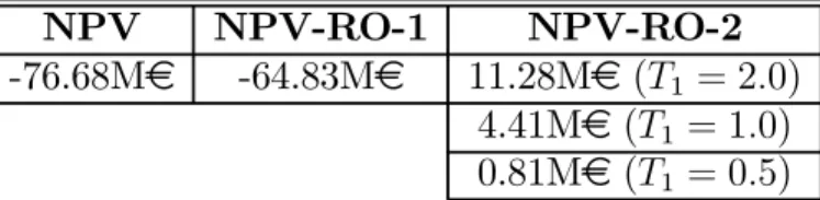
(42) Table 4.6: Valuation Results for Case 6 NPV NPV-RO-1 NPV-RO-2 -76.68M -64.83M 11.28M (1 = 20) 4.41M (1 = 10) 0.81M (1 = 05) Compared to case 5, the difference between the NPV approach and the NPV-RO-1 has increased. Using 200 000 trajectories to compute NPV-RO-1, we found that 9.19% of the trajectories result in the EVCFWV being inferior to  ( 1 ) compared to 4.65% in the previous case. As in case 5, the option of waiting to invest is quite valuable.. 5. Concluding remarks on the RO valuation, Competition, Strategic Planning, and Implementation Issues. To show the potential of the RO valuation methodology as a complementary tool in defining an optimal value maximizing investment strategy for TransEurope Communications (TEC) , we retained six evaluation scenarios of the WV deployment project, which provide an interesting array of outcomes. Many other scenarios with different parameter combinations could of course be analyzed. First, the study shows that the value maximizing strategy is not always to wait, that is, the NPV can sometimes give the right answer (cases 1 and 2). Second, it illustrates that if one has to pay for extra flexibility, it may not always be a good idea to do so. For example, scenario 3 shows that if one can purchase extra time to wait, it may not be optimal to do so. Third, scenarios 1 to 4 show that if one can obtain more favorable condi38.

(43) tions from suppliers by committing to invest in the future, the value of the flexibility given up may be negligible. Fourth, the optimal investment strategy can vary significantly with changes in the parameters. Hence, the value maximizing strategy may be to invest immediately and in others it may be to wait until business conditions are more favorable either to diminish the probability of a negative turnaround that will render the investment unprofitable or to allow a possible positive turnaround which will make a currently unprofitable investment profitable. The main conclusion and lesson is: One cannot determine the value maximizing investment strategy if one does not value managerial flexibility in an appropriate way. Strategic Competition There seems to be a necessity to introduce WV before a cable company (CC) deploys voice over the internet protocol (VoIP). TEC considers that if it does not deploy WV before the CC deploys VoIP, the CC will temporarily offer a voice, video and data bundle that will cause TEC to lose a significant amount of actual and potential subscribers. We did not explicitly consider competitive interactions between TEC and the CC and its effect on the optimal timing of the footprint expansion. The focus was on the basic modelling process which consists in identifying and combining the sources of uncertainty and flexibility into a RO valuation model. If there is a first mover advantage (FMA), the RO model must be able to assess the optimal trade-off between the value of waiting to invest and acting early to preempt competition. Even if there is a competitive threat, preempting competition does not always dominate waiting. Consequently, one cannot at the outset dismiss the RO value of waiting. To take into 39.

(44) account competitive interactions, the RO methodology must be combined with a game theoretic analysis. For such an endeavour, we need a good understanding of the specific nature of competition. A financial option cannot have a negative value because its owner has the possibility of exercising it, but never the obligation to do so. Nonetheless, one important characteristic of real options in an strategic competitive environment is that a firm may be less valuable if it holds a real option than if it does not. This paradox arises as follows. The value of real options derives from the active management of a project’s steps and variations as uncertainty unfolds over time. However, the possibilities of modifying the planned course of a project imply that the firm’s commitment to develop and eventually complete the project is relatively low. This lack of commitment may invite more aggressive behavior from competitors, whose objective may be to drive the firm out of the project or market, or more aggressive attacks from the opponents to the project. Active management means that such options, although valuable in a competitive non reactive business environment, may not be valuable in an oligopolistic reactive business environment: managers must sometimes burn their bridges. It is a major responsibility of higher level managers to identify which options should be closed in favor of strong commitment and which options should be kept open in favor of flexibility. Strategic Planning A good strategic plan is a plan that builds real options into the foreseeable future of the firm and sets up an optimized decision making process to fruitfully exploit those options. Again, real options should be recognized, built in and evaluated for each major step of every project: alliances, acquisitions and mergers, spin-offs, technology development and management, organizational restructuring, etc. The real options approach considers strategic management and decision-making as a process aimed at actively reducing 40.

(45) exposition to downside risk and promoting exposition to upside opportunities. It stands at the hinge between pure finance and other areas of decision making under risk such as project evaluation, market entry and exit, organizational restructuring and re-engineering, technology adoption, climate change and biodiversity decisions, etc. The value of strategic planning itself is determined by the quality of the real options designed and imbedded in the plan and by the quality of the evaluation procedure of those real options. It is in this precise sense that the design and management of real options, through the exploitation of uncertainty, create value for the firm and that they represent the most important responsibilities of the managers in determining a strategic plan. Strategic planning is an exercise in managing flexibility. Plans should specify decision nodes, that is to say future steps that may or may not be taken, at dates that may be given but are mostly to be chosen optimally as the future environment of the firm unfolds in a stochastic way. Furthermore, preparing a strategic plan is not a passive exercise in anticipating the future; it is an exercise in shaping the future or, more precisely, an exercise in preparing the way, in due time, the future will unfold to the decision maker’s advantage. That is, managers are planting the seeds of future flexibility by identifying and creating real options. This is again a key difference between real options and financial options: with real options, managers are creating the tool or using existing tools in highly creative ways; in the case of financial options financial executives usually pick their tools in the - sometimes highly exotic - kit of available instruments. Implementation The real options methodology is emerging as a potentially powerful tool for the executive. However, this potential will only be realized by decisionmakers who combine the "real option state of mind" with both a good grasp of technical skills and a good information system. The implementation of a real. 41.

(46) options approach could be very valuable but at the same time is a challenging task. The RO approach is relevant to a very large array of management and strategic decisions involving competition, uncertainty, flexibility and irreversibility. However, implementing a real options approach is not easy. Each application of the RO approach is likely to be context specific. The available options must be envisaged and described; the relevant information must be identified and collected carefully; the user of the RO approach must have the required knowledge and training to adapt the standard procedures to each particular situation. This being said, we think that with some training and some strategic support, TEC has the human resources necessary to start implementing the RO approach. Finally, we believe that real options approach has high potential for value creation because the RO methodology is not only a valuation method but also a tool that provides a common language between finance and strategic planning. The approach underlines a frame of mind and uses methodologies that appeal to a wide array of managers, thus providing a common language. Real options have applications in many areas that are central to modern corporations: market coverage and development, finance, human resources management, technology management, R&D and knowledge management, etc. Thinking in terms of real options represents a major development in strategic but remains relatively unknown in spite of its adoption by firms such as Airbus, GE, Hewlett Packard, Intel, Toshiba and others.. 42.

(47) A. A Diagrammatic Representation of Real Options. To build the decision process diagram, we will use a method inspired by Leppard and Cannizzo (2002).17 Each diagram is constructed by combining the following building “blocs”: • Bloc 1: value as a function of the system state:. Bloc 1 This symbol represents the value of an asset as a function of the state variables. In this particular case, the state variables are CAPEX, monthly revenues per subscriber, the number of subscribers and obsolescence and value can be that of the expected cash flows for WV. • Bloc 2: punctual cash-flows:. Bloc 2 A punctual cash-flow does not depend on any future event, sales at a particular instant are an example of punctual cash-flows. 17. Leppard, Steve and Fabio Cannizo (2002), “Diagrammatic Approach to Real Options,” in Ehud I. Ronn (ed.), Real Options and Energy Management: Using Options Methodology to Enhance Capital Budgeting Decisions, Risk Books, London.. 43.

(48) • Bloc 3: Decisional D, probabilistic P and unconditional U transition boxes:. Bloc 3 A probabilistic transition (P) indicates a movement in the stochastic state variable space and it is used to represent the stochastic nature of variables like revenues, CAPEX or obsolescence. For its part, a decisional transition (D) represents a movement in the decision space, for example the passage from the inactive to the investment state. Finally, an unconditional transition is used to link symbols. • Bloc 4: Passing of a known fixed period of time ∆ with discounting at a rate of :. Bloc 4. • Bloc 5: Passing of a period of time that is currently unknown and chosen optimally (can be constrained by a length of time  ) with discounting at a rate of :. Bloc 5 44.

(49) This symbol can be used to denote the time before an “American” option is exercised. • Bloc 6: Result emanating form a transition: Bloc 6. A.1. Diagrammatic Representation for the Current Case. Diagram 1 (parts 1 and 2) positions TEC decision process in the system state and time spaces when all of the options embedded in the project are European. In this context, a European option reflects the flexibility of realizing (or not) a subsequent step at a given date, optimal timing is not considered. For example, at  = 0 if TEC decides to expand the footprint, it buys the European option of deploying WV at  1 . For this model, the system state is characterized by the level of the state variables and by the “contractual” space. The “contractual” space depends on TEC current and past decisions, for example, an element of the “contractual” space can be {expand footprint, deploy WV, abandon the option of deploying VAS}  In part 1 of diagram 1, the first decisional transition (D1 ) marks the passage from the inactive state to the abandon or footprint expansion state. If TEC decides to expand its footprint,  must be invested at  = 0 (indicated after U1 ) and after the expansion is terminated (in  1 years), TEC must decide at D2 whether or not to deploy WV. If TEC decides to deploy WV, it must invest  ·  ( 1 ) at  =  1 and this service will start generating revenues at  =  1 + 2 as indicated in part 2 of diagram 1 (above unconditional transition U5 ). 45.

(50) Figure 4: Diagram 1 (part 1): Decision process when Project Options are of the European Type For its part, the third decisional transition (D3 in part 2 of diagram 1) indicates that after completing the footprint expansion and the WV deployment (at  =  1 +  2 ), TEC must decide either to invest  ·  ( 1 +  2 ) to add the VAS or to abandon and only receive the revenues from WV. The VAS segment will start generating revenues at  =  1 +  2 +  3 .. Figure 5: Diagram 1 (part 2): Decision process when Project Options are of the European Type Note that in each diagram, the probabilistic transitions P denote the 46.