Calculation of the random-incidence scattering coefficients of a sine-shaped surface

Calculation of the random-incidence scattering coefficients

of a sine-shaped surface

Jean-Jacques Embrechts

Department of Electrical Engineering and Computer Science Université de Liège, Belgium

Lieven De Geetere, Gerrit Vermeir

Laboratory of Acoustics and Laboratory of Building Physics Katholieke Universiteit Leuven, Belgium

Michael Vorländer

Institute of Technical Acoustics RWTH Aachen University , Germany Tetsuya Sakuma

Institute of Environmental Studies University of Tokyo, Japan Summary

Random-incidence scattering coefficients obtained by measurement in reverberation chambers (ISO 17497-1) are compared with theoretical results. Holford-Urusovskii’s method and a hybrid plane wave decomposition - FEM method are applied to infinite periodical surfaces, while the Kirchhoff approximation and 3D BEM give numerical results for finite-size surfaces. The validity of the computations is compared and discussed with regard to the approximations involved. Finally the applicability and reliability of the measurement method is evaluated by comparison with the most appropriate approaches. Although the measured scattering coefficients are slightly higher than expected from the calculations, the measurement method seems to yield reliable data to be used in ray tracing or other prediction models.

PACS 43.55.Br, 43.55.Mc Short title: Sine-shaped surface scattering calculations

Contact author:

Jean-Jacques Embrechts

Department of Electrical Engineering and Computer Science

University of Liège, Sart-Tilman B28

B-4000 Liège 1, Belgium mailto: jjembrechts@ulg.ac.be Tel: ++32-(0)4 366 2650 Fax ++32-(0)4 366 2649 Received revised accepted

1. Introduction

The scattering properties of surfaces are more and more considered in room acoustics, especially when the sound field distribution or the reverberation in an architectural space are analysed. Recently, measurements methods for determination of the “scattering coefficient” and the “diffusion coefficient” were developed and standardised, respectively by ISO [1] and AES [2].

The scattering coefficient is defined as the ratio of the non-specularly reflected power to the total acoustic power reflected by the surface. In particular, the random-incidence scattering coefficient is defined for a perfectly diffuse incident sound field. The importance of the use of the random-incidence scattering coefficient in room-acoustical computer simulations is already known [3,4,5].

In a former publication [6], the authors of this paper have compared several measurements of the random-incidence scattering coefficient of a sine-shaped surface. These measurements were performed in real-size reverberation rooms, as well as in scale models, according to the ISO method [1]. Among others, this study aimed at testing the reliability, accuracy and robustness of this method, by comparing measurements results obtained in three different laboratories.

At the same time, it was also intended to compare these measurements results with theoretical values of the random-incidence scattering coefficients, calculated for the same sine-shaped surface. It is the purpose of this paper to report on the theoretical results computed by several methods, to discuss and compare them with measurements results and to draw conclusions about the reliability of the ISO measuring technique.

2. Surface scattering: a short review of theoretical methods

2.1. Rough surfaces

Several theoretical methods have been used to analyse the sound waves reflected by a corrugated surface. Most of them are approximations, in the sense that they give reliable results if and only if some assumptions are satisfied. These assumptions may be related to the incident wave (most often a monochromatic plane wave, conditions on the wavelength, the angle of incidence), to the surface itself (finite or infinite, perfectly rigid or pressure release surface, surface impedance) or to the roughness profile (periodic or random, conditions on the average height or slope).

It is not intended here to write an extensive review of all these methods, but well to find theoretical results to which our measurements on the sine-shaped surface sample could be compared. More detailed reviews can be found in [7,8,9], for example.

Following Thorsos and Broschat [8], there are two classical methods to solve the theoretical problem of the scattering by a rough surface: the small perturbation method (SPM, sometimes called Rayleigh or Rayleigh-Rice approximation) and the Kirchhoff approximation (KA). Beyond these two classical methods, more recent theories have been set up to extend the domain of validity. Among them is the “small slope approximation” or SSA [8,10,11].

The small perturbation method relies upon Rayleigh’s original work [12], in which a periodic surface (a sine-shaped one in that case) is shown to generate, above the rough surface, a reflected sound pressure field represented by a sum of outgoing plane waves. Rayleigh’s hypothesis consists in assuming that this representation also holds inside the corrugations of the surface, which allowed him to find the amplitudes of these outgoing waves, and therefore to solve the scattering problem (Dirichlet condition: p=0).

It has been shown that Rayleigh’s hypothesis is valid for slightly rough surfaces (height of the corrugations, h, much less than the surface wavelength, Λ). For a sine-shaped surface, the ratio h/Λ must be less than 1/14 [13,14], but Wirgin [13] showed that ratios up to 0.34 were acceptable. Furthermore, there’s also a condition on the wavelength of the incident sound wave, i.e. kh<4.1 [13]. Both conditions are satisfied by our sine-shaped surface profile (for frequencies up to 8700 Hz), but these conditions have been derived for pressure-release conditions (p=0 on the surface). For our surface, Neumann boundary conditions (perfectly rigid surface) rather hold.

In the following, the Holford-Urusovskii’s method [14] will be developed, taking into account Neumann boundary conditions. This method gives an exact solution, indicating that

Rayleigh’s assumption is not necessary, but it is required that the surface should be periodic and, therefore, infinite.

Another way of avoiding Rayleigh’s hypothesis is to split the fluid domain into two sub-domains by an imaginary plane lying on the top of an infinite periodical surface [15]. A plane wave decomposition (PWD) still applies for the infinite outside domain, and the FEM is used inside the domain limited by the imaginary plane and one period of the rough surface. We will show results obtained with this hybrid FE-PWD method up to 8 kHz.

In this paper, the KA method will also be applied. This method starts from the Helmholtz integral expression of the sound field scattered by a finite-size rough surface [16], relating the far-field pressure in any direction to the pressure and its gradient on the rough surface. These last values are then estimated by their tangent-plane expression, which leads to the solution of the surface integral. The Kirchhoff or tangent-plane approximation holds for “sufficiently smooth” surfaces, for which the local radii of curvature exceed the wavelength [7,17]. The KA method has mainly been developed for random surfaces [7,16,17], but it is also valid (under the same kind of conditions) for deterministic surfaces, in particular periodic or flat ones.

BEM methods are also efficient to find the sound field distribution around a finite-size scatterer at low frequencies. These methods also solve the Helmholtz surface integral problem, but without requiring any approximation. The scattering surface has to be discretized into several sub-elements which should be smaller than the wavelength. The compromise between the size (upper frequency limit) and the number (computing time and memory requirements) of elements is a well-known problem. To face this problem, efficient algorithms have been proposed for very thin plates or periodic surfaces [18,19]. In this paper, 3D BEM results up to 2 kHz will also be obtained for our sine-shaped surface.

2.2 Rigid plate

The ISO method for measuring the scattering coefficient is a two-step method. Scattering by a circular plate (the upper surface of the turntable) is first measured [1], then a test sample with

the same circular shape and external diameter is laid down on the turntable and scattering is measured again. Some numerical methods used in this paper to calculate the scattering coefficient of the sine-shaped surface will also need to evaluate the sound field scattered by a circular rigid plate.

This problem has already been investigated by several authors: see for example [21,22,23]. One of their conclusions is that the scattered field is made of two contributions: the reflected (specular) wave and the sound diffracted by the edges. It also appeared that no general (analytical) solution could be found for this (apparently) simple problem.

In the absence of general solutions, scattering by the rigid disc will be evaluated in this paper by the methods that use Mommertz’ correlation technique [16,20] to obtain the scattering coefficient, i.e. the KA and the 3D BEM methods. Reliable predictions require that the results be computed in the far field, a condition being particularly important for the Kirchhoff

approximation [22].

3. The test surface

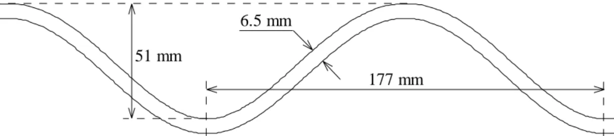
The reference test surface is the same sine-shaped surface that was used for the laboratory measurements reported in [6]. The dimensions of this surface are recalled in figure 1. Not shown is the 3m diameter circular shape of the sample. It is obvious that the reflection of sound waves on a surface of this shape will be strongly angle-dependent and that this surface is not applicable to create random diffusion in room acoustics. In this study it only serves as a reference for comparison purposes.

6.5 mm

177 mm 51 mm

Figure 1: Dimensions of the test sample: structural wavelength Λ = 177 mm, structural depth = 51 mm.

4. Results obtained by the Holford-Urusovskii’s method

4.1. Description of the method

In 1981, R.L. Holford proposed an exact solution for the problem of the scattering at an infinite periodic surface [14]. In this publication, the case of a pressure-release surface is developed, but the more general impedance boundary condition is treated in an appendix, which is referred as “Urusovskii’s method” [24].

This method has been applied to our sine-shaped surface, which is of course periodic. The impedance boundary condition is expressed by a zero normalized admittance in Holford’s equation (A1), since the surface is here perfectly rigid. This assumption is justified by the relatively weak absorption coefficient of our sample. There’s no a priori condition of validity for the application of this method. However, the size of the surface must be infinite, which represents a significant difference with our sample.

Despite this difference, it was decided to compute Holford-Urusovskii’s solution and to compare this solution with the measured values of the random-incidence scattering coefficients. One reason is that the ISO procedure is defined to give measurements results which should represent an infinitely large surface, even if the test sample has itself finite dimensions. This could be verified by applying Holford-Urusovskii’s method. Another reason is that the diameter of the sample is much greater than the wavelength for most frequencies of interest.

The detailed operations of this method are described in [14, Appendix A]. Only a short summary is recalled in the following. However, some particular developments have required more extensive work, since their derivation from Holford’s paper was not really obvious. These particular developments are also mentioned in the following.

The sound field reflected by infinite periodic surfaces can be expressed by a sum of plane waves. If axis Ox is taken perpendicular to the sine-shaped corrugations and Oz perpendicular to the mean plane of the surface (see fig. 2), and if the incident plane wave vector lies in the (Ox,Oz) plane, then the reflected sound field does not depend on “y” :

Λ + = =

∑

+∞ −∞ = +

φ

λ

α

γ α n z x _n n z x jk n refl

R

e

p

n n 0 ( cos , ) , ( ) for z>ξmax (1)

In this equation, φ0 is the angle of incidence measured from Ox and Rn is the undetermined

complex amplitude of plane wave number n. Two cases must be distinguished in the sum (1): if abs(αn)<1, then the nth plane wave is a radiating wave in direction φn (see fig. 2) given by :

φ

γ

φ

α

φ

λ n n n n cos , n sin cos 0+ Λ = = = (2)

otherwise, it is an evanescent surface wave.

Holford-Urusovskii’s method of course consists in finding the values of the undetermined amplitudes Rn, in particular for the radiating waves which are the only ones that scatter energy

in the far field. The amplitude R0 corresponding to the radiating wave n=0 is the specular

component. Therefore, as the surface is assumed to be perfectly reflecting, the scattering coefficient is, by definition :

2 0 0, ) 1 (φ k = −R

δ (3)

The total fraction of energy reflected in the far field is the sum of the contributions of all radiating modes :

∑

= waves radiating n n R sin sin 0 1 2 φ φ (4)

For frequencies less than (c/2Λ), the only radiating wave is the specular (n=0) one, whatever the angle of incidence. In the case of our sine-shaped surface, this lower frequency limit is about 960 Hz (c=340 m/s). Therefore, there should be no scattering below this value.

Figure 2: Scattering at a periodic surface, definition of axis and angles.

To find the undetermined amplitudes Rn, Holford starts from the general Helmholtz integral

formulation. In the Helmholtz integral, the total pressure on the rough surface is

calledφ(x)=ptot(x,ξ(x))), and the pressure gradient vanishes since the surface is perfectly rigid.

The periodicity of the rough surface allowed Holford to write the following expression :

∑

+∞ −∞ = = n x jk n

e

n x

φ

α φ( ) (5)

He showed that the coefficients of this series expansion can be found by solving the following (infinite) system of linear equations :

dx x x p

_e

U

inc jk x m n n mn m m α ξ

φ

φ

φ

+∞ Λ − −∞ =

∫

∑

= =_Λ − 0 , ( , ( )) 2 2

ˆ

m=0,±1,±2,_K (6)

In our implementation, this system is truncated to an order Nmax and the coefficients

φ

n are computed through the inverse of matrix (I-U). The difficulty here is that the elements of this matrix have a quite complicated expression, given by eq. (A1) of this paper.

Once the problems of implementation are solved (see appendix), the Holford-Urusovskii’s method can be applied, through the following steps :

1. Given a maximum number of equations (2Nmax+1), solve the system (6);

2. Introduce the coefficients

φ

n in (5) to find the pressure on the surface; 3. Introduce )φ(x in the Helmholtz integral to find the pressure in the far-field.

A shortcut for steps 2 and 3 is proposed (it is valid for z>ξmax, which is the case in the

far-field) :

2’. Compute the amplitudes Rm with Holford’s expression (A19), in which the admittance

η0=0;

3’. Verify eq. (4) for radiating waves only;

4’. Finally, compute the scattering coefficient by (3).

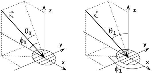
There’s still an important problem to solve if we want to obtain the random-incidence scattering coefficient. Indeed, up to now, eq. (3) only gives the scattering coefficient for an incident wave vector belonging to the plane perpendicular to the sinusoidal corrugations (fig. 2). Again, Holford gives a hint to compute the scattering coefficient for an incident wave vector lying outside this plane. He first defines θ0 as the angle between the incident wave

vector k1and the plane (Ox,Oz), as shown in fig. 3, which gives :

(

0 0 0 0 0

)

1=k cosθ cosφ,sinθ ,−cosθ sinφ

k 0≤φ0≤π −π/2≤θ0≤π/2 (7)

He further proves that the scattered field can still be expressed by a sum of plane waves whose complex amplitudes Rn are those computed for the case θ0=0 with the wavenumber

k’=kcosθ0 .

Again, the reflected wave “n=0” is in the specular direction, which leads to :

) cos , 0 , ( ) cos ( 1 ) , , ( 0 0 0 2 0 0 0 0θ θ δφ θ θ φ δ k= −R k = = k (8)

This expression shows that the scattering coefficient for any incident wave can be deduced from the coefficient computed for the corresponding incident wave perpendicular to the sinusoidal profile, by simply shifting the frequency (the shift factor being cosθ0).

φ

₀

θ

0 y x z k1

φ

₁

θ

₁ y x z k1

Figure 3: Definition of angle θ0 (left) and classical angle description

This conclusion is very important for the computation of the random-incidence scattering coefficient. Indeed, the application of the Holford-Urusovskii’s method can be restricted to that plane θ0=0, and the integration over θ0 is then replaced in the Paris formula [25] by an

integration over frequency. The classical formulation of the Paris formula is (see fig. 3) :

1 2 0 1 1 1 1 2 / 0 1 ( , , )sin cos 1 ) ( _π θ δ θ φ θ θ φ δrand f = π

∫

d

∫

π f d (9)

Changing from (θ1,φ 1) to (θ0,φ 0) gives :

0 0 0 2 0 0 0 2 / 2 / 0 ( , , )sin cos 1 ) ( _π θ δφ θ φ θ φ δ π π π d f d f rand

∫

∫

− = (10)

Taking (8) into account, and integrating over f’= f cosθ0 , finally gives :

∫

∫

⎟ ₋= ⎠ ⎞ ⎜ ⎝ ⎛ = f rand df f f f f f d f 0 2 2 0 0 2 2 / 0 0 0 ' ' ') , 0 , ( ' sin 4 ) ( _π φ φ δ φ θ δ π (11)

This modified Paris formula has been implemented and computed as a weighted sum with 10 degrees step in φ0 and 20 Hz step in frequency (below 4500 Hz) or 50 Hz step (above 4500

Hz).

4.2.Results and discussion

The first results of the Holford-Urusovskii’s method for our sine-shaped surface show the scattering coefficient obtained for directional incident waves, with the incident vector perpendicular to the sinusoidal corrugations (θ0=0°).

Figure 4 illustrates the scattering coefficient for an incident wave at . Clearly, for frequencies less than

° = 04 0 φ

(

c

)

1088Hz cos 1 0 = +

Λ φ , there’s only one radiating mode (n=0), leading to a

scattering coefficient equal to zero. An interesting finding is that, at the frequency at which the mode n=-1 appears at , it contains almost all the reflected energy, and the scattering coefficient suddenly rises to one. Whereas at 2176 Hz, i.e. the frequency at which the mode n=-2 appears at , the mode n=0 seems to carry all the reflected energy again. ° = −1 180 φ ° = −2 180 φ

0.0 0.1 0.2 0.3 0.4 0.5 0.6 0.7 0.8 0.9 1.0 0 1000 2000 3000 4000 5000 6000 7000 Frequency [Hz] Scattering coefficient [-] Nmax=12 Nmax=7 Nmax=4 Nmax=2

Figure 4: Scattering coefficient of the sine-shaped surface for a plane wave incident along φ0

= 40° (θ0 = 0°), and for several values of the parameter Nmax.

This figure also shows that Nmax=7 is the minimal order leading to a correct evaluation of the

scattering coefficient in the whole frequency band of interest (in fact, the curves Nmax=7 and

Nmax=12 coincide perfectly on this graph). This is confirmed by the calculation of the total

reflected energy by eq. (4) which significantly deviates from one above 4500 Hz if Nmax<7.

The same conclusions have been drawn from the computations at φ0= 01 °.

Graphs similar to figure 4 have been computed every 10 degrees step in φ0. Finally, all these

results have been introduced in (11) to obtain the random-incidence scattering coefficient, which is illustrated in figure 5.

0.0 0.1 0.2 0.3 0.4 0.5 0.6 0.7 0.8 0.9 1.0 0 1000 2000 3000 4000 5000 6000 7000 Frequency [Hz] Scattering coefficient [-] Holford-Urusovskii

FE-PWD: 10° step in azimuth and elevation

FE-PWD: 10° step in azimuth and 2° step in elevation

Figure 5: Random-incidence scattering coefficient of the sine-shaped surface computed by the Holford-Urusovskii’s method (10° step in φ0) and by the hybrid FE-PWD method with

directional resolution of every 10° step in φ0, and every 2° or 10° step in θ0.

5. Results obtained by the hybrid FE-PWD method

5.1. Description of the method

Considering an imaginary plane on the top of a sine-shaped surface, it divides the fluid domain into a semi-infinite outside domain and periodic inside ones (see fig. 6). As a

numerical approach, the FEM is applied to the inside domain bounded by the imaginary plane and one period of the surface, while the plane wave decomposition (PWD) is theoretically applicable in the outside domain as described in sections 2.1 and 4.1.

If the incident plane wave vector lies in the (Ox,Oz) plane, the total sound pressure and its gradient on the imaginary plane (z=0 in fig.6) are expressed by:

p_tot,b(x) = ejkxα0+ R ne jkxαn

Σ

n = –∞ +∞ (12) ∂ptot,b(x) ∂n = – jkγ0e jkxα_{0+ (jk}γ n)Rne jkxα_n

Σ

n = –∞ +∞ (13) Subsequently, eq. (13) can be transformed into:

R_n=δ_n0+ 1 jkγnΛ ∂ptot,b(x) ∂n e–jkxαndx 0 Λ (14) Substituting eq. (14) into eq. (12) gives the relationship between the total pressure and its gradient:

ptot,b(x) = 2e jkxα₀₊ e jkxα_n jkγnΛ ∂ptot,b(x′) ∂n e–jkxαndx′ 0 Λ

Σ

n = –∞ +∞ (15) The above equation (which is valid for the imaginary plane) can be discretized to express the boundary condition for the FE modelling in the inside domain :

p_b = f + 1

jk T U qb

(16)

where {pb} and {qb} are the pressure and its gradient at nodes on the imaginary boundary (Nb is the number of nodes), [T] and [U] are matrices of the size (Nb, Nmax) and (Nmax, Nb), respectively.

On the other hand, the FE system for the inside domain is expressed by: K – jk C – k2M p_pin b = M 0 q_b (17)

where [K], [M] and [C] are the stiffness, mass and damping matrices, respectively. This system can be solved, which determines {pin}, {pb} and {qb}. Substituting the sound pressure gradient {qb} into eq. (14) gives the value of R0, and finally, the scattering

coefficient is obtained by eq. (3).

If the incident plane wave vector does not lie in the (Ox,Oz) plane, two simple modifications are required for the plane wave decomposition and for the FE modelling, respectively. In the former, the factors αn and γn must be redefined as :

(

φ

)

_θ

φ

γ

_θ

φ

θ

α

λ n n n

n=cos 0cos 0+nΛ =cos 0cos , =cos 0sin (18)

In the FE system (17), only the frequency conversion from k to k cosθ0 is needed.

in cid en t w av_e mod e n= 0 inside domain imaginary plane outside domain Z X φ0 φ0 n

Figure 6: Division of fluid domain into inside and outside domains by the imaginary plane

(z=0) on a periodic surface.

5.2.Results and discussion

Figure 7 shows the scattering coefficients of our sine-shaped surface computed by the hybrid FE-PWD method and by Holford-Urusovskii’s method, which are obtained for directional incident waves with θ0=0 and φ0= 04 °. In the computation with the hybrid method,

Nmax=100 was given for the plane wave decomposition, and elements of width less than 1/15

wavelength were used for the FE modelling. It is seen in this figure that both curves correspond up to 8 kHz.

Figure 7: Scattering coefficient of the sine-shaped surface for a plane wave incident

alon i’s

The scattering coefficients for directional incident waves have been computed for several

FE-in ts

orrespondence with the Holford-Urusovskii’s method is again observed, which confirms the

. Results obtained by the Kirchhoff Approximation (KA) method

both methods previously applied, it is assumed that the sine-shaped surface is of infinite

0.0 0.1 0.2 0.3 0.4 0.5 0.6 0.7 0.8 0.9 1.0 0 1000 2000 3000 4000 5000 6000 7000 Frequency [Hz] Scattering coefficient [-] Hybrid FE-PWD Holford-Urusovskii

g φ0=40° (θ0 = 0°), computed by the hybrid FE-PWD method and Holford-Urusovski

method

incidence angles θ0 and φ0 and, finally, the random-incidence scattering coefficient was

obtained according to Paris' formula. Figure 5 shows the results obtained with the hybrid PWD method, where the directional scattering coefficients are computed every 10 degrees step in φ0, and every 2 or 10 degrees step in θ0. Apparently, the results with high resolution

θ0 draw a smooth line, and also give slightly lower values at high frequencies. Thus, it is

considered that in this case, 10 degrees step in θ0 is not enough to smooth the high gradien

in the frequency characteristics of directional scattering coefficients due to radiating modes. C

validity of both methods.

6 In

size, which is not the case for the real surface that was tested during our measurements (see section 3). The KA and 3D BEM will allow to take this finite size into account.

6.1. Description of the complete KA method

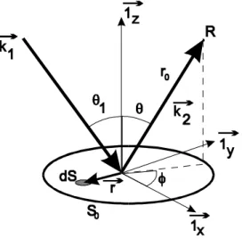
The complex scattered pressure at point R in the far field is [7, eq.(19.18)] :

∫∫

= 0 ) . ( ) ( . S r v j reflR K e v dxdy p γ (19)

In this equation, the sound pressure has been evaluated in the Fraunhofer zone (far field), for an incident plane wave [16]. The geometrical parameters and vectors included in expression (19) are defined in figure 8. In particular, the vector v is the difference between k1

(incidence) and k2 (scattering), both vectors having a magnitude of k=2π/λ, r is the position

vector of the surface element dS with co-ordinates (x, y, z=ξ(x,y)) and γ is a vector

perpendicular to the rough surface at dS, with co-ordinates (-dξ/dx, -dξ/dy,1). Finally, Kis a complex constant inversely proportional to r0, the distance between the point R and the centre

of the rough surface.

Equation (19) is valid for perfectly hard rough surfaces, a condition which is assumed throughout this paper.

Figure 8: Scattering geometry for a plane wave incident along vector k1.

The receiver R lies in the far field along scattering direction k2.

Equation (19) is used to compute by numerical integration the sound pressure scattered by our sine-shaped sample in all directions k2(θ,φ). The roughness profile function to be included in

this equation is ξ(x,y)=Hcos(2πx/Λ), with H=0.0255m and Λ=0.177m (see fig.1).

Once the free-field scattering distribution has been computed, the scattering coefficient can be derived from the Mommertz formula [16,20], for a specified direction of incidence k1.

Finally, the random-incidence scattering coefficient is obtained by numerical integration over all vectors k1, using Paris’ formula.

The procedure is repeated for each frequency of interest, which can lead to particularly long

.2. The “characteristic function” model [16]

s the far-field scattering distribution of the rigid disc reduces to a specular lobe (as long as n computing times. This can be avoided by the following method.

4

A

the radius of the disc is “much greater” than the wavelength), then the Mommertz formula ca be simplified [16], and the following expression is found for the scattering coefficient:

2 ) , ( 1 cos 2 0 1 0 1 1 ) , ( =−

∫∫

− S y x jk dy dx e S k θξ θ δ (20)

In the particular case of our one-dimensional sine-shaped sample, equation (20) reduces to:

2 2 2 ) ( cos 2 2 Re −jk θ1ξx 2 1, ) 1 (

∫

− − − = e R e e dx x R e R k _π θ δ (21)

where Re is the radius of the circular sample (Re =1.5m).

xpression (21) shows that the scattering coefficient δ depends on the direction of incidence E

1

k through angle θ1. Furthermore, it can also be shown that a rotation of the sample in the

ane (x,y) does not change the value of the scattering coefficient computed through this expression. As δ only depends on the elevation (θ1) of the direction of incidence (and not

its azimuth), this greatly simplifies the random-incidence computations through the Paris formula.

pl

on

umerical integration in (21) is carried out with 100 discretization intervals per wavelength

he validity of the “characteristic function” model has been tested in this study by comparing N

(this has been shown to give reasonable accuracy). The results for our sine-shaped sample are shown in figure 9, for several angles of incidence θ1 (from 5 to 85 degrees). Finally, numerical

integration over angle θ1 through the Paris formula gives the random-incidence scattering

coefficient values, which are also illustrated in figure 9. T

some results of figure 9 with those obtained with the classical KA method (19), coupled with the Mommertz formula. Several computations have been carried out, including nine directions of incidence in the plane φ1=0° (perpendicular to the sinusoidal corrugations) and nine in the

plane φ1=90° (parallel to the corrugations). The correspondence between both models was

excellent between 315 and 8000 Hz, as long as the angle of elevation θ1 did not exceed 80

0.0 0.1 0.2 0.3 0.4 0.5 0.6 0.7 0.8 0.9 1.0 125 250 500 1000 2000 4000 8000 16000 Frequency [Hz] Scattering coefficient [-] 5° 15° 25° 35° 45° 55° 65° 75° 85° rand. inc.

Figure 9: Scattering coefficients of the sine-shaped surface computed by the Kirchhoff approximation (“characteristic function” model), for several anglesof incidence θ1, and for

random-incidence.

The validity of the Kirchhoff approximation for the rigid disc as well as for the sine-shaped surface will be discussed later in section 8. It will be concluded that KA results are not reliable enough in this case. This can already be expected from fig. 9 that shows different trends than figs. 4 and 7. In particular, KA predicts that scattering starts at lower frequencies for lower incidence angles θ1. This is contradicted by the Holford-Urusovskii’s and hybrid

FE-PWD methods which show the inverse trend. The finite size of the surface is not responsible for this effect, as will be shown in section 7. On the other hand, the random-incidence results seem to coincide quite well with the previous methods: this is probably due to an “averaging” effect.

Another method is therefore necessary to analyse the finite size effect of the rough surface.

7. Results obtained by the BEM method

As a fourth method, 3D BEM calculations are used to calculate the scattering coefficient for our circular sine-shaped surface using the Mommertz correlation method [16,20]. The indirect boundary integral formulation (infinitely thin surfaces) is chosen in combination with a variational solution scheme, as provided by the software Sysnoise Rev. 5.5 [26]. Therefore, a 3D BEM model of the circular sine-shaped surface and an equally sized flat surface is

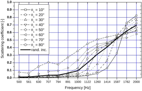
constructed. 2000 Hz was found to be the upper limit for reliable calculations, in relation to the element size of the surface mesh, which is made up of 18786 triangular elements. The receiver mesh is a hemisphere with an elevation and azimuth resolution of 2° and radius of 100 m [27]. Directional scattering coefficients are calculated for incidence angles with a resolution of 10° in azimuth and elevation angle. For each elevation angle, the obtained scattering coefficients can be averaged over all azimuth angles. These averaged directional

scattering coefficients can then be combined using Paris’ formula to obtain the random-incidence scattering coefficients (figure 10).

500 561 630 707 794 891 1000 1122 1260 1414 1587 1782 2000 0.0 0.1 0.2 0.3 0.4 0.5 0.6 0.7 0.8 0.9 1.0 Sc a tte ri n g c o e ffi c ie n t [-] Frequency [Hz] θ₁ = 10° θ₁ = 20° θ₁ = 30° θ₁ = 40° θ₁ = 50° θ₁ = 60° θ₁ = 70° θ₁ = 80° rand. inc.

Figure 10: 3D BEM calculated scattering coefficients of the sine-shaped surface using Mommertz’ correlation method for different elevation angles (averaged over all azimuth

angles) and for random-incidence.

The calculations point out that, as expected, the surface starts to scatter at lower frequencies when the incidence elevation becomes more and more grazing. Due to lobing effects caused by the finite size of the surface, the transition at the frequency at which a first order (n=±1) scattered wave appears, is smoother compared to infinite periodic surfaces. Also interesting to note is the cross-over of the curves at the hinge point around 1600 Hz; from 1782 Hz on, the order of the curves is comparable with the order of the curves in the KA model (figure 9), which is more valid for higher frequencies than for lower ones. For near grazing incidence angles, the scattering coefficient seems to be overestimated since reflected pressure

amplitudes become more and more sensitive to the particular geometry of the surface. Possible explanations might be numerical instabilities or energy losses due to downward scattering.

Recently, identical calculations [28] have been made, also on a 3 m diameter circular sinusoidal profile but with a structural wavelength of 20 cm and amplitude of 6 cm, so only differing slightly from our reference surface. Kosaka and Sakuma studied the effect of the receiver mesh radius, the discretisation of the source and receiver mesh, the minimal number of structural periods for the sample and the influence of the shape of the sample. They came to the conclusion that, for calculations up to 2000 Hz, the radius of the receiver mesh should be at least one diameter of the sample and the elevation step size for the receiver mesh should be at most 3°. They further found a minimum number of 10 structural periods to obtain scattering coefficients representative for infinite periodical surfaces. They finally applied the same procedure on a 3 x 3 m² square sinusoidal sample with the same structural wavelength and amplitude as the circular sinusoidal sample. They obtained practically identical

directional and random-incidence scattering coefficients, indicating that Mommertz’ way to compensate for the edge effect is very effective.

3D BEM results can be compared with Holford-Urusovskii’s ones : this is done in figures 11 and 12 for directional scattering and in figure 13 for random-incidence scattering coefficients. A good correspondence is observed between both sets of results (better than with KA) until 2 kHz, which is the upper frequency limit for the 3D BEM. The differences are explained by the finite size of the surface: clearly, the influence of the reflection modes is smoothed over a larger frequency interval, and significant scattering starts at lower frequencies for 3D BEM. See also this effect for the mode n=-2, around 2 kHz, in figure 12.

Beyond 2000 Hz, it is expected that the finite size of the surface would play a minor role, since the wavelength becomes much smaller than the surface diameter. The KA results (which are more valid in this frequency range) indicate an overall trend that correspond quite well with the Holford-Urusovskii’s and hybrid FE-PWD methods. However, there still remains a 5% deviation beyond 4000 Hz (see figure 13).

8. Comparison with measurements and discussion

This study is focused on the comparison of several methods for computation of scattering of a plane incident wave on a hard-impedance sinusoidal surface. As discussed in [6], the aim of this joint project was to check the validity of the ISO measurement method and its parameters. The results of the previous paper clearly indicate the limitations of measurements. This

finding is supported by using the calculation results, but this paper focusing on the calculation of random-incidence scattering coefficients gives new and interesting insight into efficiencies and limitations of the analytical and numerical approaches as well. The numerical approaches were partly related to infinite surfaces (Holford-Urusovskii, FE-PWD) and to finite surfaces (KA, 3D BEM). Accordingly the influence of the finite size was studied as specific feature. At first, however, the prerequisites of calculations are discussed in detail, especially for the Kirchhoff approximation (“slight corrugation slope”).

8.1. Validity of the Kirchhoff approximation

The conditions of validity of equation (19) are not well established, even today. Developing the condition that the “local radius of curvature of the rough surface must be greater than the wavelength” [7] leads to relationships between the amplitude of the corrugations and their spatial period (for periodic surfaces) or correlation length (for random surfaces). Grazing incidence and observation angles must also be avoided, for several reasons including the shadowing effects between surface elements. Finally, the size of the rough surface must be much greater than the wavelength, in order to minimise the influence of the diffraction effect (by the edges), which does not seem to be accurately modelled by the Kirchhoff

approximation [22].

These conditions of validity have a first impact on the calculation of the scattering distribution created by the rigid disc. Obviously, this flat surface naturally satisfies the conditions with regard to the local radius of curvature, which is here infinite. However, inaccuracies could be introduced at low frequencies by the Kirchhoff approximation, especially if the size of the surface approaches the wavelength of the incident wave. These inaccuracies are revealed by the computation of the total power reflected by the rigid disc, which significantly deviates from the incident power at low frequencies: the deviation is significant (more than 5 %) below 500 Hz if θ1<40°, and below 1 kHz at θ1=60°. We therefore have an indication (but not a

rigorous proof !) that the scattering distribution of the rigid disc is correctly estimated for frequencies greater than 1kHz and θ1 less than 60°.

The validity of the Kirchhoff approximation has not yet been investigated for sine-shaped surfaces scattering, but well for random surfaces with a gaussian profile. Thorsos [17] summarised the results of his investigations on gaussian surfaces by the following conclusions. The Kirchhoff approximation gives valid results if:

- the r.m.s. slope does not exceed 0.35;

- the correlation length (which, for gaussian surfaces, is 2times the ratio of r.m.s. height

to r.m.s. slope) is greater than the wavelength;

- the angles of incidence and scattering are less than 60 degrees.

Applying these conditions to our sine-shaped sample would indicate that the limits of Kirchhoff validity have been (slightly) transcended (r.m.s. slope =0.64). This seems to be confirmed by the comparison with the results obtained by other methods (see figures 11 and 12), mainly for great angles of incidence θ1. But, it is questionable to notice how the

random-incidence scattering coefficients computed by KA are close to the measured values (figure 13). Thorsos’ conditions must therefore be carefully considered here, especially since they have been derived for random surfaces, and not for deterministic, periodic surfaces.

It is then concluded that KA results are not reliable enough in this case to give a firm opinion on the accuracy of the measurements, which justifies the application of other methods in our study.

Figure 11: Free-field scattering coefficients for φ0=80° (θ1=10°).

0.0 0.1 0.2 0.3 0.4 0.5 0.6 0.7 0.8 0.9 1.0 0 1000 2000 3000 4000 5000 6000 7000 Frequency [Hz] Scattering coefficient [-] Holford method 3D-BEM Mommertz char. funct. model

0.0 0.1 0.2 0.3 0.4 0.5 0.6 0.7 0.8 0.9 1.0 0 1000 2000 3000 4000 5000 6000 7000 Frequency [Hz] Scattering coefficient [-] Holford-Urusovskii 3D-BEM Mommertz char. funct. model

0.0 0.1 0.2 0.3 0.4 0.5 0.6 0.7 0.8 0.9 1.0 0 1000 2000 3000 4000 5000 6000 7000 Frequency [Hz] Scattering coefficient [-] Holford method 3D-BEM Mommertz char. funct. model

0.0 0.1 0.2 0.3 0.4 0.5 0.6 0.7 0.8 0.9 1.0 0 1000 2000 3000 4000 5000 6000 7000 Frequency [Hz] Scattering coefficient [-] Holford-Urusovskii 3D-BEM Mommertz char. funct. model

Figure 12:Free-field scattering coefficients for φ0=30° (θ1=60°).

The plane of incidence is perpendicular to the corrugations.

125 250 500 1000 2000 4000 8000 0.0 0.1 0.2 0.3 0.4 0.5 0.6 0.7 0.8 0.9 1.0 Random inci dence scatt ering coef fi cient [-] Frequency [Hz] Real-scale measurements Holford-Urusovskii's method 3D BEM Mommertz

Characteristic function model

.2 Comparison with measurement results

ince they give an overall trend of the scattering properties of the test surface which

ults can be observed ith reference to the Holford-Urusovskii (or FE-PWD which gives similar results) and 3D

d he

8

Figure 13 shows that ISO-measuredrandom-incidence scattering coefficients are reliable s

corresponds to the predictions of theoretical methods of evaluation. However, some more details can be discussed on the basis of the computed reference results.

As illustrated in figures 13 and 14 systematic errors of measurement res w

BEM results. The real-scale measurement results overestimate the scattering coefficient by some 0.05 above 1.5 kHz, whereas the scale model measurement overestimates little more than this in mid-range frequencies, see also figure 11 in [6]. Several reasons can be identifie and conclusions be drawn. In scale models, the relatively high placement of the sample on t turntable and little height variations of the reference plate and the sample can lead to apparent scattering in the measurement result. Overestimation is, therefore, easy to explain. In real scale, these effects are smaller due to much larger dimensions and relatively low mounting gap of the turntable.

0.07 0.13 0.26 0.52 1.04 2.08 4.16 0.0 0.1 0.2 0.3 0.4 0.5 0.6 0.7 0.8 0.9 1.0 125 250 500 1000 2000 4000 8000

Corresponding real-scale frequency band [Hz]

Random-i ncid ence scat ter ing coeff ici en t [-] Λ/λ [-]

Reduced scale samples ITA measurements

Real scale samples KUL measurement technique

Holford-Urusovskii's method 0.2 0.4 0.6 0.8 1.0

Figure 14: Random-incidence scattering coefficients computed by Holford-Urusovskii’s method compared with real-scale and scale model measurements.

ost significant is the limitation to measure small scattering coefficients, below 0.05 at low equencies. These differences are not only explained by the finite size of the rough surface M

fr

(this could be a possible explanation since it is mainly influential at low frequencies): indeed, the comparison with 3D BEM that takes the real size of the surface into account shows that

another effect is responsible for this limitation (see figure 13). Here we can observe the effect of too similar decay slopes (scattering coefficient of zero), the error inherent in decay slope measurement (some percent) and the resulting uncertainty in the measured result. The systematic tendency in this effect is that the specular decay curve is more steep than the total decay curve, so that the probability for the random-incidence scattering coefficient is h a small positive value. Negative values will hardly occur. This is caused by the fact that the specular absorption coefficient is obtained after rotation of the sample which involves a non-zero decorrelation and results in a reduction of the corresponding reverberation time. An increase of the reverberation time for the rotating sample compared with the reverberation time of the fixed sample is highly improbable.

At high frequencies the smaller wavelengths lea

igh for

d to higher precision required for the flatness nd axi-symmetry of the reference plate, higher sensitivity on the stability of environmental

results are a better basis for acoustic cattering effects in the field than measured results. The ideal scattering of theoretically

uch

. Conclusion

veral methods were used to obtain the theoretical scattering distribution, irectional and random-incidence scattering coefficients of a sine-shaped surface with a given

cular

ite size surface, the results obtained by the Holford-Urusovskii’s and the hybrid E-PWD methods compare very well and can therefore be considered as a reference for other

ize of the surface has to be taken into account, the 3D BEM results must rather e considered below 2000 Hz. Beyond this upper calculation limit, Holford-Urusovskii and

-f

tion method and, in particular, the simpler expression of the haracteristic function, are easy and intuitive ways to analyse the scattering of any rough a

conditions and on time-invariance during the measurement. Therefore it has to be accepted that the measurement results following the standard ISO 17497-1 will be slightly higher (about 5 to 10 %) compared to computed results.

It is questionable, however, if theoretical reference s

perfect conditions will hardly occur in practice in room acoustics or on corrugated noise barriers. Instead, higher surface scattering effects can be expected. In other words: it is m harder to obtain a perfect plane or spherical reflection than to accept some scattering side effect, either due to surface corrugation or due to finite surface effects. Whether the amount of overestimation is a more or less constant value, must be checked by further comparisons between theoretical and measured scattering coefficients of surfaces.

9

In this study, se d

profile. The results of our study can serve as a reference case for further research, in parti for the conception and testing of new theoretical modelling methods to predict sound scattering.

For the infin F

techniques. If the finite s b

hybrid methods correspond with KA, within a tolerance margin of about 0.5-0.10 for random incidence. Our study does not firmly conclude about the origin of this discrepancy (validity o KA or finite size effect).

The Kirchhoff approxima c

finite surface. However, this study has shown that their conditions of validity should be carefully investigated. This could be an interesting challenge for further research.

Finally, ISO-measured random-incidence scattering coefficients are reliable since they gi overall trend which corresponds to theoretical results. Overestimation of about 0.05

ve an -0.10 units as however been observed, at low as well as at high frequencies, but this could on the other

0. Appendix : Implementation of Holford-Urusovskii’s method

he most difficult task in this method is to evaluate the elements of matrix U in (6) : h

hand lead to better predictions for real situations in room acoustics.

1 T

(

ξ τ ξ τξ

)

τ ρ ρ k x x x d dx

_H

_e

e

U

jm nKx jk m n m ∞ − − − + Λ =

∫

∫

( ) ( ) ( ) '( ) 2 1 (1) 1 0 ) ( , (A1) τ α jk − Λ +∞ − − with K=2_Λπ , ρ= τ2+

(

ξ_(x+τ₎−ξ_(x)

)

2 _and

H

1(1)is the first order Hankel function of the first

ind. k

The following technique is proposed for this evaluation : it is first observed that

_U

_m,n vanishes if (m-n) is even. This can be shown by splitting the integral over x in two parts : an

even both integral between 0 and Λ/2, and a second integral between Λ/2 and Λ. If (m-n) is , integrals cancel each other, while if (m-n) is odd they are equal and (A1) simplifies to

∫

Λ

Then, the integral over τ is also split in two contributions. The first one contains the results of the integration between –A and A, where A is a sufficiently great positive real value : this first

art of Λ = /2 0 , 2 K

U

mn . p

_U

_m,n is called

_V

_m,n

rectangular method. In this method, the intervals [0, Λ/2] for x and [-A,A] for τ are discretized into several sub-intervals, the number of which being chosen so that convergence is reache for the value of the scattering coefficient.

The second part of

and it is computed by numerical integration, using the simple d

U

m,n is called

W

m,n. It contains the result of the integration between −∞ nd –A, and between +A and +∞. For this part, an analytical approximation is searched, by

λ (in A>40 a

noticing that if A>> practice k ), then the Hankel function can take the value :

e

H

₁(1)(kρ)≅ _πk2_ρ j(kρ−0.75π) (A2) 1 >> ≥ ≥k kA kρ τ

since . Also, if A>>H, ρ can be approxim

ractice, A>200kH2) and in the denominator of (A1) and (A2), in practice if A>17.3H.

approximation st

ated by |τ| in the exponential (in p

These s greatly simplify the integration task, in particular if we integrate fir over x, expressions like the following are obtained :

∫

Λ − − + Λ 0 ) ( ) ( cos 1 _{K x a dx}

This integral is shown to vanish, except for n=m-1 (for which it is equal to ejKa/2) and n=m+1 (for which it is equal to e-jKa/2). For n=m±1, integrating gives :

( ) ( )

(

)

(

)

_⎥ ⎦ ⎣A + − m m j n m

e

e

I A I A m ) , ( ) , ( 8 , π τ β δ τδ (A4)

In this expression, δm=k(1+αm) and βm=k(1-αm), whereas I(A,b) =

⎤ ⎢ ⎡ ± − − = −j +∞

_∫

j ±K j K j jK d k jH

_e

0.75π τδm

_e

τβmm

_e

τβm ₁τ_.5

W

τ τ τ d A b j

e

∫

+∞

. This last integral can be expressed as a function of Fresnel integrals, but if |b|A is much greater than 1, it can be

pproximated by : a ⎟ ⎞ ⎜ ⎛ _{+ +} = (1) 21 1 ) , ( ₂ A o jbA j b A I

e

jbA (A5)

Of course the cases

⎠ ⎝

A b

where b=0 must be avoided, which always correspond to or . This occurs when the angle of incidence or the frequency are such that a grazing wave is generated in the direction φn=0 or π, as indicated by (2). We decide in our implementation

leave this unusual situation unsolved (see also the discussion in the appendix of Holford’s 1 ± = m α 1 ± = n α to paper).

Finally, taking into account that each term in the integral of (A4) is of the order of A-3/2, and introducing approximation (A5) into (A4), leads to (for n=m±1) :

(

cos( ) sin( )

)

( 1 ) 2 1 2 1.5 ,n _{m kA A} m −α π 1 ( 0.75 ) o kA j kA jHK m m m kA j

e

W

=m − π α α − α + (A6)

he last term in (A6) can be neglected, given that an additional condition is expressed for the value of A. Summarizing with the previous ones, we have :

T

( )

_{

_}

⎪ ⎭

⎩ m n

Recall that, for n≠m±1,

⎪ ⎬ ⎫ ⎪ ⎪ ⎨ ⎧ ± ± = kH kA α α ,1 1 min 50 , 200 , 40 max 2 (A7) 0 ,=

W

mn . Therefore, the third condition in (A7) should not be taken into account in that case.

U

m,n, the system of linear equations (6) requires the knowledge Beyond the computation of

of

φ

ˆ

m

. Taking into account that the incident wave is of unit amplitude, we have :

( )

( sin ) 1 0 0 ) sin ) ( cos ( _{0 0}

ˆ

φ ξ φ α m m x jk x x jk m m Λ − − _φ

φ

=

_e

_e

dx= −j

_J

kH Λ

∫

(A8)

s indicated previously, Jm( ) is the Bessel function of order m. There’s no particular problem

tion. A

However, this is not the case for the Hankel function in (A1). Indeed, it could be that its problem is to take the limit of the integrand of the second tegral in (A1) as τ tends to zero :

argument tends to zero (if τ approaches zero), leading to an infinite value for the Hankel function. A hint to solve this

in

e

jk m Kx Kx K H Kx K H Kx K Kx HK ατ τ τ τ π − → + + − − = cos sin sin 1 sin 3 cos 2 2 2 2 2 3 2 0

lim

(A9)

This last expression can now be evaluated as τ tends to zero.

eferences

] ISO 17497-1: Acoustics - Measurement of the sound scattering properties of urfaces – Part 1: Measurement of the random-incidence scattering coefficient in a

room. (2004).

] AES information document for room acoustics and sound reinforcement systems – . Soc. 49(3) Room Simulation Software - The 2nd Round Robin on Room

0), Evidence of diffuse surface reflection in rooms, J. Acoust. Soc. Amer.

omputer models, J. Acoust. Soc. Amer. 100(4), Pt.1 (1996), 2181-2192.

ments of random incidence scattering coefficient, ACUSTICA united amon,

coust. Soc. Amer. 97(4) (1995), 2082-ovich, Wave Scattering from Rough Surfaces, 2 ed., Springer-Verlag, Berlin

gh s, Waves in Random Media 6 (1996), 151-167.

1864.

n, J. Acoust. Soc. Amer. 70(4) (1981), 1116-1128.

stics of resonance-type brick/block walls, J. Acoust. soc. Jpn. (E) 21 (2000), 9-15. R

[1 s

reverberation [2

Characterization and measurement of surface scattering uniformity, J. Audio Eng (2001), 149-165.

[3] I. Bork, A Comparison of

Acoustical Computer Simulation, ACUSTICA united with ACTA ACUSTICA 86 (200 943-956.

[4] M.R. Hodgson, 89(2) (1991), 765-771.

[5] Y.W. Lam, A comparison of three diffuse reflection modelling methods used in room acoustics c

[6] M. Vorländer, J.J. Embrechts, L. De Geetere, G. Vermeir and M.H. de Avelar Gomes, Case studies in measure

with ACTA ACUSTICA 90(5) (2004), 858-867.

[7] F.G. Bass and I.M. Fuks, Wave scattering from statistically rough surfaces, Perg Oxford, 1979.

[8] E.I.Thorsos and S.L. Broschat, An investigation of the small slope approximation for scattering from rough surfaces. Part 1 : theory, J. A

2093.

[9] A.G. Voron nd

Heidelberg, 1999.

[10] A.G. Voronovich, Non-local small-slope approximation for wave scattering from rou surface

[11] S.T. Mc Daniel, A small-slope theory of rough surface scattering, J. Acoust. Soc. Amer. 95(4) (1994),

1858-[12] Lord Rayleigh, Theory of Sound. Vol II, second edition, New York Dover publ. Section 272a.

[13] A.Wirgin, Reflection from a corrugated surface, J. Acoust. Soc. Amer. 68(2) (1980), 692-699.

[14] R.L. Holford, Scattering of sound waves at a periodic pressure-release surface: An exact solutio

[15] S. Sakamoto, H. Mukai and H. Tachibana, Numerical study on sound absorption characteri

[16] J.J. Embrechts, D. Archambeau and G.B. Stan, Determination of the Scattering Coefficient of Random Rough Diffusing Surfaces for Room Acoustics Application, ACUSTICA united with ACTA ACUSTICA 87 (2001), 482-494.

[17] E.I.Thorsos, The validity of the Kirchhoff approximation for rough surface scatt using a gaussian roughness spectrum, J. Acoust. Soc. Amer. 83(1) (1988), 78-92.

ering gral ds, J. Sound. Vib. 69(1) (1980), 71-100. g t.1 (1999), 762-769. f

e of hard and soft disks, J. Acoust. Soc.

coust. Soc. Amer. 106 (1999), 2331-2344.

ics 10(3)

. 5.5, L.M.S. International, Leuven, Belgium.

ring coefficient of te of Acoustics 25(5) (2003),

tural surfaces using the boundary element method, Acoust. Sci. Tech. 26 (2005), (2000), 9-15.

[18] T. Terai, On the calculation of fields around three-dimensional objects by inte equation metho

[19] Y. W. Lam, A boundary integral formulation for the prediction of acoustic scatterin from periodic structures, J. Acoust. Soc. Amer. 105(2), P

[20] E. Mommertz, Determination of scattering coefficients from the reflection directivity o architectural surfaces, Applied Acoustics 60 (2000), 201-203.

[21] T.J. Cox and Y.W. Lam, Evaluation of methods for predicting the scattering from simple rigid panels, Applied Acoustics 40 (1993), 123-140.

[22] G.V. Norton, J.C. Novarini and R.S. Keiffer, An evaluation of the Kirchhoff approximation in predicting the axial impulse respons

Amer. 93(6) (1993), 3049-3056.

[23] U.P. Svensson, R.I. Fred and J. Vanderkooy, Analytic secondary source model of edge diffraction impulse responses, J. A

ion (2000), Spon Press, London.

[24] I.A. Urusovskii, Diffraction by a periodic surface, Soviet Physics-Acoust (1965), 287-293.

[25] H. Kuttruff, Room Acoustics, 4th edition (2000), Spon Press, London. [26] Sysnoise Rev

[27] L. De Geetere, J.J. Embrechts and G. Vermeir, Calculation of the scatte a sine-shaped surface by using the 3D BEM method, Proc. Institu

75-83.

[28] Y. Kosaka, T. Sakuma, Numerical examination on the scattering coefficients of architec