Published online in Wiley InterScience (www.interscience.wiley.com). DOI: 10.1002/nag.866
Study of the soil–atmosphere moisture exchanges through
convective drying tests in non-isothermal conditions
Pierre Gerard
1, Ang´elique L´eonard
2, Jean-Pierre Masekanya
1,3, Robert Charlier
1and Fr´ed´eric Collin
1,∗,†,‡1D´epartement ArGEnCo, Universit´e de Li`ege, Chemin des Chevreuils, 1-4000 Li`ege, Belgium 2D´epartement de Chimie Appliqu´ee, Universit´e de Li`ege, Belgium
3Universit´e du Burundi, Bujumbura, Burundi
SUMMARY
This paper deals with the moisture exchanges occurring between soils and the surrounding atmosphere. Convective drying tests are performed on Awans silts at different drying temperatures and air relative humidities in order to reproduce the natural drying conditions. The experiments improve the understanding of the vapour transfers kinetics between the soil samples and the atmosphere. The experimental results are analysed assuming that the transfers take place in a boundary layer existing at the surface of the porous medium. The influence of the thermal conditions on the evaporation is also taken into account. In our model, coupled vapour and energy exchanges are controlled by mass and heat transfer coefficients characterizing the boundary layer. These coefficients are determined from the drying experiments. The modelling of the drying tests in non-isothermal conditions is performed in order to validate the formulation of the vapour and heat exchanges. The numerical results present a good agreement with the kinetic of the materials desaturation determined during the tests. The analysis of the moisture transport mechanisms into the sample and at the boundary shows that at the beginning of the test, the drying is first achieved by the transport of moisture in its liquid form and its evaporation at the sample outer boundary in contact with the atmosphere. In a second step, vapour diffusion becomes predominant into the sample and it corresponds to the most important decrease of relative humidity. Copyright 2009 John Wiley & Sons, Ltd.
Received 23 April 2009; Revised 18 September 2009; Accepted 2 October 2009
KEY WORDS: soil–atmosphere interaction; vapour exchange; convective drying test; partially saturated; modelling; non-isothermal
∗Correspondence to: Fr´ed´eric Collin, D´epartement ArGEnCo, Universit´e de Li`ege, Chemin des Chevreuils, 1-4000 Li`ege, Belgium.
†E-mail: F.Collin@ulg.ac.be ‡FNRS Research Associate.
Contract/grant sponsor: FRS-FNRS
Contract/grant sponsor: European project TIMODAZ Contract/grant sponsor: European Commission Copyright 2009 John Wiley & Sons, Ltd.
1. INTRODUCTION
The modelling of unsaturated drying deformable materials is a crucial issue in civil engineering. The geomaterials, whether they are natural (rocks or soils) or worked out by man (concrete), can be subjected to gradients of relative humidity or temperature.
For cement-based materials, the durability issues in civil engineering have to be studied during very long periods of time over which the main causes of change in liquid water content are the interactions with ambient atmosphere.
Deep geological layers are being considered as potential host rocks for the high level radioactivity waste disposals. Some underground research facilities (URF) have been constructed[1] in order to study the feasibility of such a network of galleries. The required ventilation of the underground drifts during the construction and operational phases of repository could give rise to a desaturation process of the rock around the cavities [2–4]. A correct numerical prediction of the coupled processes occurring between the rock mass and the surrounding air during the excavation and the operational phase is therefore needed to obtain the pore water pressure distributions near the gallery wall and predict the development of an excavated damage zone around the cavities.
The problem of drought in some regions induces ground movements associated with shrink/swell of soils (particularly in clayey soils). This is a major cause of worry for specialists involved in the field of constructions. Numerical modelling of the soil surface moisture changes due to the soil– atmosphere interactions is an important topic to analyse the soil behaviour submitted to drought periods.
These latter examples of soil–atmosphere interactions emphasize the need of correct flow boundary conditions in order to deduce the capillary pressure distributions into the geomaterials in interaction with the ambient atmosphere. All these problems can be related to the drying of an unsaturated porous medium, which is a process of moisture removal from materials. The study of the drying mechanisms can be performed through drying tests on soil samples. Such experiments are indeed interesting because they reproduce the conditions of the interactions between porous media and the ambient atmosphere.
Drying experiments are frequently performed on porous medium samples at ambient temperature [5–8]. Moisture is removed from materials through evaporation occurring at the sample surfaces. The drying tests are mostly analysed assuming isothermal conditions [9, 10]. Nevertheless this assumption is not exactly correct, because a decrease in temperature at the sample boundary is necessary at the beginning of the drying in order to supply energy for water evaporation. Moreover, in soil–surface interaction problems, the temperature and the relative humidity of the ambient air can vary and modify the drying conditions. Evaporation at the soil surface is thus the result of two coupled processes occurring at the same time: vapour and heat exchanges[11].
In this paper, a short overview of the drying processes is achieved in Section 2, with a special emphasis on the influence of temperature. In order to improve the understanding of the moisture transfers into the porous medium and the exchanges with the atmosphere, different convective drying experiments are performed on silts at different drying conditions (air temperatures and relative humidities). The experiments are analysed assuming the presence of a boundary layer at the surface of the porous medium. Heat and vapour transfers take place therein, in addition to the heat and water flows that occur into the porous medium. According to the characteristics of the material and the drying conditions, either the internal transport of water or the vapour exchanges into the boundary layer becomes the limiting mechanism that controls the drying. Mass and energy exchanges in the boundary layer are controlled by mass and heat transfer coefficients
characterizing the boundary layer [12–15]. They can be determined through the experimental results for the different drying conditions. The experimental device, the material used for the drying tests and the experimental results are presented in Section 3. A quasi-static formulation of the balance equations of an unsaturated porous medium in non-isothermal conditions is then recalled in Section 4. The expressions of the vapour and heat exchanges occurring at porous medium surface during the drying are detailed. The proposed formulation, based on the existence of a boundary layer, allows a good reproduction of the kinetic of the materials desaturation quantified during the drying experiments. Indeed, such a formulation avoids the overestimation of the vapour exchanges obtained when the desaturation of the soil is achieved imposing numerically the capillary pressure at the soil boundary to the ambient suction[8, 16]. Finally, numerical modellings of the drying tests in non-isothermal conditions are performed (Section 5), followed by the analysis of the moisture transport mechanisms in the materials (Section 6).
2. STUDY OF THE DRYING PROCESSES
Geomaterials–atmosphere interactions are an important issue in geomechanics, because they influ-ence the water exchanges between the materials and the ambient medium. Thus they modify the capillary pressure distributions in the porous media in contact with the atmosphere (for example, in the context of slope stability problems, ventilated cavities or shrinkage of concrete). These interactions are studied through experiments, where the atmosphere conditions are reproduced: variation of relative humidity, wind velocity, temperature, etc. Several experimental methods exist in order to reproduce such conditions. The saturated saline solution method is used to impose the relative humidity in a hermetic chamber [6, 17] where the sample is lying. In a convective drying device, the relative humidity and the wind velocity are imposed through the convection of a humid air around the material[14]. This last method enables the reproduction of natural drying conditions of porous media submitted to the ambient air movement. The analysis of drying exper-iments makes possible the understanding of the kinetics of the multi-physical processes occurring at porous materials surface.
2.1. Iso/non-isothermal conditions
In the field of geomechanics, drying tests of soils, rocks or cementitious materials are frequently performed, essentially in order to deduce the relative permeability curves of these porous mate-rials. Inverse method allows determining the relative permeability evolution from the weight loss measurements of samples submitted to a decrease in relative humidity [5–8]. Moisture is actu-ally removed from the materials through the water evaporation occurring at the surface of the sample. This latter phenomenon needs some energy to be provided and drying is thus the result of two coupled processes (vapour and heat transfers), occurring simultaneously at the boundary of the materials[11]. The drying experiments are usually performed at ambient temperature. At the beginning of the test, the evaporation rate is so high, that the energy cannot be provided by the surrounding air and is supplied from the sample itself. It results in a decrease of the sample temperature and thermal exchanges take place between the atmosphere and the sample. As far as the evaporation rate is decreasing, the energy supplied from the ambient medium is progressively sufficient for the liquid to evaporate and the temperature of the sample tends to the external one. If the decrease in temperature is limited, isothermal drying conditions can be nevertheless assumed
during the modelling of the experiments. This is the case when the water evaporation is limited by the slowness of the moisture transfer and is therefore not controlled by the heat transfer[9, 18, 19].
Coussy et al. [18] proposed an (over)estimation of the maximal temperature decay !Tmax, which can be expected during drying. This estimation is based on the characteristic time related to thermal diffusion !"and the one associated with isothermal fluid transport !d. A small value of the ratio !"/!d ensures that the decrease in temperature in the sample is negligible. It occurs for low permeability or high heat conductivity materials. For ventilated cavities dedicated to nuclear waste disposal, assuming isothermal conditions can be relevant because the selected deep geological layers have a low permeability (argillite, granite).
In the context of slope stability problems or in regions where the soils are submitted to drought conditions, which can provoke damages as cracking in buildings, the influence of the atmosphere on the water pressures in the upper soil layers have to be studied. These geological layers are usually high permeability media. The decrease in temperature at the soil surface (necessary to provide energy for evaporation) can no more be neglected during the vapour exchanges with the ambient medium. Moreover in numerous soil–surface interaction problems, the ambient air temperature can vary and modify the drying conditions. These reasons emphasize that evaporation at the soil surface is also influenced by the thermal conditions of the ambient medium. Taking into account this thermo-hydraulic coupling in the study of drying is necessary for the understanding of all the drying mechanisms occurring during soil–surface interaction problems. A good insight into these phenomena enables the development of correct mathematical coupled models reproducing the vapour and heat transfers at soil surface, in particular for highly permeable materials.
2.2. Kinetics of drying processes
The kinetic of the drying of samples submitted to a decrease in air relative humidity can be analysed from the continuous weight measurement of samples. Studying the mass decrease in parallel with the temperature evolution at the sample surface provides relevant indications about the different periods and processes of drying.
The first way to analyse experimental convective drying data is based on the sample weight loss evolution with the drying time, for stable drying conditions[6, 12, 15]. This classical curve, mainly used for the study of the drying kinetic, emphasizes different drying periods depending on the shape of the curve: a linear evolution during a first period and a non-linear one for a second period of drying.
The drying process can also be analysed through the curve plotting the drying flow (=−(1.0/A)· (dM/dt) with A the drying surface, M the weight of the sample and t the drying time) as a function of the water content of the samples (Figure 1). This drying curve provides a second and interesting way of analysis, because the mass derivative gives more clear and complete indications about the drying kinetic of materials [12, 14, 20]. Indeed three periods of drying can be clearly observed: a preheating period, a constant drying flow period and a falling flow period. The limit between the preheating and the constant flow periods can be clearly distinguished on this curve even if these periods are very short, because of the choice of plotting the water content instead of the drying time.
This drying curve is studied in parallel with the temporal evolution of the temperature at the samples boundary, presented on Figure 2 in the particular case where the air drying temperature
Ta is higher than the initial temperature of the sample T0. Grzegorz and Jacek[15] confirm this temperature evolution from drying laboratory experiments on kaolin.
Figure 1. Theoretical drying curve.
Figure 2. Theoretical temporal evolution of boundary temperature of a sample during drying test.
The preheating period corresponds to the increase of the drying rate (Figure 1). Temperature at the outer boundary of the sample T0 increases up to the wet bulb temperature Th of the surroundings (Figure 2). This period is very short. During the constant drying flow period, the heat supplied by the surroundings is entirely used for the vaporization of the liquid water. The temperature of the dried porous medium remains constant and equal to the wet bulb temper-ature Th (Figure 2). The existence of a locally uniform distribution of vapour concentration at the sample surface is assumed. The evaporation occurs in a saturated boundary layer. The vapour and the heat transfers are only influenced by the external conditions, i.e. the drying temperature or the air velocity[21, 22]. This period continues as long as the moisture transport to the surface is sufficient to maintain the drying rate.
The falling rate period is characterized by a continuous increase in the dried body temperature, beginning from the wet bulb temperature Th up to the temperature of the drying medium Ta
(Figure 2). The drying rate decreases until the end of drying, in pursuance of the decrease of the water transfers (in liquid or gaseous phases) from the sample centre to the surface.
2.3. Vapour and heat exchanges
Drying experimental results are analysed with the assumption of the existence of a boundary layer all around the samples, where the mass and heat transfers are assumed to take place [14]. The vapour flow ¯q from the materials to the surroundings is assumed proportional to the difference of the vapour density between the surroundings and the external surface of the samples[4, 12, 13, 23]. The proportionality coefficient is a mass transfer coefficient characterizing the surface transfer properties and the saturation of the boundary layer. The vapour flow is expressed as:
¯q =#(S"
r,w)·($"v−$av) (1)
with $a
v and $"v the vapour density, respectively, in the surroundings and at the boundary of the sample and # a vapour mass transfer coefficient, which can be expressed as a function of the degree of saturation at the surface of the sample S"
r,w, the drying temperature or the air velocity [15, 22, 24–26]. It can be assumed that the mass transfer coefficient is maximal when the boundary layer is saturated and decreases with its desaturation.
Evaporation at the surface depends also on thermal conditions. The heat flux ¯f from the boundary to the surroundings is expressed as:
¯f= L · ¯q−%·(Ta−T") (2)
where Ta is the temperature of the surrounding air, T" the temperature at the boundary of the sample, % is a thermal transfer coefficient and L is the latent heat of water vaporisation (=2500kJkg−1). The first term of the heat flux is the energy needed for water vaporization at the boundary. The second term denotes the convective heat flux between the atmosphere and the porous medium.
The mass and heat coefficients, which characterize the transfers into the boundary layer, will be determined through convective drying tests. Their determination is a crucial issue for the understanding and the quantification of the soil–surface interaction mechanisms.
3. CONVECTIVE DRYING EXPERIMENTS ON THE AWANS SILT: EXPERIMENTAL SET-UP, MATERIALS AND RESULTS
Convective drying tests are performed on Awans silt, which is a representative upper soil from Belgium. Experimental results are then used in order to determine the transfer coefficients. Such experiments are indeed representative of the natural drying conditions encountered in soil–surface interaction problems, because of the permanent air circulation all around the samples.
Each cylindrical sample of silt is dried during 12 h. In order to accelerate the drying process, which is quite slow, soil samples are surrounded by very dry and hot ambient air (RH≈1%−T◦= 50, 60 or 70◦C). Other drying experiments are nevertheless performed with surrounding air at the ambient temperature and higher relative humidity (30 and 50%). In this way, evolution of transfer coefficients with air relative humidity or drying temperature can be deduced.
3.1. Experimental device
The drying experiments are carried out in a convective rig controlled in air relative humidity, temperature and superficial velocity. Air is fed from the laboratory compressed air network. A pneumatic valve connected to a mass flowmeter controls its flowrate. Air can be humidified by adding vapour produced by a steam generator, heated up to the required temperature by passing through a heating channel and then directed to the drying chamber. The cylindrical soil sample lies in the drying chamber on a supporting grid linked underneath to a precision weighing device (BP 150 from Sartorius, Germany; accuracy: 0.001 g). The sample surroundings are such that drying can occur on the whole external surface (see[20] for more details about this micro-dryer device). The sample mass is recorded every 30 s in order to obtain the drying curves from which the external vapour and heat transfer coefficients can be determined. No measure of the sample temperature is performed with this drying set-up.
3.2. Soil data
The soil used in the experiment is a sandy silt (USCS classification: ML) from Belgium. Its characteristics have been previously determined by Masekanya [27]. Its index properties are:
wL=32.6%, wP=22.5% and index plasticity IP=10.1%.
The sample preparation procedure consists of a first compaction of silt samples with initial water content of 17.4%. They are compacted at the optimum Proctor density ($d=1688kN/m3) (Figure 3). The samples are then saturated under confinement in a triaxial cell and reach a final water content of 21.5%. Finally, cylindrical samples are cut in the saturated cores. The cylindrical samples are 14 mm high and have a diameter of 17 mm, for a weight about 6.5 g.
The intrinsic permeability of the Awans silt is determined through oedometric tests on saturated samples and is equal to 5×10⁻⁴m2.
The water retention characteristics are experimentally determined through osmotic suction, air overpressure and filter paper methods (Figure 4). From this data and considering experimental
1400 1450 1500 1550 1600 1650 1700 1750 1800 10
Proctor test results Sr = 100%
15 20 25
Figure 4. Experimental data of retention curve for Awans silt and other silts.
results on other Belgian silts with similar granulometric curves (Sterrebeek silt and Limelette silt), a retention curve for Awans silt is fitted using the van Genuchten relationship[28]:
Sr,w= ! 1+ "p c Pr #1/(1−m)$−m and Sr,w=1 if pc<0 (3)
with pc the capillary pressure ( pc= pg− pw). The used values of the parameters Pr and m used are, respectively, 0.05 MPa and 0.26.
The thermal conductivity of the Awans silt is experimentally estimated on saturated samples (compacted to a water content of 45.8%) through thermal-needle probe tests [29]. The thermal conductibility is equal to 1.3 W m−1K−1.
3.3. Experimental results
From a continuous weight measurement of the samples, the drying curves can be obtained, plotting the drying flow versus the samples water content w, for stable drying conditions (Figure 1). In this study, drying shrinkage of the materials is assumed negligible, in view of the small shrinkage limit of silts. It should be also emphasized that neither cracking nor microcracking is experimentally observed on the Awans silt samples at the end of the drying experiments.
As explained in Section 2.2, during the constant drying flow period the temperature is assumed constant and equal to the wet bulb temperature Th characterizing the surrounding air. Moreover, the boundary of the sample is considered saturated during this period [21]. From the maximal experimental drying flow ¯qmax and Equation (1), the saturated vapour transfer coefficient #0 is determined by: #0= ¯qmax ($"v,0(Th)−$av)=− dM dt · 1 A($" v,0(Th)−$av) (4) where $"
v,0is the saturated vapour density at the boundary of the sample.
During the constant drying flow period, the heat transfer coefficient % is also determined. Temper-ature in the boundary layer is indeed assumed remaining constant at the wet bulb temperTemper-ature,
0.E+00 1.E-07 2.E-07 3.E-07 4.E-07 5.E-07 6.E-07 7.E-07 0 Water content w (kg/kg) Dr ying rate (kg.s -1) RH=1% RH=1% RH=30% RH=30% RH=50% RH=50% 0.05 0.1 0.15 0.2 0.25
Figure 5. Drying curves for different air relative humidities (air drying temperature Ta=50◦C, air velocity=1m/s).
which assumes that all the heat provided by the surrounding air is used for the vaporization of water into the boundary layer. From Equation (2), it comes:
%=TLa· ¯qmax
−Th (5)
A first series of convective drying tests is performed at different relative humidities of the surrounding air at a drying temperature of 50◦C: 1, 30 and 50%. Figure 5 presents the drying curves obtained (under the assumption of constant drying surface, the analysis of the drying rate or the drying flow is equivalent). In order to attenuate the fluctuations of the drying rate (due to derivative operation), filtering of the experimental data is performed[30], which induces the loss of a part of the information at the beginning and the end of the tests. The results show the good reproducibility of the experiments and the decrease of the maximal drying rate with the increase of the air relative humidity. The two experimental curves corresponding to a relative humidity of 50% seem to evolve differently from the others. The increase in the drying rate around a water content of 0.15 can be explained by the difficulty for the vapour generator to maintain high relative humidity. Nevertheless, the determination of the transfer coefficients is possible with the knowledge of the constant drying rate.
The constant drying rate period appears clearly for high air relative humidity, but less for dry air. It can be explained by the fact that the drying process is slower in samples submitted to humid surrounding air than in those submitted to dry surrounding air. In the case of severe drying conditions, i.e. dry air, the internal transport of water becomes the limiting step and no constant drying rate period can be observed. In this case, the maximum drying rate is considered for the determination of the transfer coefficients.
Figure 6(a) shows the decrease of the mass transfer coefficient with the air relative humidity. No clear tendency is observed in the evolution of the heat transfer coefficient with air relative humidity (Figure 6(b)).
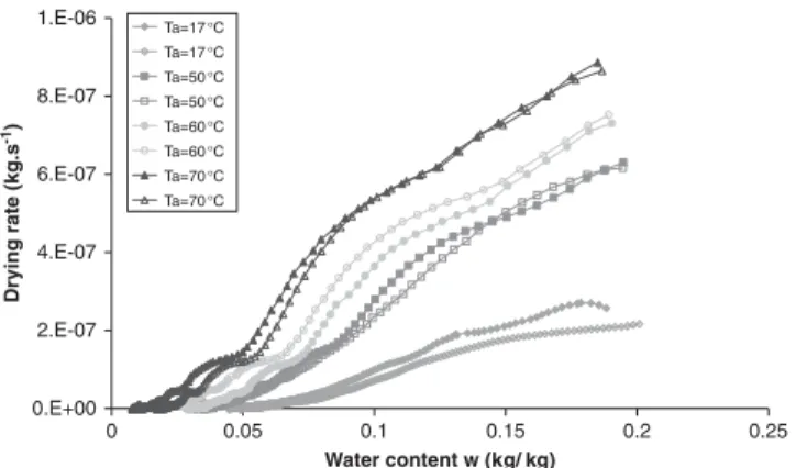
In a second series of tests, different drying temperatures are imposed for air relative humidity of about 1%. Drying curves are shown in Figure 7. The results show the increase in the maximal drying rate with temperature. The duration of the constant drying rate period seems to decrease with temperature. It can be explained by the lower efficiency of the drying process with cold
α = 0.047 -0.026 RH R2 = 0.8819 0 0.01 0.02 0.03 0.04 0.05 0.06 0 β = 16.43 RH + 41.9 R2 = 0.234 0 10 20 30 40 50 60 0.1 0.2 0.3 0.4 0.5 0.6 0 0.1 0.2 0.3 0.4 0.5 0.6 (a) (b)
Figure 6. (a) Mass and (b) heat transfer coefficients according to air relative humidity (air drying temperature Ta=50◦C, air velocity=1m/s).
0.E+00 2.E-07 4.E-07 6.E-07 8.E-07 1.E-06 0 Ta=17°C Ta=17°C Ta=50°C Ta=50°C Ta=60°C Ta=60°C Ta=70°C Ta=70°C 0.05 0.1 0.15 0.2 0.25
Figure 7. Drying curves for different air drying temperatures (air RH≈1%, air velocity=1m/s). surrounding air, comparing with hot surrounding air. The more the drying conditions are severe (hot air), the more the internal transfers of water are the limiting drying mechanism, in comparison to the exchanges into the boundary layer.
Figure 8(a) shows that the mass transfer coefficient does not vary with air drying temperature. In the same way, heat transfer coefficient remains constant with air drying temperature (Figure 8(b)). These results confirm those obtained by Grzegorz and Jacek[15] on kaolin.
Knowing the transfer coefficients, the determination of the water pressure distributions for problems of soils in contact with the ambient conditions becomes possible. Modelling of such drying experiments is interesting in order to validate the vapour and heat transfer expressions between the materials and the surroundings, as proposed in this paper. It can also emphasize the different moisture transport mechanisms.
4. COUPLED 2D FINITE ELEMENT AND FLOW BOUNDARY FINITE ELEMENT FORMULATIONS
In the numerical study, the geomaterials are porous media generally considered as the superposition of several continua [31]: the solid skeleton (grains assembly) and the fluid phases (water, air,
α = -1E-05 Ta + 0.040 0 0.01 0.02 0.03 0.04 0.05 0.06 β = 52.7 - 0.035 Ta 0 10 20 30 40 50 60 70 0 20 40 60 80 0 20 40 60 80 (a) (b)
Figure 8. (a) Mass and (b) heat transfer coefficients according to air drying temperature (air RH≈1%, air velocity=1m/s).
oil, etc.). Based on averaging theories[32, 33], Lewis and Schrefler [34] proposed the governing equations for the full dynamic behaviour of a partially saturated porous medium. Hereafter these equations are restricted for quasi-static problem in unsaturated and non-isothermal conditions, under Richard’s assumptions (constant air pressure). This assumption may be irrelevant in the particular case of low and ultra low permeable porous media.
For this study, incompressible solid grains are assumed. The unknowns of the mechanical, the flow and the thermal problems are, respectively, the displacements ui, the pore water pressure pw (possibly negative in unsaturated case) and the temperature T . In the following developments, the balance equations are written in the current solid configuration denoted #t (updated Lagrangian formulation).
4.1. Balance of momentum
In the mixture balance of momentum equation, the interaction forces between fluid phases and grain skeleton cancels. In a weak form (virtual work principle), this equation reads for any kinematically admissible virtual displacement field u∗
i: % #t& t ijε∗ijd#t= % #t($s (1−'t)+ Sr,wt $tw't)giu∗id#t+ % "t&¯t t iu∗i d"t (6) where ε∗
ij=12((!u∗i/!xtj)+(!u∗j/!xit))is the kinematically admissible virtual strain field, 't is the porosity defined as 't=#v,t/#t where #t is the current volume of a given mass of skeleton and #v,t the corresponding porous volume, $s is the solid grain density, St
r,w is the water relative saturation, $t
wis the water density, gi is the gravity acceleration and "t&is the part of the boundary where tractions¯tt
i are known. The total stress &t
ij is defined as a function of the kinematics. Here we assume first that Bishop’s definition of effective stress holds[35]
&tij=&
&t
ij− Sr,wt ptw(ij (7)
with &&t
4.2. Mass balance equation for the water species
The mass conservation equation of water species is obtained by summing the balance equation of liquid water and water vapour. The water mass balance equation reads in a weak form
% #t " ˙ Mtpw∗−mti!pw∗ !xt i # d#t= % #t Qtp∗wd#t− % "tq ¯qtpw∗d"t (8) where p∗
w is the virtual pore water pressure field, Qt is a sink term and "tq is the part of the boundary where the input water mass per unit area ¯qt is prescribed. Mt and mt
i are, respectively, the mass of the water inside the current configuration of the skeleton #t and the mass flow. They are defined hereafter, respectively, in Equations (9) and (12).
Water mass balance equation (Equation (8)) has to hold for any time t, the virtual quantities in this equation being dependant on the history of boundary conditions and on time t.
The mass flow mt
i is defined by the sum of the advection of the liquid water fi,wt (Darcy’s law for unsaturated cases) and the diffusion of water vapour it
i,v (Fick’s diffusion law). The vapour diffusion follows the formulation proposed by Philip and de Vries [36]. The advective flux of the gaseous phase is neglected because the gas pressure remains constant. The mass flow is thus expressed as follows: mti= fi,wt +ii,vt = −$tw )ktr,w *w "!pt w !xt i +$ t wgi # − D!'t(1− Sr,wt )!$ t v !xt i (9) where ) is the intrinsic permeability, kt
r,wis the water relative permeability, *wis the water dynamic viscosity, D is the molecular diffusion coefficient of the mixture of gaseous air and water vapour, ! the tortuosity and $tvthe vapour density.
The compressible fluid is assumed to respect the following relationship[34]. This predicts an increase of water density as a function of the pore water pressure (defining +was the water bulk modulus) and of the temperature (defining %was the water thermal expansion coefficient):
˙$tw=$tw" ˙p t w +w −%w˙T # (10) Vapour is assumed to be in equilibrium with liquid water and vapour density is given by the following thermodynamic relationship:
$tv=$tv,0hrt (11)
where $t
v,0 is the saturated water vapour density and htr is the relative humidity. The vapour is considered as a perfect gas and the gradient of the water vapour can be separated into two contributions: an isothermal one related to a suction gradient and a thermal one due to a temperature gradient (see[37] for more details about the equations).
If the grains are assumed to be incompressible (which means $sis constant), the time derivative of the water species mass ˙Mt contains two contributions: the liquid water and the water vapour storage variations. The first one is obtained directly by using Equation (10) and mass balance
equation for the solid phase. The second one is deduced from Equation (11). This yields for a unit mixture volume the following:
˙ Mt= $tw !" ˙pt w +w −%w˙T # Sr,wt 't+ ˙Sr,wt 't+ Sr,wt ˙# t #t $ +$tv ! − ˙Sr,wt 't+(1− Sr,wt ) ˙#t #t $ + ˙$tv't(1− Sr,wt ) (12)
4.3. Energy balance equation
Neglecting kinetic energy and pressure energy terms and using the water vapour balance equation in order to evaluate the evaporation rate[37], energy balance equation is written as
% #t " ˙htT∗−tt i!T ∗ !xt i # d#t=% #tF tT∗d#t−% "tq ¯ftT∗d"t (13)
where T∗ is the virtual temperature, ht is the enthalpy of the medium, tt
i is the heat flow, Ft is a volume heat source and ¯ft is the heat flux at the boundary of the materials.
The heat transport is related to three effects: conduction, convection by the fluids and evaporation
tit=−,t!Tt
!xit +(cp,w$ t
wfi,wt +cp,vii,vt )(Tt−T0)+ Lii,vt (14)
with ,t the medium conductivity, cp,w the water specific heat and cp,v the vapour specific heat. The enthalpy of the system is given by the sum of each component’s enthalpy (see [37] for more details):
ht= 'tSr,wt $twcp,w(Tt−T0)+(1−'t)$scp,s(Tt−T0)
+'t(1− Sr,wt )$tvcp,v(Tt−T0)+'t(1− Sr,wt )$tvL (15) with cp,s the solid specific heat.
4.4. Thermal and flow boundaries conditions
The drying process occurs when an initial thermodynamic imbalance exists between the vapour concentration of the surrounding air and the vapour concentration within the sample. Vapour exchanges take place from the materials surface to the surrounding air. In many cases, vapour transfers are modelled by a decrease in the water pressure at the boundary down to the corresponding surrounding suction[8, 16]. This boundary condition relies on the assumption of a quasi-instantaneous equilibrium between the air relative humidity of the atmosphere and the one of the porous medium. This assumption could be too optimistic, because it increases the soil strength due to suction. We assume that a boundary layer at the rock surface exists and vapour transfers take place therein[14]. The water vapour transport is expressed as the difference of the vapour density between the surroundings and the external surface of the samples, multiplied by
a mass transfer coefficient #t, depending on the degree of saturation at the sample boundary S"t r,w [4, 12, 13]:
¯qt=#(Sr,w",t).($",tv −$av) (16)
The drying process occurs in non-isothermal conditions and the heat exchanges between the atmosphere and the material are expressed by Equation (2).
The mass and heat transfer coefficients have been determined from drying experimental results during the constant drying rate period. The set of Equations (2) and (6) to (16) provides a consistent mathematical model of convective drying of capillary-porous media in non-isothermal conditions.
4.5. Thermo-hydro-mechanical finite element formulation
For a given boundary value problem at time t, the equilibrium is not a priori met and some residuals appear, respectively, in the expression of the three field equations (Equations (6), (8) and (13)). In order to solve this non-linear problem, a Newton–Raphson scheme is proposed to find a new solution of displacements, pressures and temperatures field, for which equilibrium is met. The idea is to define a linear auxiliary problem derived from the continuum one (instead of the discretized one as it is more usually done) similar to the work of Borja and Alarcon [38]. This approach gives the same results as standard FEM procedure but make the linearization easier, especially for coupled problem in large strain formulation.
In this paper, linearization of balance equations is not fully developed and we refer to devel-opments in the work of Gerard et al. [4] for a non-saturated porous medium in isothermal conditions. The difference in the linearization procedure comes from the energy balance equation (Equation (13)), which depends on the temperature field.
To reproduce the water vapour and heat flows occurring at the sample surface, we need classical quadrilateral 2D finite elements associated with a new boundary finite element through which the hydric and heat exchanges between the porous medium and the surroundings take place. The special boundary element has been developed in the finite element code Lagamine and is defined by four nodes (Figure 9). The first three nodes are located on the boundary (N1, N2 and N3). They allow a spatial discretization of the water pressure and temperature distribution along the boundary. The fourth node (N4) is introduced to define the relative humidity and the temperature of the surrounding air (as far as they correspond to the d.o.f. of the fourth node). Its geometrical position does not influence the results. Although the atmosphere conditions remain constant during the drying tests, this fourth node will be helpful for the modelling of soil–atmosphere interaction problems. In the following, the finite element formulation of the problem is presented. More details about the numerical description of the four nodes boundary finite element can be found in Gerard
et al.[4].
Following the linearization procedure of the non-linear problem (see[4, 39] for the details), the linear auxiliary problem is found and the three corresponding equations are rewritten in a matricial form, in order to define the local element stiffness matrix
% #t[U
∗,t
(x,y)]T[Et][dU(tx,y)]d# t−%
"tq
[U(∗,tx,y)]T[Ft][dU(tx,y)]d" t
q= Rt+Vt+Wt (17)
where Rt, Vt and Wt are, respectively, the residuals of the mechanical, the flow and the thermal problems,[dUt
Figure 9. Two-dimensional finite element and boundary element. corresponding virtual quantities:
[dUt (x,y)]T≡ &!dut 1 !x1t !dut 1 !x2t !dut 2 !x1t !dut 2 !x2t dut1dut2!dptw !x1t !dpt w !x2t d ptw!dTt !x1t !dTt !x2t dTt ' (18) In Equation (17), the first left-hand term is computed by a 2D coupled finite element and the second left-hand term is evaluated by the 1D boundary finite element. The finite element spatial discretization is introduced in Equation (17) using the transformation matrices[Tt] and [B] for the 2D finite element (and, respectively,[St] and [C] for the boundary finite element), with connect [dUt
(x,y)] to the nodal variables [dUNodet ]. Integration of the two left-hand terms of Equation (17) on a finite element yields:
[Unode2D,∗]T % 1 −1 % 1 −1[B] T[Tt]T[Et][Tt][B]det Jtd-d.[dU2D,t Node] −[UnodeBE,∗]T
% 1 −1[C]
T[St]T[Ft][St][C]det Ntd/[dUBE,t Node] ≡[Unode2D,∗]T[k2D,t][dUNodet ]−[UnodeBE,∗]T[kBE,t][dUNodeBE,t]
(19)
where[k2D,t] and [kBE,t] are the local element stiffness matrices, respectively, of the 2D finite element and of the boundary finite element, Jt is the Jacobian matrix of the mapping from (-,.) to (x, y) for the 2D finite element (and Nt is the Jacobian matrix of the mapping from (/) to (x, y) for the boundary finite element).
[Et] and [F!1] are (12×12) matrices that contain all the terms of equations coming from linearization, respectively, for 2D finite element and boundary finite element:
[Et] = KMM2D,t(6 ×6) K 2D,t WM(6×3) K 2D,t TM(6×3) KMW2D,t(3 ×6) K 2D,t WW(3×3) K 2D,t TW(3×3) KMT2D,t(3 ×6) K 2D,t WT(3×3) K 2D,t TT(3×3) (20)
[Ft] = 0(6×6) 0(6×3) 0(3×3) KMWBE!1 (3×6) K BE WW!1 (3×3) K BE TW!1 (3×3) KMTBE!1 (3x3) K BE WT!1 (3×3) K BE TT!1 (3×3) (21)
Matrix[Et] is composed by the classical stiffness matrices for the mechanical, the flow and the thermal problems with 2D finite element. Their formulations can be found in Collin et al.[37].
KBE
MW, KWWBE and KTWBE contain all the terms appearing due to the dependence of the total boundary flow ¯qt with displacement, hydraulic and temperature fields. KBE
MT, KWTBE and KTTBE contain all the terms appearing due to the dependence of the boundary heat ¯ft with displacement, hydraulic and temperature fields. These stiffness matrices of the boundary element are detailed hereafter.
KMWBE,t(3 ×6)= 0 0 0 0 0 0 0 0 0 0 0 0 qt 0 0 qt 0 0 ; KWWBE,t(3×3)= 0 0 0 0 0 0 0 0 Z KTWBE,t(3 ×3)= 0 0 0 0 0 0 0 0 X (22) KMTBE,t(3 ×6)= 0 0 0 0 0 0 0 0 0 0 0 0 ft 0 0 ft 0 0 ; KWTBE,t(3×3)= 0 0 0 0 0 0 0 0 L· Z KTTBE,t(3 ×3)= 0 0 0 0 0 0 0 0 %+ L · X (23) Z= #(S",t r,w) Mvh",tr $",tv,0 RT",t . 1 $",tw −(pw",t− p",tg )+w $w,0(pw",t)2 / +!#",t !Sr,w",t !Sr,w",t !p",tw ($",tv −$av) (24) X= #(S",t r,w)hr",t ! !$",tv,0 !T",t− Mv$",tv,0(pw",t− p",tg ) R(T",t)2$",t w +Mv$ ",t v,0(pw",t− p",tg ) R(T",t)3$ w,0%w $ (25)
5. NUMERICAL MODELLING OF CONVECTIVE DRYING TESTS ON SILTS
5.1. Boundary value problem
The main aim of the work is to compare the convective drying experimental data with the simulation results. 2D-axisymetric modellings of cylindrical samples are performed. The porous medium is assumed rigid. Gas pressure is assumed constant and equal to the atmospheric pressure.
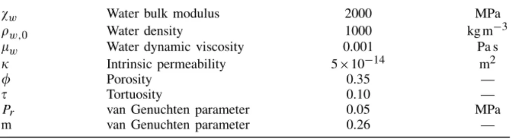
Figure 10. Boundary value problem of drying experiment. Table I. Parameters of the flow model.
+w Water bulk modulus 2000 MPa
$w,0 Water density 1000 kg m−3
*w Water dynamic viscosity 0.001 Pa s
) Intrinsic permeability 5×10⁻¹⁴ m2
' Porosity 0.35 —
! Tortuosity 0.10 —
Pr van Genuchten parameter 0.05 MPa
m van Genuchten parameter 0.26 —
The geometry of the problem is presented on Figure 10. The samples are initially saturated and their initial temperature is the ambient temperature (=17◦C). The temperature and the relative humidity of the atmosphere are imposed at the corresponding node. Heat and flow transfers with the exterior are described by Equations (2) and (16). Mass and heat transfer coefficients computed from the drying experiments in Section 3 are used in the boundary condition expressions.
5.2. Hydraulic and thermal properties
The relationships describing the hydraulic and the thermal properties are developed in the Sections 4.2 and 4.3. The parameters used in the modelling of the drying tests have been determined by Masekanya[27] (Table I). The parameters used for the retention curve are those defined in Section 3.2 in the van Genuchten relationship. The water relative permeability function proposed by van Genuchten[28] is adopted:
kr,w=0Sr,w[1−(1− Sr,w1/m)m]2 (26)
For the modelling of the thermal problem, the following parameters are used (Table II). It is known that the thermal conductivity of soils depends on temperature and saturation, but a constant thermal conductivity is used in the modelling, due to a lack of experimental data on Awans silt.
Table II. Parameters of the thermal model.
%w Water thermal expansion coefficient 3×10⁻⁴ K−1
cp,w Water specific heat 4180 Jkg−1K−1
cp,s Solid specific heat 879 Jkg−1K−1
cp,v Vapour specific heat 1000 Jkg−1K−1
" Thermal conductivity 1.3 W m−1K−1 -1.E-07 0.E+00 1.E-07 2.E-07 3.E-07 4.E-07 5.E-07 0.00 Experiment Simulation 15 20 25 30 35 40 45 50 55 0 0.05 0.10 0.15 0.20 0.25 0.5 1 1.5 (a) (b)
Figure 11. (a) Drying curves—Comparison between experimental and numerical results. (b) Time evolution of temperature at the silt surface. Numerical results of drying tests
with air RH=30% and Ta=50◦C.
5.3. Influence of flow boundary condition on the modelling results
A drying test performed with an air relative humidity of 30% and a temperature of 50◦C is first modelled. The advantage of this experiment is that the air relative humidity is situated in a range of values where the retention behaviour has been experimentally determined (Figure 4). In this first simulation, mass transfer coefficient is assumed independent of the degree of saturation at the boundary of the sample (Equation (16)). In this way we assume that the boundary layer, where the vapour transfers occur, remains saturated during the drying. The value of the mass transfer coefficient, as well as the heat transfer coefficient, is those determined from experimental results during the constant drying rate period.
The drying curve obtained with these parameters is presented in Figure 7(a). The constant drying rate period obtained with the modelling is more pronounced than the one observed experimentally. Temporal evolution of temperature at the sample boundary is plotted in Figure 11(b). A clear stabilization of the temperature at the wet bulb temperature can be observed, corresponding to the constant drying rate period. At the end of the drying, the temperature reaches the temperature of the surrounding medium.
Assumption of non-isothermal conditions is necessary to reproduce such drying behaviour. Initial vapour density at the boundary of the sample is indeed lower than vapour density of the surroundings. Initially, moisture transport occurs initially from the ambient medium to the silt, which is thus moistened. Nevertheless, during the preheating period, temperature at the boundary of the sample quickly increases, accruing its vapour density. Evaporation flow becomes positive and the material is dried.
-1.E-07 0.E+00 1.E-07 2.E-07 3.E-07 4.E-07 5.E-07 0.00 Experiment Simulation 15 20 25 30 35 40 45 50 55 0 0.05 0.10 0.15 0.20 0.25 0.5 1 1.5 (a) (b)
Figure 12. (a) Drying curves with new flow boundary condition—Comparison between experimental and numerical results. (b) Time evolution of temperature at the silt surface. Numerical results of drying test
with air RH=30% and Ta=50◦C.
The overestimation of the drying rate should be reduced (Figure 11(a)). It can be imagined that the boundary layer where the vapour exchanges take place does not remain saturated during the falling drying rate period, due to the slowness of moisture transport compared with the capacity of evaporation of the boundary layer. If the mass transfer coefficient is influenced by the desaturation of the boundary layer, the vapour transport at the sample surface can be modified. Assuming a linear relation between the mass transfer coefficient and the degree of saturation at the boundary surface, Equation (16) becomes
¯q =#0· Sr,w" ·($"v−$av) (27)
with #0 the saturated vapour transfer coefficient, corresponding to the one determined during the constant drying rate period.
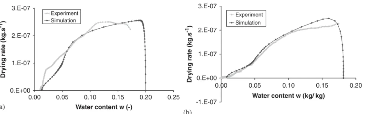
With this new flow boundary condition, numerical results present good agreement with exper-imental measurements, as shown in Figure 12(a) for a drying test performed with an air relative humidity of 30% and a drying temperature of 50◦C. Owing to the desaturation of the boundary layer, the constant drying rate period is reduced and the falling rate period begins earlier. Moreover, the temperature at the boundary of the sample does not remain constant at the wet bulb temperature (Figure 12(b)). The decrease of the vapour transfer coefficient with desaturation reduces indeed the moisture transport to the boundary. The heat provided by the atmosphere is sufficient enough for the quantity of water evaporating at the boundary layer and, as a consequence, temperature at the boundary increases.
Other drying tests can be modelled satisfactorily with flow boundary condition expressed in Equation (27), as shown in Figure 13. We recall that a filter operation on experimental data induces the loss of initial and final information.
6. MOISTURE TRANSPORT MECHANISMS
The purpose of this section is the study of the moisture transport during the drying of highly permeable materials: it is mainly achieved by water evaporation within the sample followed by vapour diffusion towards the ambient medium (i.e. 1+2 in Figure 14) or by the liquid water transport to the boundary of the sample where it evaporates (i.e. 1&+2& in Figure 14)[19]?
0.E+00 1.E-07 2.E-07 3.E-07 0.00 Water content w (-) Dr ying rate (kg.s -1) Experiment Simulation -1.E-07 0.E+00 1.E-07 2.E-07 3.E-07 Water content w (kg/ kg) Dr ying rate (kg.s -1) Experiment Simulation 0.05 0.10 0.15 0.20 0.00 0.05 0.10 0.15 0.20 0.25 (a) (b)
Figure 13. Drying curves with new flow boundary condition—Comparison between experimental and numerical results (a) RH=50%, Ta=50◦C and (b) RH=1%, Ta=17◦C.
Figure 14. Schematic representation of two extreme moisture transport mechanisms[19].
Coussy [10] explained that, when the intrinsic permeability ) is lower than 10−19m2, the liquid transport inside the porous space and evaporation at the boundary are the only dominant mechanisms of moisture removal. Indeed the combined and opposite diffusion of dry air and water vapour makes the molar concentration rapidly uniform and, thus, later renders the diffusion process inactive as a motor of the drying process[19]. Silts clearly do not lie in this range of permeability and the moisture transport mechanism should be studied.
The mechanism of moisture transport is different for materials with high permeability. Figure 15 presents the temporal evolution of water and vapour flows at the sample surface (in the middle of the height of the sample) obtained from numerical modelling of drying experiments on silt. We show that moisture is first mainly removed by liquid water advection (Darcy’s law). When the desaturation of the boundary begins, Darcy’s water flow decreases and vapour diffusion becomes predominant at the sample surface.
The profiles of water and vapour flows along a horizontal section situated at the middle of the height of the sample (Figure 16) show that initially the transport of humidity within the whole sample corresponds in its major part to the internal transport of liquid, followed by evaporation at the sample surface. The limiting step is thus the exchanges in the boundary layer. Vapour density is uniform in the sample (Figure 17). Owing to temperature increase, intense evaporation occurs
0.0E+00 5.0E-05 1.0E-04 1.5E-04 2.0E-04 2.5E-04 0 Time (h) Flo w (kg.m -2.s -1)
External vapour flow Liquid water advective flow Vapour diffusion
0.5 1 1.5 2 2.5
Figure 15. Temporal evolution of water and vapour flows at the sample surface (in the first element at the middle of the height)—Drying modelling with RH=30%, Ta=50◦C.
0.E+00 1.E-05 2.E-05 3.E-05 4.E-05 5.E-05 6.E-05 7.E-05 8.E-05 0.003 0.006 0.009 0 r (m) Flo w (kg.m -2.s -1) 1h05 1h05 1h10 1h10 1h20 1h20 1h50 1h50 Water advection Vapour diffusion
Figure 16. Water and vapour flows profiles along horizontal section situated at the middle of the height of the sample—Drying modelling with RH=30%, Ta=50◦C.
at the sample boundary and desaturation of silts begins. Water advection decreases and vapour density gradient appears in the desaturated zone. A receding front is created and moves to the heart of the sample. The limiting step becomes the internal liquid transport, as the relative permeability is decreasing. The extent of the desaturated zone increases with time. After 2:30 of drying, the vapour distribution becomes again uniform into the sample and the vapour diffusion flows decrease with time (Figures 15, 16 and 17).
Modelling of silts drying emphasizes the influence of vapour diffusion, which was negligible with weakly permeable materials. Indeed high permeability decreases the characteristic time for advective transport for liquid water, as defined by Coussy [10]. It becomes the same order of magnitude as the characteristic time for diffusion. The two transport phenomena thus play a role during the drying experiments.
0 0.1 0.2 0.3 0.4 0.5 0.6 0.7 0.8 0.9 1 0 r (m) Relative humidity (-) 2h 30min 1h30 2h15 2h30 1h 3h30 0.003 0.006 0.009
Figure 17. Relative humidity profiles along horizontal section situated at the middle of the height of the sample—Drying modelling with HR=30%, Ta=50◦C.
7. CONCLUSIONS AND PERSPECTIVES
When geomaterials are submitted to interactions with the atmosphere, the correct modelling of the coupled vapour and heat exchanges occurring at the surface is needed in order to determine the capillary pressure distributions into the porous medium. Flow and heat boundary conditions reproducing the exchanges occurring at soil surface are therefore needed. For these reasons, convective drying experiments have been performed on samples of Awans silt under different drying conditions (air temperature and relative humidity). The Awans silt is an upper soil from Belgium and is thus representative of the geological layers where the problems of interaction with the ambient atmosphere (as slope stability problems or soils submitted to drought periods) take place. Assuming that the exchanges take place in a boundary layer, mass and heat transfer coefficients can be determined through the drying experiments on initially saturated samples. The results show that mass transfer coefficient remains constant with drying temperature and decreases with air relative humidity. A tendency for heat transfer coefficient with drying temperature or air relative humidity is more difficult to define.
Modellings of the drying tests under non-isothermal conditions have been performed. Assuming the existence of a boundary layer where the exchanges take place allows a good reproduction of the kinetic of drying observed during the experiments. We have showed the relevance of our model: the dependence of the transfer coefficients with the desaturation of the boundary layer. In this way, the overestimation of the drying rate is avoided, which is not the case when the capillary pressure at the boundary is numerically imposed to the ambient suction. Such modellings allow the validation of the proposed formulation for the coupled flow and heat exchanges occurring at soils surface in interaction with the atmosphere. Numerical results also improve the understanding of the moisture transfer mechanisms into the porous medium and the exchanges with the ambient atmosphere. It is showed that in a first time, liquid water advection is the main mechanism of water transport into the sample. Then vapour diffusion becomes predominant and it corresponds with the decrease of relative humidities into the sample.
The experimental determination of the transfer coefficients assumes a saturated initial state and a boundary temperature equal to the wet bulb temperature during the constant flow period. For partially saturated initial state, the preceding assumptions have to be discussed. Knowing the initial saturation, the mass transfer coefficient #0could be computed at the maximal experimental drying flow from Equation (27). In this latter case, additional assumptions are necessary: at the maximum drying flow, the boundary saturation is not far from the initial one and the boundary temperature is supposed to be equal to the wet bulb temperature. These assumptions are all the more realistic so the initial suction is low.
Such flow and heat boundary conditions can be used in numerical study of soil–atmosphere interaction problems in order to deduce the capillary pressure distributions into the geomaterials. Nevertheless, in the context of ventilated cavities for radioactive waste disposals, this model should be extended. Indeed, in weakly permeable geological layers, gas overpressures can be generated, which modify the kinetic and the mechanisms of the desaturation of the rock mass. Gas overpres-sures can no more be disregarded and has to be taken into account[10, 19]. Moreover cracking or microcracking could also be observed during the desaturation, which influences probably the parameters controlling the vapour exchanges (permeability, transfer coefficients. . .).
ACKNOWLEDGEMENTS
The authors thank the FRS-FNRS and the European project TIMODAZ for their financial support. TIMODAZ is cofunded by the European Commission (EC) as part of the sixth Euratom research and training Framework Programme (FP6) on nuclear energy (2002–2006).
REFERENCES
1. Delay J, Vinsot A, Krieguer JM, Rebours H, Armand G. Making of the underground scientific experimental programme at the Meuse/Haute-Marne underground research laboratory, North Eastern France. Physics and
Chemistry of the Earth2007; 32:2–18.
2. Mayor JC, Velasco M, Garc´ıa-Sineriz JL. Ventilation experiment in the Mont Terri underground laboratory.
Physics and Chemistry of the Earth2007; 32:616–628.
3. Ghezzehei TA, Trautz RC, Finsterle S, Cook PJ, Ahlers CF. Modeling coupled evaporation and seepage in ventilated cavities. Vadose Zone Journal 2004; 3:806–818.
4. Gerard P, Charlier R, Chambon R, Collin F. Influence of evaporation and seepage on the convergence of a ventilated cavity. Water Resources Research 2008; 44:W00C02. DOI: 10.1029/2007WR006500.
5. Homand F, Giraud A, Escoffier S, Koriche A, Hoxha D. Permeability determination of a deep argillite in saturated and partially saturated conditions. International Journal of Heat and Mass Transfer 2004; 47:3517–3531. 6. Giraud A, Giot R, Homand F, Koriche A. Permeability identification of a weakly permeable partially saturated
porous rock. Transport in Porous Media 2007; 69:259–280.
7. Baroghel-Bouny V, Mainguy M, Coussy, O. Isothermal drying process in weakly permeable cementitious materials—assessment of water permeability. In Material Science of Concrete, Special Volume: Ion and Mass
Transport in Cement Based Materials, Hooton RD, Thomas MDA, Marchand J, Beaudoin JJ (eds). American Ceramic Society: Westerville, OH, 2001; 59–80.
8. Giraud A, Giot R, Homand F. Poromechanical modelling and inverse approach of drying tests on weakly permeable porous rocks. Transport in Porous Media 2009; 76(1):45–66.
9. Baggio P, Bonacina C, Schrefler BA. Some considerations on modeling heat and mass transfer in porous media.
Transport in Porous Media1997; 28:233–251. 10. Coussy O. Poromechanics. Wiley: London, 2004.
11. Olivella S, Gens A. Vapour transport in low permeability unsaturated soils with capillary effects. Transport in
Porous Media2000; 40:219–241.
13. Coumans WJ. Models for drying kinetics based on drying curves of slabs. Chemical Engineering and Processing 2000; 39(1):53–68.
14. Kowalski SJ. Thermomechanics of Drying Processes. Lecture Notes in Applied and Computational Mechanics. Springer: Berlin, 2003.
15. Grzegorz M, Jacek B. Non-linear heat and mass transfer during convective drying of kaolin cylinder under non-steady conditions. Transport in Porous Media 2007; 66:121–134.
16. Hoxha D, Giraud A, Blaisonneau A, Homand F, Chavant C. Poroplastic modelling of the excavation and ventilation of a deep cavity. International Journal of Numerical and Analytical Methods in Geomechanics 2004; 28:339–364.
17. Delage P, Howat MD, Cui YJ. The relationship between suction and swelling properties in a heavily compacted unsaturated clay. Engineering Geology 1998; 50:31–48.
18. Coussy O, Eymard R, Lassabat`ere T. Constitutive modelling of unsaturated drying deformable materials. Journal
of Engineering Mechanics(ASCE) 1998; 124(6):658–667.
19. Mainguy M, Coussy O, Baroghel-Bouny V. Role of air pressure in drying of weakly permeable materials. Journal
of Engineering Mechanics(ASCE) 2001; 127(6):582–592.
20. L´eonard A, Blacher S, Marchot P, Crine M. Use of X-ray microtomography to follow the convective heat drying of wastewater sludges. Drying Technology 2002; 20(4–5):1053–1069.
21. Nadeau J-P, Puiggali JR. S´echage—Des Processus Physiques Aux proc´ed´es Industriels. Technique et Documentation—Lavoisier: Paris, 1995.
22. Geankoplis CJ. Transport Processes and Unit Operations. Prentice-Hall: Englewood Cliffs, NJ, 1993.
23. L´eonard A, Blacher S, Marchot P, Pirard J-P, Crine M. Convective drying of wastewater sludges: influence of air temperature, superficial velocity and humidity on the kinetics. Drying Technology 2005; 23(8):1667–1679. 24. Dracos Th. Hydrologie, Eine Einf¨uhrung f¨ur Ingenieure. Springer Wien: New York, 1980.
25. Ketelaars AAJ. Drying deformable media—Kinetics, shrinkage and stresses. Ph.D. Thesis, Technische Universiteit Eindhoven, 1992.
26. Anagnostou G. Seepage flow around tunnels in swelling rock. International Journal for Numerical and Analytical
Methods in Geomechanics1995; 19:705–724.
27. Masekanya J-P. Stabilit´e des pentes et saturation partielle—etude exp´erimentale et mod´elisation num´erique. Ph.D.
Thesis, Universit´e de Li`ege, 2008.
28. van Genuchten MTh. A closed-form equation for predicting the hydraulic conductivity of unsaturated soils. Soil
Science Society of America Journal1980; 44:892–898.
29. Nicolas J, Andr´e P, Rivez JF, Debbaut V. Thermal conductivity measurements in soil using an instrument based on the cylindrical probe method. Review of Scientific Instruments 1993; 64(3):774–780.
30. L´eonard A. Etude du s´echage convectif de boues de station d’´epuration—suivi de la texture par microtomograhie `a rayons X. Ph.D. Thesis, Universit´e de Li`ege, 2003.
31. Coussy O. Mechanics of Porous Continua. Wiley: London, 1995.
32. Hassanizadeh M, Gray W. General conservation equations for multi-phase systems: 1. Average procedure.
Advances in Water Resources1979; 2:131–144.
33. Hassanizadeh M, Gray W. General conservation equations for multi-phase systems: 2. Mass, momenta, energy, and entropy equations. Advances in Water Resources 1979; 2:191–208.
34. Lewis RW, Schrefler BA. The Finite Element Method in the Static and Dynamic Deformation and Consolidation
of Porous Media. Wiley: New York, 2000.
35. Nuth M, Laloui L. Effective stress concept in unsaturated soils: clarification and validation of a unified framework.
International Journal for Numerical and Analytical Method in Geomechanics 2008; 32:771–801.
36. Philip JR, de Vries DA. Moisture movement in porous materials under temperature gradients. Eos Transactions
American Geophysical Union1957; 38(2):222–232.
37. Collin F, Li XL, Radu JP, Charlier R. Thermo-hydro-mechanical coupling in clay barriers. Engineering Geology 2002; 64:179–193.
38. Borja R, Alarcon E. A mathematical framework for finite strain elastoplastic consolidation Part 1: balance law, variational formulation and linearization. Computers Methods in Applied Mechanics and Engineering 1995; 122:765–781.
39. Collin F, Chambon R, Charlier R. A finite element method for poro mechanical modelling of geotechnical problems using local second gradient models. International Journal for Numerical Methods in Engineering 2006; 65(11):1749–1772.