Transversal assessment of new intermodal strategies : deliverable D 7.1, synopsis

Deliverable D 7.1

Synopsis

31/07/2018

BRAIN-TRAINS

Transversal assessment of new

intermodal strategies

Frank Troch, Thierry Vanelslander, Christa Sys, Koen Verhoest, Christine Tawfik, Sabine Limbourg, Angel Merchan, Angélique Léonard

BELGIAN RESEARCH ACTION THROUGH

INTERDISCIPLINARY NETWORKS

CONTENTS

CONTENTS ... 2

INTRODUCTION ... 4

1. User guide of the methodology of WP2: optimal corridor and hub development ... 6

1.1. Introduction ... 6

1.2. Model 1: location/allocation model ... 6

1.2.1. General description ... 6

1.2.2. Input values: parameters ... 7

1.2.3. Output values: variables ... 8

1.2.4. What can the model bring in terms of transport policy? How can the resulting indicators be interesting? ... 8

1.2.5. Limitations ... 9

1.3. Model 2: Service Network Design Model ... 10

1.3.1. General description ... 10

1.3.2. Scenario Parameters and outputs ... 10

1.3.3. Additional hypotheses ... 11

1.3.4. What can the model bring in terms of transport policy? How can the resulting indicators be interesting? ... 11

1.3.5. Limitations ... 11

2. User guide of the methodology of WP3: economic impact ... 13

2.1. Introduction ... 13

2.2. Model 1: added value and employment micro-analysis ... 13

2.2.1. General description ... 13

2.2.2. Output values: three indicators ... 14

2.2.3. Input values: data collection ... 14

2.2.4. Limitations ... 17

2.3. Model 2: added value and employment sector-analysis (input-output) ... 17

2.3.1. General description ... 17

2.3.2. First step: collecting supplier and customer data ... 18

2.3.3. Second step: adapting the supply and demand table ... 19

2.3.4. Third step: creating the new input-output table... 20

2.3.5. Fourth step: calculating the Leontief multiplier ... 20

3. User guide of the methodology of WP4: sustainability impact ... 22

3.1. Introduction ... 22

3.2. Methodology ... 22

3.2.1. Goal and scope definition ... 23

3.2.2. Life Cycle inventory ... 23

3.2.3. Life Cycle inventory Impact assessment ... 27

3.2.4. Life cycle interpretation ... 27

4. User guide of the methodology of WP5: market regulation ... 28

4.1. Introduction ... 28

4.2. Methodology ... 28

4.3. Indicators for a static approach of competition ... 28

4.3.1. The Herfindahl – Hirschman index (HHI) ... 29

4.3.2. The Concentration Ratio (CR): ... 29

4.3.3. The Equivalent Number (EN): ... 29

4.4. Indicators for a dynamic approach of competition ... 30

4.4.1. The Persistence Of Profit (POP): ... 30

4.4.2. The Capital cost/Labor cost ratio (C/L ratio): ... 30

5. User guide of the methodology of WP6: governance and organization... 32

5.1. Self-assessment instrument regarding policy integration ... 32

5.2. Self-assessment instrument regarding administrative integration ... 38

5.3. Self-assessment instrument regarding institutional changes ... 42

INTRODUCTION

Over the period 2014 – 2018, the BRAIN-TRAINS project analysed rail freight developments within an intermodal context in Belgium (https://www.brain-trains.be). The main goal of the project is to develop a blue print, including the detailed criteria and conditions for developing an innovative intermodal network in and through Belgium, as part of the Trans-European Transport Network (TEN-T) in order to meet different market, societal and policy-making challenges. The project developed an operational framework in which effective rail freight transport and intermodal transport can be successfully established in Belgium, with attention to beneficial participation and commitment of all different stakeholders.

This interdisciplinary analysis is built around seven Work Packages (WP’s), focussing on five different main topics, as shown in Figure 1.

FIGURE 1. STRUCTURE OF THE BRAIN-TRAINS PROJECT

The BRAIN-TRAINS project started with an analysis of the rail freight market in WP 1. In order to provide the correct context for the rest of the project, a SWOT analysis has been performed in Deliverable 1.1 – 1.2. From this analysis, three plausible scenarios for rail freight transport development within an intermodal context have been explored in deliverable 1.3. This best-, medium- and worst-case scenario, together with the SWOT matrix and the SWOT analysis, served as input parameters for the quantification methodologies of the five different topics in WPs 2 to 6.

Each WP adapted or developed a topic-specific methodology, in order to quantify the impact of rail freight transport development and intermodal transport, on the observed indicators. As such, tools are provided for users of rail freight transport or government parties, to define strategies for rail freight transport development based on quantification of possible effects.

The output of these WPs are used in WP 7, to create a synthesis of the developed methodologies in the current deliverable 7.1. The final deliverable 7.2 formulates some ultimate recommendations and provides more insight in possible linkages between the WPs. The current deliverable 7.1 will be structured according to the standard work package division, as presented in Figure 1. For each work package (2 to 6), a summary of the observed indicators and a synopsis of the developed methodology is presented. As such, this obtained knowledge can be used in future research, or when updates of the performed analysis on future trends and developments are desired. As such, this deliverable 7.1 can be considered as a user guide to the methodology developed by the different work packages.

In the next deliverable 7.2, possible linkages and some final recommendations will be made, based on the outcome of the used methodologies.

1. User guide of the methodology of WP2: optimal corridor and hub

development

1.1. Introduction

The objective of this section of deliverable 7.1 is to develop a user guide of the tools developed by Work Package 2 – WP2 (operational issues).

As a reminder, WP 2 aims at providing tools from the operations research domain, in order to highlight how effective intermodal rail transport is in Belgium. The objective of this package is also to give more insight on the decision-making process of the different stakeholders in the intermodal chain. The methods are based on the area of expertise of optimization, which aims at translating a managerial problem into a mathematical model that should be optimized. The main components of the methodology consist of:

1) Identifying the managerial problem;

2) Modelling the problem using mathematical programming; 3) Computing the solutions;

4) Translating the scenarios.

As two different kinds of models have been developed and applied in the framework of the BRAIN-TRAINS project, this user guide is divided into two sections related to the two models developed: (i) intermodal location-allocation model and (ii) service network design.

1.2. Model 1: location/allocation model

1.2.1. General description

The first model that is developed focuses on the strategic horizon level. It is part of the category of models related to intermodal network design. Figure 2 shows the simplified scheme of how the model works.

FIGURE 2 : SIMPLIFIED SCHEME OF THE LOCATION-ALLOCATION MODEL

The definition of the considered scenario leads to the identification of the values of the fixed parameters (= input of the model) to be introduced in the model. After the run of the model, the optimal values of the variables (= output of the model) under study are identified. By modifying the initial values of the parameters (depending on the specific considered scenario) and by re-running the model, new results in terms of variables can be obtained. This allows analyzing of the impacts of the application of a particular policy.

The general formulation of the model is a location-allocation model. This means that the main objective of the mathematical model is to determine the optimal location of the intermodal terminals within a specific geographical region. Moreover, the model allows assessing the flow distribution between the direct and intermodal transport. An intermodal path is constituted by a pre-haulage of the goods by road, a long-haul travel by rail or inland waterways (IWW) and a post-haulage by road. The allocation of

Scenario definition Input (parameters) Run of the model Output (variables) Results in terms of policy

flows of goods is therefore split into three transport possibilities: direct road transport, intermodal rail transport and intermodal IWW transport. Since the BRAIN-TRAINS study aims at providing knowledge on the real case study of Belgium, the location-allocation model has been transformed into an allocation model by taking into account the already existing terminals in the zone. This means that the terminal configuration is therefore a fixed parameter and that it does not have to be determined

1.2.2. Input values: parameters

The input values of the model are of six main types, namely related to:  Operational costs

 Climate change (CO2 emissions, CO2 equivalent emissions)

 Air pollution (air pollution external costs, photochemical ozone formation, particulate matter)

 Demand (origin-destination matrix)  Policy (taxes)

 Terminal locations

The input values of the model are the following ones:  Operational costs – Road long-haul  Operational costs – Road short-haul  Operational costs – Rail

 Operational costs – IWW  Transhipment operational costs  CO2 emissions – Road

 CO2 emissions – Rail (electric)

 CO2 emissions – Rail (diesel)

 CO2 emissions – IWW

 Transhipment CO2 emission

 Air pollution external costs – Road long-haul  Air pollution external costs – Road short-haul  Air pollution external costs – rail

 Air pollution external costs - IWW  Transhipment air pollution external cost

 CO2 equivalent emissions – Road (Belgian values of WP4)

 CO2 equivalent emissions – Rail (Belgian values of WP4)

 CO2 equivalent emissions – IWW (Belgian values of WP4)

 Particulate matter emissions – Road (Belgian values of WP4)  Particulate matter emissions – Rail (Belgian values of WP4)  Particulate matter emissions – IWW (Belgian values of WP4)  Transhipment particulate matter emissions (Belgian values of WP4)  Photochemical ozone formation emissions – Road (Belgian values of WP4)  Photochemical ozone formation emissions – Rail (Belgian values of WP4)  Photochemical ozone formation emissions – IWW (Belgian values of WP4)  Transhipment Photochemical ozone formation emissions (Belgian values of

WP4)

 Demand of transport  Road taxes

The input values aim at evaluating the impact of different policies on the final modal split between direct road, intermodal rail and intermodal IWW transport.

The operational cost values are used as the objective function in order to identify the effect on modal split of a policy which focuses on the optimization of economic goals.

The CO2 emission and CO2 equivalent emission values are used as the objective function in order to

determine the effect on modal split of a policy which focuses on the optimization of climate change goals.

The air pollution external cost, photochemical ozone formation, and particulate matter values are used as the objective function in order to determine the effect on modal split of a policy which focuses on the optimization of air pollution quality goals.

1.2.3. Output values: variables

The output values of the model are the following ones:  Modal split

 Total costs

 Total CO2 emissions

 Total air pollution external costs  Total CO2 equivalent emissions

 Total particulate matter emissions

 Total photochemical ozone formation emissions

1.2.4. What can the model bring in terms of transport policy? How can the resulting

indicators be interesting?

The proposed model generally allows assessing the effects of scenarios on the modal split. The main resulting indicator is therefore the market share attributed to each mode of transport between direct road, intermodal rail and intermodal IWW transport. The following list of examples highlights the practical usefulness of the model in terms of the policies that can be evaluated.

 Evaluation of the impact on the modal split of economic objectives  Evaluation of the impact on the modal split of environmental objectives  Evaluation of the impact on the modal split of different tax levels  Evaluation of the impact on the modal split of different subsidy levels  Evaluation of the impact on the modal split of additional terminals  Evaluation of the impact on the modal split of fewer terminals  Evaluation of the impact on the modal split of a demand variation

 Evaluation of the impact on the modal split of a policy focusing on the internalization of external costs

1.2.5. Limitations

Some limitations of the model relate to the data used in order to evaluate the effects of the scenarios on case studies. Indeed, the origin-destination matrix data are quite old (last extrapolation of the Worldnet 2005 matrix for the year 2010) and it is possible that the structure of flow exchanges has been modified since then. An update of the data could lead to other flow distribution in the case in which economies of scale of intermodal transport would be taken into account. Moreover, the value attributed to the externalities of transport may also evolve. Indeed, depending on the methodology used to value them, and based on continuously updated evaluation of the negative effects of transport, externalities of transport could vary in a quite large range in the future. This situation also influences the results in terms of modal split. Nevertheless, the developed model is still valid in case of data variations. It only needs to be adjusted to the adapted values, in order to identify the impact of demand, costs or externalities variations on the flow distribution between direct road and intermodal rail or IWW transport. A simple re-run of the model with the updated values is sufficient to obtain the new resulting modal split.

For computational reasons, economies of scale of intermodal transport have not been modeled in the present research. This means that the allocation of flows depends on the distance and cost factors which are linear with the distance traveled. However, modeling intermodal economies of scale makes sense since it may highlight how intermodal transport can be more profitable (or not), depending on the level of flows that are consolidated (see Mostert et al., 2017 for an illustration of the differences with and without the modeling of economies of scale). This inclusion of economies of scale is however more difficult to solve because it requires the use of non-linear functions.

The model developed in this research allows evaluating the impact on modal split between road, intermodal rail and intermodal IWW transport of a single policy (either economic, or environmental, or with the introduction of road taxes under economic optimization). However, even if the cost attribute remains one of the main drivers for the choice of a transportation mode, other elements such as time or transport reliability may be relevant. It is possible to introduce these specific characteristics by replacing the current all-or-nothing model by a modal choice model, in which all the flows between a specific origin-destination pair would not necessary be transported by the same mode of transport. Moreover, the balance between environmental and economic objectives could also be evaluated using a bi-objective formulation (see Mostert et al., 2017) for determining Pareto-optimal solutions, i.e. a set of solutions for which none of the considered objectives can be improved without worsening the value of another studied objective.

Finally, the model aims at providing decision-makers with more information on the impact of their decisions on the modal split of road and intermodal transport. Nevertheless, even if insights can be given on how the transportation markets shares could evolve according to different scenarios, the objective is not at all to provide exact predictions of the future.

1.3. Model 2: Service Network Design Model

1.3.1. General description

The second model brings a complementary view to the first one. In contrast to the strategic scope adopted above, this model tackles a tactical, medium-term planning decision problem. It addresses the problem of designing freight carrying services and routing shipping demands, from the perspective of a transport operator/service provider. The developed formulation extends the classical service design models introduced in Crainic (2000) with an adaptation to the intermodal transport context. Two market views are adopted: a domestic scale, where only national flows within Belgium are considered, and a European scale, where long-distance freight services are regarded. For the latter case, the three rail freight corridors, passing through Belgium, are taken as a basis for each data instance. The three transport modes - road, rail and IWW - are included in the analysis in both cases. For each considered commodity, alternatively, shipping demand, for which an intermodal itinerary exists, an all-road path is enabled, in order to test the cost-related effects on the resulting modal split. Therefore, the underlying assumption is that the decision-maker in this problem has the possibility to satisfy the shipping demands through intermodal itineraries, all-road paths or a combination of both. This decision is taken from a pure cost-minimization perspective.

A further extension is considered for the case comprising long-distance services (>300km). Namely, the freight carrying services are further defined by their dispatch day in the week and additional constraints are integrated in the model to account for resource-balancing aspects. For the latter issue, the constraints ensure that each dispatched long-haul service (i.e., rail or IWW) will have to be indeed returned to its departure terminal, following asset-management modelling concepts in the literature of service network design (Andersen et al., 2009).

The main idea of the computational experiments is to invoke parametric analyses and practically probe the impact of the different changes in policies and operational circumstances - as described in the best-, middle- and worst-case scenarios - on the future success of intermodal transport. The developed service network models are taken as rational reasoning layouts for the process. The computed outputs are analyzed with the aim of drawing policy-related recommendations for intermodality’s development in and through Belgium, as part of the TEN-T networks.

1.3.2. Scenario Parameters and outputs

Based on the realized SWOT analysis for each WP, the results are translated into a selection of crucial scenario elements and corresponding parameters and values, validated by the panel of experts. In the context of the Service Network Design model, the following selected parameters are considered as

inputs for the model:

 Infrastructure and maintenance costs (Road).  Infrastructure and maintenance costs (Rail).  Infrastructure and maintenance costs (IWW).  Road taxes.

 O-D matrix (representing shipping demands).

Their values are being varied according to the considered scenario. Given the above parameters, the model looks for the services’ frequencies and shipping itineraries that best optimize the incurred costs. The reached decisions help calculate the following outputs:

 Modal share per transport mode.

These outputs are analyzed with respect to the considered scenario in order to identify the separate and collaborative impact of the regarded factors on the future development of intermodal transport. A list of corresponding final recommendations is eventually envisaged.

1.3.3. Additional hypotheses

In addition to the above-stated parameters, other elements are considered as well to establish necessary operational hypotheses throughout the experiments. The list of the additional inputs is essentially composed of:

 Underlying network and terminals’ physical locations.  Average operating speeds for road, rail and IWW.  Unit capacities for road, rail and IWW.

 All-road/trucking service tariffs as the market competitor.

1.3.4. What can the model bring in terms of transport policy? How can the resulting

indicators be interesting?

As with the previous model, the aim is to assess the effects of the scenario variations on the modal split as resulted from the experiments. In particular,

 The Service Network Design model is able to calculate the effect of each of the considered scenario elements, separately and in combination, on the resulting modal split. Namely, it probes the impact of the variations in transport modes’ costs, road taxes and shipping demands’ evolution on the freight modal split.

 As an economic scope is considered, the model can put to the test the effect of introducing (rail) subsidies on the intermodal (rail) market share and determine by mathematical means their recommended level, as well as how their effects are envisaged to evolve.

 The model is able as well to compute for each run the average load factor of the rail and IWW units. This aspect is in close linkage to the level of freight consolidation, and hence can help draw conclusions regarding the recommended loading levels with respect to the incurred costs.  The model has been developed to suit a general application framework. Therefore, the results

could be easily adapted to any variations at the network’s, terminals’ and operating costs’ levels, without adding a mathematical complexity to the computational experiments.

1.3.5. Limitations

The above-stated limitation with the first model regarding the outdated available data is surely valid for the present model as well. Indeed, the obtained results are quite biased to the underlying origin-destination matrix. An updated version could possibly lead to a different network structure and more/less freight consolidation opportunities. An aspect of the dependence on the data arises as well in terms of the considered costs. Namely, there is a significant lack of information and ambiguity when it comes to the transport modes’ cost structure, i.e., what is the percentage of the costs supported by the infrastructure manager, with respect to those supported the transport operators, within the documented infrastructure and maintenance costs. More precise cost figures would certainly help adjust the obtained results to be in line with real-life practices and justifiably deter/attract flows to certain transport modes. However, as also stated before, the model is easily adapted to different data figures in the future without changing its underlying structure.

For technical difficulties, the final model does not consider the simultaneous pricing decisions. In general, it makes sense to consider service design and pricing decisions jointly are they are both intrinsically linked in the net profit. However, as the resulting joint model assumes a different mathematical framework (i.e., a bilevel programming structure), the optimality of the results is not guaranteed within reasonable computation times. This limits the scalability of the model on real-life sized data, as it is not possible to draw sound conclusions from results that are within significant gaps from optimality. Nevertheless, the realization of such a model is technically indeed feasible as shown in Tawfik et al. (2018) and the scenario 1 deliverable D2.2 of WP2 that is applied on data with restricted sizes. It could potentially be tested for certain factors for which optimal results could be obtained. Additionally, the model essentially regards the scope of a single intermodal operator/service provider. Although the existence of the competition – represented in all-road/trucking transport – is acknowledged and guaranteed for the sake of the model’s soundness (i.e., it is not a case of a market monopoly), the model does include the view of other intermodal operators in the market. This makes a hidden assumption of the availability of the intermodal network infrastructure for the operator in question and does not represent the existing competition between the different intermodal operators, both over the resources and the target market. However, the consideration of such a scope would drastically change the mathematical nature of the model, as it requires integrating market equilibrium concepts (Cournot-Nash equilibrium) that are extremely difficult to combine with other mathematical frameworks, from the technical point of view.

Finally, the considered models of WP2 aim at providing decision-makers with more information on the impact of their decisions on the modal split of road and intermodal transport. Nevertheless, even if insights can be given on how the transportation markets shares could evolve according to different scenarios, the objective is not at all to provide exact predictions of the future.

2. User guide of the methodology of WP3: economic impact

2.1. Introduction

The objective of this deliverable is to develop a user guide of the tools developed by Work Package 3 (WP 3).

WP 3 aims at providing insight in the evolution of added value and employment, as two main indicators of the economic impact of rail freight development. The objective of this WP is to quantify the effects of added value and employment changes, in order to give more insight for the decision-making process of the different stakeholders in the intermodal chain. As such, two complementary analyses have been conducted, one based on company data of ‘Lineas’, the main rail freight operator in Belgium (micro-economic level) and another analysis looking at the rail freight sector as a whole within the Belgian national economy.

As two different kinds of models have been developed and applied in the framework of the BRAIN-TRAINS project for this WP, this user guide is divided into two sections related to the two models developed: (i) added value and employment micro-analysis and (ii) added value and employment sector analysis (input-output). The goal of both sections is to explain how the methodology can be conducted in future research, as well how updates with future data can be generated.

2.2. Model 1: added value and employment micro-analysis

2.2.1. General description

In Deliverable 3.3, data of the main rail freight operator in Belgium, ‘Lineas’, was used to analyse the evolution of added value and employment (Troch et al., 2017b). These input parameters are used to calculate three indicators: the added value per FTE, the added value per production unit and the added value range.

In order to be able to calculate these indicators, the added value of a company needs to be determined, and data for employment, production and revenue is to be collected. The research proposes to use the annual accounts of the observed company. Four methods have been analysed and results show that the simplified top-down approach is an easy and valid approach for quick estimation or approximation of the added value, to be used in the economic indicators. Caution should be given for companies in transition, as it was the case for the observed organisation Lineas in the period 2010 – 2013, as the provisions for risks and costs should be taken into account as well in order to come to a more realistic estimation of the added value within this transition period.

When applying the method to the remaining competitors of the rail freight sector in Belgium, a first sector analysis was performed. This forms a link to the second model, where rail freight transport is observed as a national sector and its impact is evaluated within the national economy. This will be discussed in the next section.

In Deliverable 3.4, an expansion to this method is provided, by first including a comparison with other land transport companies in the national Belgian economy (road transport, IWW and freight forwarders), and secondly looking at the indicators for rail freight transport organisations in other European countries (Troch et al., 2018). This deliverable shows how the method can be used and applied to other cases, with minimal adaptations. The most crucial part of this method is always the collection and interpretation of data that is used to feed the model. The context of this input data defines the character of the obtained output and should be interpreted as such.

2.2.2. Output values: three indicators

The three observed economic indicators are (Troch et al., 2017b):  Added value per FTE

This parameter is calculated by dividing the calculated added value in EUR by the average work force in FTE within the observed organization. This indicator can be used to assess the productivity and the competitive position of a company, as it is an indication of the value generation per employee.

 Added value per production unit

This parameter is calculated by dividing the calculated added value in EUR by the production of the same period within the observed organization. For the rail freight industry, production can be expressed in tonkilometer (tkm) or trainkilometer (trainkm). For other industries this can be another unit produced. This indicator can also be used to assess the productivity and the competitive position of a company, as it is an indication of the value generation per production unit.

 Added value range

This parameter is calculated by dividing the calculated added value in EUR by the revenue of the same period within the observed organization. This indicator is expressed as a percentage and is an indicator of the level of vertical integration of an organization. It shows how much of the supply chain is owned, as the percentage is an estimation of the revenue share that is resulting in direct added value.

2.2.3. Input values: data collection

The input values of the model are of four main types:

 Input values to estimate the added value  Input values for the employment

 Input values for the production  Input values for the revenue

Depending on the chosen method to calculate added value, different input parameters are required to calculate added value. Details on this process can be found within deliverable 3.3 (Troch et al., 2017b). For this synopsis, the simplified top-down approach and the adapted top-down calculation will be revised, as analysis shows that these methods require the least amount of data and are an equally valid approximation of the added value required.

2.2.3.1.

Input values to estimate the added value

The main components of the added value calculation can be found in the annual accounts of the observed company. The annual accounts can be consulted on the NBB CONSULT application, via the website of the National Bank of Belgium. Annual accounts can be consulted via the organisation number or the official name of the organisation. The following balance accounts should be observed for each observed organisation:

 60/61: Costs of materials, services and other goods

 635/7: Provisions for risks and costs (for companies in transition)  70/74: Operating income

The added value is calculated by subtracting the costs from the income. This can be done easily in Excel, as shown in Figure 3. A template has been provided together with this deliverable and is available through the website (https://www.brain-trains.be).

FIGURE 3 : SCREENSHOT FROM EXCEL TEMPLATE FOR MICRO-ANALYSIS EXECUTION

The Excel template allows to easily calculate added value for the four different observed methods, and is generating an automatic graph for the Annual gross added value in factor costs.

For the national competition analysis, as well as the national sector analysis, it should be determined which companies have similar or dedicated activities compared to the observed or desired organisation. As such, the NACE-BEL classification can be used. Each company in Belgium is accounted to a NACE code within the NACE-BEL classification, indicating similar primary activities. This data can be obtained via the ‘BEL-first’ tool, developed by Van Dijk. The following important NACE codes for land transport can be determined:

 NACE 49200: rail freight transport  NACE 49410: road freight transport  NACE 50400: IWW transport

For the European comparison, annual accounts have a different format. Data of the annual accounts is available in the ‘AMADEUS’ tool, however no details on the costs of materials, services and other goods, neither the operating income are available. As such, this analysis can only be performed with the bottom-up approach (Figure 4). The following international balance accounts should be observed for each observed European organisation:

 Profit/loss (Row 85)

 Cost of employees (Row 184)  Depreciation (Row 185)  Interest (Row 188)  Taxes (row 171)

FIGURE 4 : SCREENSHOT FROM EXCEL TEMPLATE FOR MICRO-ANALYSIS EXECUTION

TOP-DOWN

(simplified)

… 2015 2016 2017 2018 …

70/74 (Operating income) € 0 € 0 € 0 € 0 € 0 € 0

60/61 (Raw materials, consumables,

services and other goods) € 0 € 0 € 0 € 0 € 0 € 0

GROSS ADDED VALUE (factor costs) € 0 € 0 € 0 € 0 € 0 € 0

TOP-DOWN

(adapted) … 2015 2016 2017 2018 …

70/74 (Operating income) € 0 € 0 € 0 € 0 € 0 € 0

60/61 (Raw materials, consumables,

services and other goods) € 0 € 0 € 0 € 0 € 0 € 0

635/7 (Provisions for risks and costs) € 0 € 0 € 0 € 0 € 0 € 0

GROSS ADDED VALUE (factor costs) € 0 € 0 € 0 € 0 € 0 € 0

BOTTOM-UP

Operating profit € 0 € 0 € 0 € 0 € 0 € 0

+ Gross Wages € 0 € 0 € 0 € 0 € 0 € 0

+ Interest € 0 € 0 € 0 € 0 € 0 € 0

+ Rent € 0 € 0 € 0 € 0 € 0 € 0

NET ADDED VALUE (factor costs) € 0 € 0 € 0 € 0 € 0 € 0

Depreciation € 0 € 0 € 0 € 0 € 0 € 0

GROSS ADDED VALUE (factor costs) € 0 € 0 € 0 € 0 € 0 € 0

+ Taxes € 0 € 0 € 0 € 0 € 0 € 0

- Subsidies € 0 € 0 € 0 € 0 € 0 € 0

The added value is calculated by the sum of above posts. These calculations can be made by using the bottom-up approach in the provided Excel template, as shown in Figure 4. In this case, ’rent’ should be omitted as this is not obtainable through the publicly-available data. Alternatively, the profit/loss before taxes (Row 84) can be used.

2.2.3.2.

Input values to estimate the employment

The employment figures can be collected from the social balance, which is part of the annual accounts. The following posts are to be observed:

 100 – 3P: Average workforce in FTE  102 – 3P: Cost of employment in EUR  150 – 1: Average interim workforce in FTE  150 – 2: Average allocated workforce in FTE  152 – 1: cost of interim employment in EUR  152 – 2: cost of allocated employment in EUR

Caution should be given when figures are received directly from an organisation or other sources, as employment can also be expressed in terms of employees (not taking into account full time conversions) and/or the situation at the first or last day of the accounting year might be represented. Both expressions are not incorrect but are a different display of employment. If such data is used, consistency should be guarded when comparing added value, employment and calculating the economic indicators.

2.2.3.3.

Input values to estimate the production

Production values are not represented in the publicly-available annual accounts. Neither is this available in any other public database for rail freight transport. Therefore, this data should be collected directly from the rail freight operator. Depending on the observed organisation or sector, data might be publicly available.

2.2.3.4.

Input values to estimate the revenue

Contrary to production values, revenue is often publicly available within the published annual account under balance post ‘70 - revenue’.

Data on employment, production and revenue can be entered in a second tab sheet in the provided Excel template, as shown in Figure 5. As such, the template will automatically calculate the three economic indicators, based on the estimated gross added value in factor costs from the first tab sheet. All four methods are taken into account. At the same time, three different graphs are automatically plotted for the different economic indicators and the corresponding methods.

FIGURE 5: SCREENSHOT FROM EXCEL TEMPLATE FOR MICRO-ANALYSIS EXECUTION

Caution should be given on which data is entered for the employment. When taking into account interim and allocated workforce, data should be merged in advance before being entered in the Excel template. This also includes the cost of interim and allocated employment, which should be taken into account as gross wages in the first tab sheet. Outcomes should be interpreted as such and with caution.

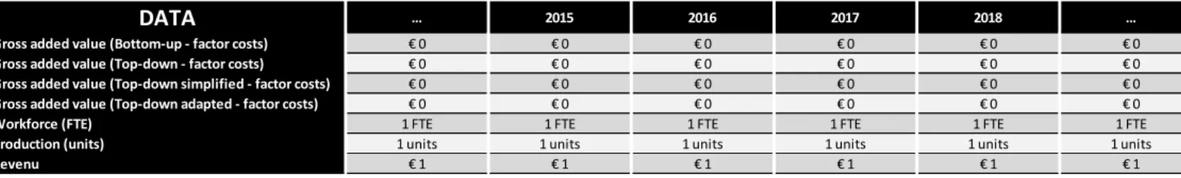
DATA … 2015 2016 2017 2018 …

Gross added value (Bottom-up - factor costs) € 0 € 0 € 0 € 0 € 0 € 0

Gross added value (Top-down - factor costs) € 0 € 0 € 0 € 0 € 0 € 0

Gross added value (Top-down simplified - factor costs) € 0 € 0 € 0 € 0 € 0 € 0

Gross added value (Top-down adapted - factor costs) € 0 € 0 € 0 € 0 € 0 € 0

Workforce (FTE) 1 FTE 1 FTE 1 FTE 1 FTE 1 FTE 1 FTE

Production (units) 1 units 1 units 1 units 1 units 1 units 1 units

2.2.4. Limitations

Although easily executable, the challenge of this method can be found in the data collection. As the required data is often not publicly available, research is highly depending on the willingness of the observed company/companies to share this data. Even data that is usually publicly available through the annual accounts is sometimes not shared, as companies with limited activities are allowed to publish a short version of the annual accounts, where revenues and costs are already submerged into a gross operational margin. In addition, another limitation that can emerge is the consolidation of activities. As such, no joint cost allocation and no joint revenue allocation is taking place, making it difficult to estimate the added value, employment and indicator values for the observed activity. A final limitation to use this method on national organisations is the uniformity of data when a trend of evolution of the past is to be studied. Indeed, when using data resulting from different accounting structures, within a company after transition or between companies using different accounting systems, it becomes difficult to compare the obtained output indicators, as they need to be interpreted within a different context linked to the corresponding used input values.

An advantage of the simplicity of the method is its usability for different organisations, sectors and even compare companies cross-border. Nevertheless, caution should be given in doing so, as once again the different used input parameters must be comparable in order for the output indicators to be comparable as well. When using data resulting from different international systems, this might prove to be very challenging. In addition, the method does not allow to make any prediction on future trends, as these are heavily dependent on the economic evolution and how the organisation and/or sector is reacting to these changes and developments. Therefore the second model takes into account a more generic impact analysis of a sector on its national economy.

2.3. Model 2: added value and employment sector-analysis (input-output)

2.3.1. General description

The second model brings a complementary view to the first one, as it takes into account the sector of rail freight transport in Belgium as a whole, and compares its impact to other sectors on the national economy. This model is developed in Deliverable 3.1 and executed in Deliverable 3.2, based on data of the main rail freight operator in Belgium, ‘Lineas’ (Troch et al., 2016; Troch et al., 2017a). The model is based on an input-output analysis, which can be used to calculate the Leontief multiplier as an economic indicator. This indicator approximates the effect of a change in final demand for an observed sector, on the total output of the economy in which the sector is operating (final demand to output indicator). In addition, this multiplier can be used to calculate an output indicator, an output-to-employment indicator and an output-to-employment-to-output-to-employment indicator. These multipliers reflect the effect of a change in respectively the output and the employment of the observed sector, on the respective output and employment of the national economy in which it is operating. This is executed in Deliverable 3.4 (Troch et al., 2018).

An input-output analysis is based on supply and demand tables, containing the outputs (supply) and inputs (demand) that are produced and required by the organizations within a national economy. Every five years, the National Bank of Belgium and the Federal Planning Office are transforming these supply and demand tables into a national input-output table containing 64 NACE sectors. The goal of this research is to extract a subcategory from one of these sectors. This can be done by using customer and supplier data of the operating companies within this subcategory, and subtracting the data from their original NACE sector. The set-up of the model, as well as the data requirements and limitations, are already explained in Deliverable 3.1 and 3.2 and will be briefly summarized in the next sections. The

main scope of the current deliverable is to explain how the calculations can be executed in Excel and Matlab.

Supply and demand tables are published yearly on the website of the National Bank of Belgium. As such, an input-output table could be generated on an annual basis. However, when the Federal Planning Office and the National Bank of Belgium are publishing the national input-output table every five years, adapted supply and demand table are included. The last edition is published in 2013, containing data of 2010. The next edition will be published end of 2018 and contain data of 2015. They include adapted supply and demand tables, as the yearly published demand table is published in buying prices including import, and should be converted to a demand table of domestic production in basic prices. This means handling margins and taxes and subsidies are filtered from the results, and import is separated from the domestic input usage. As data is not publicly available for these transitions, and the procedure is very complex and time-consuming (explaining the time delay for publishing results), this cannot be executed easily. Therefore, in order to obtain data as accurately as possible, it is recommended to collect customer and supplier data of the years in which a national input-output table is available and as such adapted supply and demand tables are publicly available as well. These are years ending in a ‘0’ or ‘5’. If no data of such years exist, an approximation of the Leontief multiplier can be calculated by adapting the public available “raw” supply and demand tables, including handling margins and import. The research shows that this results in an overestimation of the multiplier, but evolutions within the multiplier itself remain stable and can be observed with this method. The calculation of the indicators is executed in a similar way as when the adapted supply and demand tables are used.

2.3.2. First step: collecting supplier and customer data

A first step to calculate the Leontief multiplier indicator is to collect supplier and customer transactions data from the desired sub-sector. In the executed research, supplier and customer transaction data of the incumbent rail freight operator ‘Lineas’ was used as a representation of the rail freight sector in Belgium. Data from multiple companies representing a sub-sector can be equally used by simply adding them together. Customer/Supplier data (sales/purchases) should contain the following information:

 Customer/Supplier company name  VAT number

 Sales/Purchase amount in EUR

In order for this data to be usable, each customer and supplier must be linked to its NACE code according to the NACE-BEL classification. This is necessary to know from which NACE sector the input / output transaction should be subtracted in the supply and demand tables. Linking an organisation to its NACE code can be done by using the VAT code. A list of all national organizations is publicly available, linking the VAT code of an organization to its primary NACE code. These export files are made available through the website (https//www.brain-trains.be).

As VAT codes are often published in the format “BExxxxxxxxx”, and the VAT codes within this database are in the format “0xxx xxx xxx”, a first transition should be made, as spaces are taking into account when using excel functions. This can be easily done with the VAT converter in excel, for which a template has been provided together with this deliverable and is available through the website (https://www.brain-trains.be).

In a second tab sheet, a list of existing connections for the observed rail freight operator ‘Lineas’ is also made available for future research. The template can be used by pasting the VAT numbers in column A. Selecting all VAT numbers, the function ‘text to columns’ should be selected in the ‘DATA’ menu. The option ‘Fixed width’ should be selected. Splitters can be added after the ‘BE’ indication and for each

group of three numbers. When finishing, the VAT number is split over the columns A, B, C and D. Now the ‘BE’ indication can be replaced by a ‘0’ in order to obtain the VAT number in a useable format. A third tab sheet allows linking the VAT number in the new format to the primary NACE code. When entering the VAT for lookup in column D, the file will automatically look for existing connections and show the results in column E ‘NACE exists’. For the remaining unavailable NACE codes (#N/A), the export files can be used. This export of national organizations linked to their primary NACE classification is split into 15 categories, each grouping a number of NACE codes. The template in Excel is taking into account the same groups of NACE codes in columns H to V. As such, each column must be linked to this export file, by entering a ‘VLOOKUP’ formula:

= VLOOKUP(A,B,C,D)

 With A = The VAT for lookup (= Dx, with x the row number)

 With B = The table in which A should be looked for, being the export file (=’[export file name]Lijst’! $D$2:$E$1000000

Example: For column H (1-29) this is export file ‘NACE 1-29.xlsx’. As such, B in the

formula would be: '[NACE 1 - 29 (done).xlsx]Lijst'!$D$2:$E$1000000

Caution! When executing, a prompt box will appear to select the correct file. Therefore,

make sure that the export files are available somewhere on your computer, in order to select the correct file.

 With C = 2  With D = FALSE

The template in excel will automatically convert the found NACE codes into a simplified version in column F. In case a company is still left without a NACE code after this process, the VAT number can be looked up in the CBE Public Search (https://economie.fgov.be) in order to obtain the primary NACE classification.

After all companies are linked to their primary NACE classification, the Excel template is automatically creating a PIVOT in the fourth tab sheet.

2.3.3. Second step: adapting the supply and demand table

As soon as the Customer Pivot and the Supplier Pivot of an organization are generated, the corresponding national supply and demand tables can be adapted.

In the corresponding demand table for the year of which customer and supplier data has been used, an additional sector can be created by adding one row and one column. In our example, we will call this sector ‘X’. The newly created row reflects the product of sector ‘X’, whereas the column represents the sector as an entity. The data of the customer PIVOT table of each organisation of sector ‘X’ is placed in the newly-created row of sector ‘X’, and deducted from the original NACE sector of this company. The data of the supplier PIVOT table of each organisation is placed in the newly-created column of sector ‘X’, and deducted from the original NACE sector of this company.

In the corresponding supply table for the year of which customer and supplier data has been used, an additional sector can be created by adding one row and one column. In our example, we will call this sector ‘X’. The data of the customer PIVOT table of each organisation of sector ‘X’ is placed at the cross point of the new column and row for sector ‘X’. This is the amount that the sector produced of its offered product to the domestic market. The amount is deducted from the cross point of the original sector of the respective companies that are taken into account for the new sector ‘X’.

2.3.4. Third step: creating the new input-output table

When the supply and demand tables have been adapted by adding the newly investigated sector, the new 65x65 input-output matrix can be recalculated. As the supply and demand tables are product-to-sector matrices, and the input-output matrix is a product-to-sector-to-product-to-sector matrix, for each product-to-sector combination ,the supply of sector 1 must be multiplied with the relative demand of that supplied product by sector 2. For a 65x65 matrix, this results in 4.225 calculations. To do this easily, the Excel template is providing a format in the fifth tab sheet that can be used to simplify this process to ‘only’ 65 calculations. The following inputs need to be entered:

 Column C: the supplies of sector X – this needs to be adapted 65 times  Column G to BS: the demand table

 Column BW: the total supply

The Excel is performing automatic calculations and presents the results in row ‘BY68’ to ‘EK68’. This needs to be transferred to the input-output table, as the row of the sector for which the supplies have been entered in column C. For example, if the supplies of sector 5 have been entered, the results are in the fifth row of the new input output table. As such, the full 65x65 input-output matrix can be easily calculated by entering the 65 supply vectors in column C sequentially.

The input-output matrix that has been created is showing the output of each row sector towards another domestic column sector, or the domestic input that a column sector is requiring from a row sector.

2.3.5. Fourth step: calculating the Leontief multiplier

Once the new input output table with 65 sectors is created, the Leontief multiplier can be calculated. This is done in two steps, by preparing the necessary matrices in Excel and running a script in Matlab. First, preparations for the Leontief multiplier calculations can be made in the provided Excel template, more specifically in the sixth tab sheet ‘Leontief input’. The calculated input-output table can be placed in matrix ‘A2:BM67’. This will automatically calculate a total in column ‘BO’. Column ‘BP’, ‘BQ’ and ‘BR’ contain data on final consumption of respectively households, non-profit organizations and the government. For most sectors, this data can be copied from the demand table. For the newly created sector ‘X’ that is examined, data will need to be collected or assumptions will need to be made to split the final consumption from the original sectors. The same procedure is valid for columns ‘BT’ to ‘BW’, containing respectively the investments, changes in stock and export within Eurozone, within the European Union and outside of the European Union. Export of sector ‘X’ can be collected through the supplier data obtained from the observed organizations reflecting sector ‘X’. When all information is completed, a final total will be automatically calculated in column ‘BX’.

Second, the matrix for the Leontief multiplier approximation can be calculated. To do this, the following formula needs to be calculated, as described in D3.1 and 3.2:

L = (C – A * B-1₎-1

 A = the input-output matrix with all intermediary deliveries  B = the diagonal matrix with total inputs /outputs

 C = the identity matrix for the number of sectors involved  L = the Leontief matrix

Within the sixth tab sheet of the Excel template, these matrices are automatically prepared. The calculated input output matrix ‘A2:BM67’ corresponds to matrix ‘A’ in the formula. The yellow matrix ‘CA3:EM67’ is the diagonal matrix of the total input/output, corresponding to matrix ‘B’. This matrix is also calculated automatically. As this is done by an array function in excel, when executing manually, the full matrix needs to be selected and recalculated with the command ‘Ctrl + Shft + Enter’. These matrices can be entered in the Matlab script, which is also included with this document and available on the website www.brain-trains.be. Within this script, the matrices ‘A’ and ‘B’ can be copy pasted from Excel. Matrix ‘C’ can be included with the matrix function on the left taskbar, indicating the number of rows and columns, and by choosing the ‘identity matrix’ as ‘type’. With the button ‘insert matrix’, the identity matrix ‘C’ can be generated. Take note that this process needs to be repeated every time the script is opened, as the identity matrix is not stored automatically when saving the script. When the three matrices ‘A’, ‘B’ and ‘C’ are inserted in the script, it can be run by selecting each next formula sequentially and executing it by clicking ‘Enter’. First, matrix ‘B’ will be inverted and stored as matrix B1 (L = (C – A * B1)-1_{). Secondly, matrix ‘A’ and ‘B1’ are multiplied creating matrix ‘AB1’ (L = (C – AB1)}-1_).

Thirdly, this newly created matrix is deducted from the identity matrix, creating the matrix ‘TOT’ (L = TOT-1_{). Finally, this matrix is inverted to obtain the Leontief matrix ‘L’ or ‘TOT}-1_{’. This matrix can be}

exported to excel by double clicking the result and selecting the export function.

As soon as the Leontief matrix is obtained, the Leontief multiplier approximation indicator can be calculated for each sector by taking the sum of the corresponding column. The obtained result estimates the total effect on the national economy when the final demand of the studied sector is increased by one unit.

2.3.6. Fifth step: converting to an employment multiplier

In a final fifth step, three additional indicators can be generated, estimating the impact of a change on the national economy in terms of output and employment.

A first indicator is the output-to-output multiplier, or the net multiplier. This approximation is obtained by dividing each element in the Leontief matrix ‘L’ by the diagonal element of the respective sectors. This can be executed easily in the seventh and final tab sheet of the template in Excel. When entering the Leontief matrix (B3:BN67), the template is automatically calculating the diagonal element in column ‘BP’ and presents the results of the net multiplier in matrix ‘BR3:ED67’. The actual net multipliers are presented in row ‘BR69:ED69’. These net multiplier indicator approximations are presenting the total change in output of the national economy when the output of a sector is increased by 1 unit.

A second indicator is the output-to-employment multiplier, indicating the effect on the employment of the national economy when the output of a sector is increased by one. This indicator requires additional data to be provided in the excel template. Column ‘EF’ is automatically transmitting the total output values from the Leontief tab sheet. Column ‘EG’ needs data on the employment of each sector and should be completed. This data can be found on the site of the National Bank of Belgium, per sector and corresponding NACE classification. When this data is completed, column ‘EH’ is automatically calculating the necessary employment per output generated. This parameter is needed to calculate the output to employment matrix ‘EJ2:GV67’. The output to employment multiplier indicator is presented in row ‘EJ69:GV69’.

A third and last additional indicator is going one step further and evaluates the effect of an increase in one additional employment unit in a sector on the national employment values. This approximation is automatically generated in matrix ‘GZ2:JL67’. The total employment-to-employment indicator is presented in row ‘GZ69:JL69’.

3. User guide of the methodology of WP4: sustainability impact

3.1. Introduction

The research carried out within the framework of the Work Package 4 (WP4 - sustainability impact of intermodality) of the BRAIN-TRAINS project has had several stages. In a first stage, we have analysed the environmental impacts of rail freight transport (distinguishing between electric and diesel traction), inland waterways transport and road freight transport independently. Moreover, a comparison between the environmental impacts of these inland freight transport modes has been performed. It should be noted that as the study of the different scenarios has progressed and new data have been collected, the method used has improved and therefore the results have been updated. Thereby, the first results in energy consumption, direct emissions and impact assessment have been explained in the deliverable D.4.2 of the BRAIN-TRAINS project (Merchan et al., 2017a). Afterwards, the results in rail freight transport and road freight transport have been updated in the deliverable D.4.3 (Merchan et al., 2017b). This is because the information collected on railway infrastructure had been fully modelled and the values of energy consumption in road transport had been revised as a result of enhanced load factors. Finally, the results in impact assessment of road freight transport have been updated again in the deliverable D.4.4 (Merchan et al., 2018) as a result of the improvement in the method of calculating road infrastructure demand.

In a second stage, we have carried out a study of the environmental impacts related to intermodal rail freight transport. For this, we have studied three consolidated intermodal rail-road routes in Belgium in the deliverable D.4.3 of the BRAIN-TRAINS project (Merchan et al., 2017b). The objective of this analysis was to compare the environmental impacts of these intermodal routes depending on the freight transport mode chosen (rail or road transport) for the major part of the intermodal route.

In a third stage, we have analysed how the increase of rail freight transport as a result of the possible development of the intermodal rail freight transport affects the environmental impacts of the modal split of inland freight transport in Belgium. For this, we have studied an increase of rail demand of 133%, 64% or 10% for the best, medium and worst-case scenarios in the deliverable D.4.4 of the BRAIN-TRAINS project (Merchan et al., 2018).

The purpose of this deliverable is to develop a user guide of the methodology developed by WP4 to determine the environmental impacts of both intermodal freight transport in Belgium and the three scenarios developed for the year 2030.

3.2. Methodology

The Life Cycle Assessment (LCA) methodology has been chosen to analyse the environmental impacts of the intermodal freight transport in Belgium, which includes the LCA of rail freight transport (distinguishing between electric and diesel traction), IWW transport and road freight transport. The LCA methodology allows studying complex systems like freight transport, providing a system perspective analysis that allows assessing environmental impacts through all the stages of the intermodal freight transport system (transport operation, vehicle and infrastructure), from raw material extraction, through materials use, and finally disposal.

Furthermore, the LCA approach allows analysing the overall life cycle of the energy carrier. Thereby, we consider the environmental impacts related to the use of energy (e.g. diesel or electricity) starting from the raw materials extraction (e.g. oil or uranium), continuing with energy generation (e.g. diesel refining or electricity production) and ending with the energy distribution to the traction unit (locomotive, barge or lorry). Besides the assessment of the environmental impacts related to the energy consumption

during the transport operation, our LCA study includes the emissions and energy and raw material consumptions from the construction and maintenance of transport infrastructure and the manufacturing and maintenance of transport vehicles.

A LCA study comprises four stages: First, the goal and scope definition.

The second stage of a LCA is the inventory analysis, collecting data directly from Infrabel and B-Logistics (rebranded to Lineas, April 2017) in the case of rail freight transport and complementing the information using the Ecoinvent v3.1 database (Weidema et al., 2013). The model used in Ecoinvent V3.1 has been adapted to the Belgian situation in the case of both IWW transport and road transport (using the calculated transport parameters of tonne-kilometres, load factor, payload, number of vehicles, and characteristics of infrastructures for example).

The third stage is the impact assessment. All calculations in our study have been made with the SimaPro 8.0.5 software using the Life Cycle Impact Assessment (LCIA) method “ILCD 2011 Midpoint+” (version V1.06 / EU27 2010), which is the method recommended by the European Commission (European Commission, 2010). “ILCD 2011 Midpoint+” is a midpoint method including 16 environmental impact indicators.

The fourth stage is the assessment of the results obtained in the previous stages.

3.2.1. Goal and scope definition

The LCA study carried out within the framework of the WP4 aims to analyse the environmental impacts of intermodal freight transport in Belgium and the different scenarios developed for the year 2030. The functional unit chosen has been “one tonne-kilometre of freight transported” in the different modes of transport.

3.2.2. Life Cycle inventory

Figure 6 presents the stages considered in our study for the rail freight transport, IWW transport and road freight transport.

A detailed study of the rail freight transport has been conducted, collecting data directly from Infrabel (the Belgian railway infrastructure manager) and B-Logistics (rebranded to Lineas, April 2017), which is the main rail freight operator in Belgium. The rail freight system has been divided in three sub-systems: rail transport operation, rail infrastructure and rail equipment (locomotives and wagons).

For the rail transport operation sub-system, the specific energy consumption of electric and diesel trains has been determined separately. Upstream emissions related to the production and distribution of the energy to the traction unit and the direct emissions during the rail transport activity have been determined.

FIGURE 6: INLAND FREIGHT TRANSPORT SYSTEM BOUNDARIES CONSIDERED IN OUR STUDY

SOURCE: OWN ELABORATION BASED ON SPIELMANN ET AL., 2007

In the case of indirect emissions from electric trains, in order to adjust as closely as possible the environmental impact related to the yearly electricity consumption, and since the electricity supply mix varies widely over the years, our LCA study uses the electricity supply mix in Belgium corresponding to the appropriate year. Three types of direct emissions produced during the rail transport operation have be distinguished: the exhaust emissions to air related to the diesel combustion in locomotives, the direct emissions to soil from abrasion of brake linings, wheels and rails and the sulphur hexafluoride (SF6)

emissions to air during conversion of electricity at traction substations.

As shown in Figure 7, the subsystem rail infrastructure includes the processes that are connected with the construction, maintenance and disposal of the railway infrastructure. We have collected data from Infrabel and literature sources relative to the Belgian railway infrastructure. This comprises information on the materials and energy used in the construction of the railway network (including track, tunnels and bridges) such as rails, sleepers, fastening systems, switches and crossings, track bedding or overhead contact system for example. The maintenance of the Belgian railway infrastructure has been analysed as well. Therefore, the maintenance works such as rail grinding, rail renewal, sleeper and fastening system renewal, switches and crossing renewal, ballast tamping, ballast renewal, ballast cleaning and weed control are taken into account. We have considered in the maintenance of railway infrastructure both the fuel consumption and exhaust emissions from the machinery used in the maintenance and the new materials used in the track renewal. We have also included in our study the end-of-life of the railway infrastructure and the land use in the Belgian railway network. Most of the elements are recycled such as the ballast that is reused as material for backfill and the wooden sleepers that are incinerated with energy recovery.

The life cycle phases of manufacturing, maintenance and disposal of rail equipment (locomotives and wagons) are taken into account in our study as well.

FIGURE 7: LIFE CYCLE ASSESSMENT OF THE RAILWAY INFRASTRUCTURE

In the case of both inland waterways transport and road transport in Belgium, the Ecoinvent V3.1 database has been used as a model (Weidema et al., 2013). Analogously to the rail transport system, for the LCA of inland waterways transport, all life cycle phases of inland waterways transport operation, inland waterways infrastructures (including canals and the Port of Antwerp), and manufacturing and maintenance of the barge are included. Information relative to the total annual freight moved by inland waterways transport in Belgium by barge type, fuel consumption in the vessel transport operation and waterways infrastructure characteristics for several years have been collected. For the LCA of road transport, all life cycle phases of road transport operation, road infrastructure, and manufacturing and maintenance of the lorry are included. Information relative to the total annual freight moved by road transport in Belgium by weight classification and heavy duty vehicle technology type, fuel consumption in the road transport operation and road infrastructure characteristics for several years have been collected.

Tables 1, 2 and 3 present the main data used to develop the Life Cycle Inventory of rail, IWW and road freight transport.

TABLE 1. MAIN DATA USED TO DEVELOP THE LIFE CYCLE INVENTORY OF RAIL FREIGHT TRANSPORT

Data Main sources

Transport operation

Total annual energy consumption SNCB (2009, 2013 and 2015)

Rail freight traction share Vlaamse Milieumaatschappij (VMM) (2008, 2009, 2010, 2012 and 2013)

Electricity supply mix Eurostat statistics (2017) Emission factors for direct emissions Spielmann et al. (2007)

Sulphur content of diesel EU Fuel Quality Monitoring (2012)

Railway Infrastructure

Length of railway lines in Belgium Eurostat statistics (2017) Transport performance (tkm) SNCB (2009, 2013 and 2015) Operating performance (Gtkm) Eurostat statistics (2017) Kilometric performance (train-km) Eurostat statistics (2017)

Construction, maintenance and disposal

IBGE (2011); Kiani et al. (2008); Infrabel (2007, 2011, 2014 and questionnaires); Schmied and Mottschall (2013); Spielmann et al. (2007); Tuchschmid et al. (2011) and UIC (2013)

Rolling stock Population of locomotives and wagons

Eurostat statistics (2017) and SNCB (questionnaires)

Manufacturing, maintenance and disposal Ecoinvent database (2013)

TABLE 2. MAIN DATA USED TO DEVELOP THE LIFE CYCLE INVENTORY OF INLAND WATERWAYS TRANSPORT

Data Main sources

Transport operation

Class-specific fuel consumption of barges Service Public de Wallonie (2014)

Carrying capacity of each vessel class Institut pour le Transport par Batellerie (ITB) (2006, 2007, 2008, 2009, 2010, 2011 and 2012) Emission factors for direct emissions Spielmann et al., (2007)

Inland waterways

and Port

Length of inland waterways Eurostat statistics (2017) Transport performance (tkm) Eurostat statistics (2017) Incoming and outgoing Port of Antwerp Antwerp Port Authority (2016) Construction, maintenance and disposal Ecoinvent database (2013)

Barges Population of barges

Institut pour le Transport par Batellerie (ITB) (2006, 2007, 2008, 2009, 2010, 2011 and 2012) Manufacturing, maintenance and disposal Ecoinvent database (2013)

TABLE 3. MAIN DATA USED TO DEVELOP THE LIFE CYCLE INVENTORY OF ROAD FREIGHT TRANSPORT

Data Main sources

Transport operation

Average diesel consumption TRACCS database (2013)

Maximum payload TRACCS database (2013)

Transport performance (tkm) COPERT (2016)

Emission factors for direct emissions Spielmann et al. (2007) and EMEP/EEA (2013)

Road infrastructure

Length of road infrastructure Eurostat statistics (2017) Construction, maintenance and disposal Ecoinvent database (2013)

Lorries

Population of lorries COPERT (2016)