Structural optimisation of steel frames for industrial applications

Structural optimization of steel frames for industrial applications

Mathonet Vincent M & S Department, University of Liège, ULg

Liège, Belgium [email protected]

Degée Hervé M & S Department, University of Liège, ULg

Liège, Belgium

Habraken A.-M. M & S Department, University of Liège, ULg

Liège, Belgium

Tossings Patricia ASMA Department University of Liège, ULg

Liège, Belgium Delhez Eric

ASMA Department University of Liège, ULg

Liège, Belgium

ABSTRACT

The paper reports the first results of a work carried out in close collaboration between Astron Buildings SA, a manufacturer of industrial steel buildings, and different groups of civil engineers and mathematicians of the University of Liège to develop an automatic design method for structures with tapered members. This research aims at improving the current method of trial- error followed by experienced engineers to optimize the frames constrained by a chosen national construction code and the technological constraints of the producer.

The main benefit of this collaboration arises through the application of a mathematical algorithm based on the sequential quadratic programming method (SQP) in order to reduce, in the first step, the weight of the building, under the great number of constraints. The second step, not yet started, will be devoted to the minimization of the real cost of the frame. This report introduces the first results of this industrial application.

INTRODUCTION

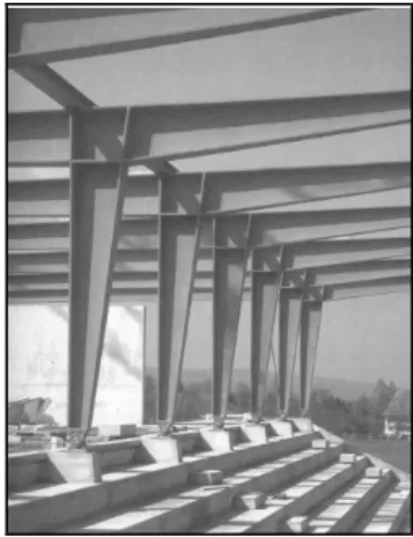
Astron Buildings is the actual European leader on the steel building ma rket. Experienced for 35 years in industrial and commercial applications, its products are perfectly suited to a wide range of projects from simple frames and elementary configurations up to complex modules. In this very competitive market, Astron Buildings distinguishes itself by its original process based on tapered members and not laminated members (see Figure 1). Much raw

material can be saved in this way but additional manufacture costs are induced. The approach is nevertheless cheaper than laminated solutions if the design is well studied. The design procedure is therefore very critical but is complicated by the large number of constraints that must be taken into account.

Figure 1: tapered section elements.

The first constraints appear at the production stage. The profiles are manufactured by Astron in two factories in Luxembourg and in the Czech Republic where the rafters and columns composing the frames are also dimensioned and fabricated. The height, width and thickness of the webs and flanges of these elements are allowed to change along a given element. At this stage, the

dimensions of the profiles are limited by the production constraints and by the technological limits of the cutting press and automatic electric welders dedicated to the handling of these profiles. The second category of constraints is related to the resistance and the stability of the structure. The design must indeed be checked against these resistance and stability conditions, that are imposed by national and/or European codes.

To cope with the numerous calculations required, the design department of ASTRON has developed a software — the APS code — to check the resistance and the stability conditions at each section of the frame and to ease the identification of the required improvements of the design.

Currently, the strong competition in the steel construction market pushes engineers to optimize the cost of the structures. To do so, they rely on their experience and optimization tables (elementary optimization rules) or follow a ‘trial and error procedure’, to reduce the cost. This time consuming and empirical method offers no guarantee to identify the optimum design.

The optimization procedure could however be improved by a computerized automatic strategy. This fact motivated the start of a collaboration with mathematicians and engineers of several departments of the University of Liège to develop an automatic optimization method based on a mathematical algorithm. The results achieved after a first feasibility study of this approach give confidence about the ultimate success of the project.

The first sections of the paper provide an introduction to the formulation of the problem and to the algorithm that is used for optimization. In the third section, we discuss particular aspects of the application of the optimization algorithm to the problem. Preliminary results are then presented and discussed. Conclusions and perspectives close this paper.

PROBLEM FORMULATION

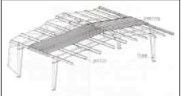
Before addressing the general problem of the optimization of an arbitrary structure, a simple (but representative) configuration has been selected as test case for a feasibility study. The basic case that is studied here is the classical frame shown in Figure 2 — an AZM1 structure in the ASTRON terminology —.

The aim of the optimization is to identified the cheapest structure. The quantitative assessment of

the global cost of a structure is a very difficult exercise however. Not only the cost of the raw material, but also the cost of manufacture, handling and transport should be taken into account. This cost evaluation requires an in depth analysis of the different steps of production and appropriate imputation rules for the various direct and indirect costs. This study is currently under way. As a first step, however, the weight of the structure is taken as the objective function of the optimization. The weight is easily expressed in terms of the dimensions of the different beams composing the frame. The formula can be improved by taking into account the weights of haunches and connectors. These are however neglected in the feasibility phase. The work concentrates thus on the dimensioning of the webs and flanges of the 4 elements (2 columns, 2 rafters) composing the AZM1 frame.

Figure 2: AZM1 structure.

The formulation of the constraints begins with the constraints generated by the national steel construction code. The Eurocode 3, selected in this optimization problem, imposes the verification of 13 ratios at a defined number of sections of the frame as well as limitations on the maximum displacements at the top of the columns and at the top of the roof. These Eurocode 3 constraints must be satisfied for various combinations of loads.

The other constraints taken into account in the formulation are the technological constraints associated with the production of the elements and the erection of the building. Among these constraints we can list :

§ equality of the widths of the flanges along each beam,

§ maximum slope between the flanges, § minimum thickness for welding

§ limit dimensions imposed by steel supplier,

§ minimum dimensions so as to avoid the flange buckling caused by the weldings, § dimensions prescribed by the customer’s

application,

§ continuity of heights.

SQP ALGORITHM FORMULATION

The program solves optimization problems such that:

min f(x) under the contraints gi

( )

technological and stability constraints.

Quadratic subproblem

The mathematical algorithm used to solve the optimization problem is based on the sequential quadratic programming method (e.g. Fletcher, 1987). This method amounts to the solution of a serie of quadratic sub-problems based on local quadratic models of the objective function and the constraints. At each step of the iterative resolution, the quadratic sub-problem

min f(xk) + ∇fT(xk)(x-xk) + 2

1 (x-xk)TW(xk)(x-xk)

(2)

under the linear constraints

gi(xk)+∇giT(xk)(x-xk)

≥

is build around the current iterate xk.

The values of the objective function f(xk) and of

its gradient ∇f(xk) appearing in (2) are available in

analytical form. The values of the constraints gi(xk) at the current iterate are obtained by running

the APS code. The gradients ∇gi(xk) are

computed by finite differences from repeated runs of the APS. The matrix W(xk) denotes an

approximation of the Hessian matrix of the Lagrangian function L(x, λ) = f(x) -

∑

where λi (i=1,2,...,ncon) are the so-called

Lagrange multipliers associated to the different constraints. This matrix W can expressed as Wf

+ Wc where Wf and Wc are associated

respectively with the second derivatives of f and

of the gi’s one. The former are available in

analytical form while the latter must be approximated using a BFGS approach (e.g. Fletcher, 1987).

Resolution of the quadratic sub-problem Once the quadratic sub-problem (2)-(3) is available, a feasible point is sought for the linearized constraints (3). A classical simplex method (e.g. Dantzig, 1963) is used for this purpose. This feasible point serves then as an initial point for an iterative resolution of the quadratic sub-problem.

The resolution of the quadratic sub -problem proceeds using an active constraints strategy. The constraints in (3) that are satisfied with the equality at the feasible point are called active. The problem

min f(xk)+∇fT(x-xk)+ 1₂(x-xk)TW(x-xk) (5)

under the nc active linear constraints (nc≤ncon)

gi(xk)+∇giT(x-xk)=0 (i=1,2,...,nc) (6)

is then solved using a reduced gradient approach. In other words, the minimum of the quadratic objective function (5) is sought in the linear subspace defined by the active constraints. An orthonormal basis for this subspace is generated using a QR matrix decomposition of the matrix A formed by the components of the nc gradients ∇gi of the active constraints.

When solving (5)-(6), some of the non active constraints can become active. Also, it may be necessary to remove some of the constraints from the active set to achieve a further reduction of the objective function. This can be checked by checking the sign of the Lagrange multipliers given by

λ = AT_∇f

(7) As a result, the set of active constraints is updated repeatedly until a minimum is found which satisfies all the (active and non active) constraints (3).

Global convergence and merit function The solution of the quadratic sub-problem is used to define a research direction dx along which the minimum of the merit function

F(x) = f(x)+ν

∑

[

]

is sought using a line search procedure. To save computer resources, an approximate line-search is carried out. The merit function F(xk+αdx) is

computed for different values of α and the line search is stopped when the Armijo conditions are satisfied, i. e. when a sufficient decrease of F is obtained. The point xk+αdx is then taken as the

new iterate xk+1.

The line search procedure based on the exact merit function F can be shown to ensure global convergence towards the minimum of the original problem (1) on the condition that the penalty parameter ν is such that

ν ≥

∑

λ

)

(

where λi are the Lagrange multipliers at the optimum.

Ending and convergence

The algorithm stops when a local optimum is reached, i.e. when the gradient of the Lagrangian function is below a predefined tolerance value or when the line-search fails to produce any improvement of the objective and merit functions.

ALGORITHM APPLICATION

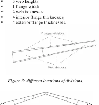
The Astron’s application takes place in a routine called ‘simul’. This routine computes the objective function, the constraints and their derivatives that are required for the optimization. The parameters identified for the design of the frame are gathered in a vector whose size must be constant during the optimization process. In the usual empirical practice, designers can divide the web and flanges into sections of various dimensions. The location of the web and flanges divisions does not need to correspond and their number can be different for the web and flanges. Figure 3 shows an example of such divisions of a rafter. A variable number of divisions could not be managed during the optimization, each element is therefore divided into 4 sections of equal length.

Figure 4 presents the selected definition of frame dimensions. The design of each element can be defined by 18 parameters:

§ 5 web heights § 1 flange width § 4 web ticknesses

§ 4 interior flange thicknesses § 4 exterior flange thicknesses.

Figure 3: different locations of divisions.

Figure 4: Frame divisions.

Figure 5: 1/4 element variables names.

This distribution already allows the simplication of two technological constraints:

§ the heights continuity so as to avoid web step-up.

§ the common width of flanges along a beam.

The parameters vector is thus dimensionned to contain the 4 x 18 parameters, this choice enables to add additional elements to be optimized in the future.

The objective function, its derivatives, the constraints and their derivatives are evaluated for

each call of ‘simul’. The weight is an analytic relation, its first and second order derivatives are easily established analytically. The definition of the technological and Eurocode constraints takes place in the second part of the routine. These can be divided in two categories:

§ the contraints expressed by analytic relations

§ the contraints computed by calling the APS code.

Constraints like maximum slope between the flanges fall in the first group ; they can be exp ressed by formulations similar to:

g(x) = ∠flange - 15 ≥ 0 (9)

The second category is made of the Eurocode ratios and the maximum displacements. The original implementation of the APS did not provide any direct access to these data. Modification of these routines have therefore been implemented in order to output the adequate ratios and displacements into a structured data file. The new implementation short-cuts useless interventions of the operator to automate the execution of the code. The constraints computed by APS are expressed as differences that must remain non negative. For example,

g(x) = 1 - Ratio ≥ 0 (10) (Eurocode 3 imposes Ratio ≤ 1)

The last part of the routine ‘simul’ is devoted to the evaluation of the first order derivatives of the objective function and constraints. The derivatives of the weight of the structure are evaluated analytically. For the constraints evaluated by APS, the computation of the derivatives is done by finite differences. The constraints are first computed by repeated calls of the APS for positive and negative perturbations of the parameters and the derivatives are computed subsequently as on perturbati 2Ratio Ratio x ) x ( gi × − = ∂ ∂ + − ₍₁₁₎

The number of APS runs required for the evaluation of the derivatives of the Eurocode constraints is thus given by twice the number of optimized parameters (running time of 1 execution: 1-2 sec. on the M&S department’s machine). This second method used to calculate the sensitivity matrix is the weak point of the optimization: the time consuming ‘APS’

execution when the computation of Eurocode contraints derivatives is required. A flag allows to skip the computation of the derivatives at some points of the algorithm, hence reducing optimization time.

The structure of the routine ‘simul’ is suitable to problems of any size. The basic frame asks for the verification of the 13 Eurocode ratios at 90 sections, hence a total of 90 x 13 constraints in addition to the technological constraints. A frame optimization for one load combination is therefore constrained by more than 1000 constraints and the complete optimization problem under the whole set of load combinations by more than 5000 constraints.

RESULTS OF FIRST OPTIMIZATIONS In the feasibility study much time was spent in the establishing of the analytic relations, in the programming of the derivatives loops and in modifications of the Astron’s program.

Debugging and validation of the integration of the APS and SQP codes was done on the simplified problem of the parameters optimization of one single beam under its Eurocode constraints. This simplification has permitted to reduce the optimized parameters number to 18 under the restriction of its 14 sections verification and thus 182 constraints. This choice permits to:

§ save time during the develo pment, § locate easily the troubles in the routines. The first optimization, concerning the left column under its Eurocode constraints, is started with an input file containing random parameters. These initial parameters violate some constraints, the initia l weight is quite low. About 10 iterations are sufficient to reach a local optimum. Figure 6 shows the evolution of the objective function and the number of violated constraints during the optimization process . The dimensions of the left column are thus optimized, respecting its 182 Eurocode constraints for one load type.

In a second step, additional constraints are introduced: maximum displacement and maximum slope between the flanges in addition to the Eurocode constraints. The optimization quickly obtains a reduced weight.

Figure 6: objective function of the beam. Only one constraint limits this reduction: the maximum lateral displacement at the top of the left column. The optimum is found from a line search along the constraint direction. The weight during the optimization is presented at Figure 7.

Figure 7: weight=f(iterations)

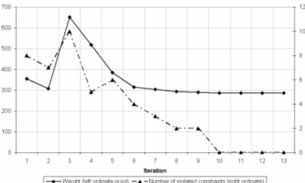
Once carefully checked in the simplified framework of a single column, the optimization code is applied to the whole AZM1 frame under one load type. The technological constraints aren’t yet accounted for and only the 1170 Eurocode constraints limit the problem. This first optimization under a large number of parameters (72) and a lot of contraints aims at testing the behaviour and the management of the algorithm with a very constrained application. The initial parameters are the parameters optimized by Astron’s engineer with their empirical method. They are optimized with respect to the constraints for 5 different loads combinations and the technological constraints. The two optimized results can’t be compared:

§ one is obtained for 1 load combination, the other 5. The last one is more constrained.

§ one is computed for a cost optimization and the other compared to the weight optimization.

This initial point is realistic and is an interesting starting point. Figure 8 shows the convergence of the optimized weight around 1780 kg.

Figure 8: obj. function with violated constraints

Memory problems appeared when enlarging the problem from 1 element to 4 elements. The simplex routine used for the identification of an initial feasible point uses indeed a double precision matrix of 1200x1200 ; i.e. too large to be managed by the computer. As a first step, the precision of this matrix is reduced to simple precision. A reduce storage dual simplex method will be used in the future to save memory.

CONCLUSION AND PERSPECTIVES The feasability phase is concluded with encouraging results. The algorithm reaches a consequent and efficient minimization of the weight, taking into account a large number of constraints. Improvements of the different optimization and data handling routines will however be implemented in the near future to cope with an unlimited number of constraints.

These presented results introduce the first phase of a frame optimization: the actual parameters resulting of the optimization are continuous parameters. Practically, only discrete dimensions can be provided by the steel producer, the optimized values have thus to be converted to discrete values from a catalog. In general, the optimum obtained with continuous parameters does not correspond to the optimum of the discrete case. The second phase of development will rely on a branch and bound method to cope with this discrete optimization problem. In a third

and ultimate step, the code will be adapted to optimize the global cost of a frame.

ACKNOWLEDGMENTS

The authors are deeply grateful to ASTRON Buildings SA for its financial support of this work and they express their appreciation to C. Weinquin, M. Braham, M. Sarlet and A. Wantz for their kind help in the course of this research.

As members of the National Fund for Scientific Research (Belgium), A.-M. Habraken, H. Degée thank this Belgian research fund for its support.

REFERENCES

§ Dantzig, G.B., 1963. Linear Programming and Extensions. Princeton, N.J. : Princeton University Press.Fletcher, R., 1987.

§ Practical methods of optimization, 2nd Edition.John Wiley & Sons.

§ A. Hirt, M., Chrisinel, M., Charpentes Métalliques, Traité de génie civil 11, Presse polytechnique et universitaire romande.