Laboratoire d'Analyse et Modélisation de Systèmes pour l'Aide à la Décision
CNRS UMR 7024
CAHIER DU LAMSADE
206
“Additive difference” models without additivity and subtractivity
‘Additive difference’ models without
additivity and subtractivity
1
D. Bouyssou
2CNRS – LAMSADE
M. Pirlot
3Facult´e Polytechnique de Mons
1We thank Th. Marchant for helpful comments on an earlier draft of this text. Part of this work was accomplished while Denis Bouyssou was visiting the Ser-vice de Math´ematiques de la Gestion at the Universit´e Libre de Bruxelles (Brus-sels, Belgium). He gratefully acknowledges the warm hospitality of the Service de Math´ematique de la Gestion as well as the support of the Belgian Fonds National de la Recherche Scientifique and the Brussels-Capital Region through a “Research in Brussels” action grant. The other part of this work was accomplished while Marc Pirlot was visiting LIP6–Universit´e Pierre et Marie Curie and LAMSADE– Universit´e Paris Dauphine (Paris, France) thanks to visiting positions in these two institutions and a grant from the Fonds National de la Recherche Scientifique. He gratefully acknowledges this support.
2LAMSADE, Universit´e Paris Dauphine, Place du Mar´echal de Lattre de Tas-signy, F-75775 Paris Cedex 16, France, tel: +33 1 44 05 48 98, fax: +33 1 44 05 40 91, e-mail: [email protected].
3Facult´e Polytechnique de Mons, 9, rue de Houdain, B-7000 Mons, Belgium, tel: +32 65 374682, fax: + 32 65 374689, e-mail: [email protected]. Corresponding author.
Abstract
This paper studies conjoint measurement models tolerating intransitivi-ties that closely resemble Tversky’s additive difference model while replacing additivity and subtractivity by mere decomposability requirements. We of-fer a complete axiomatic characterization of these models without having recourse to unnecessary structural assumptions on the set of objects. This shows the pure consequences of several cancellation conditions that have of-ten be used in the analysis of more traditional conjoint measurement models. Our conjoint measurement models contain as particular cases most aggrega-tion rules that have been proposed in the literature.
Keywords: conjoint measurement, nontransitive preferences, additive dif-ference model, cancellation conditions.
Contents
1 Introduction 1
2 Notation and definitions 6 3 Intra-attribute decomposability 7 3.1 Intra-attribute decomposition of model (M) . . . 7 3.2 Previous results on inter-attribute decomposable models . . . 11 3.2.1 Models . . . 11 3.2.2 Axioms . . . 11 3.2.3 Results . . . 14 3.3 Variants of intra- and inter-attribute decomposable models . . 15
4 Axioms 19
4.1 Properties of weak orders on X2
i . . . 19
4.2 Axioms for intra-criteria decomposability . . . 23
5 Results 28
5.1 Non strictly monotonic decomposable models in the denumer-able case . . . 28 5.1.1 Equivalence of models and independence of axioms . . 30 5.2 Strictly monotonic decomposable models in the denumerable
case . . . 31 5.2.1 Equivalence of models and independence of axioms . . 35 5.3 The non-denumerable case . . . 37 5.3.1 Independence of the axioms (final) . . . 41 5.4 Discussion of the results . . . 43
5.4.1 Relationship between %±i and %∗
i or %∗∗i . . . 43
5.4.2 Uniqueness issues and regular representations . . . 45 5.4.3 Variants left aside . . . 47 5.4.4 Relationships with models studied in the literature . . 48
6 Conclusion 50
A Proofs 51
A.1 Proof of lemma 2 . . . 51 A.2 Proof of lemma 5 . . . 52 A.3 Proof of lemma 6 . . . 53
B Examples 56
1
Introduction
This paper pursues the analysis of conjoint measurement models tolerating intransitivity initiated in Bouyssou and Pirlot (2002b). We are therefore interested in numerical representations of a binary relation % on a product set X = X1×X2×· · ·×Xn. The models that we study all admit a representation
of the following type:
x % y ⇔ F (ϕ1(u1(x1), u1(y1)), . . . , ϕn(un(xn), un(yn)))≥ 0 (M– D)
where ui are real-valued functions on Xi, ϕi are real-valued functions on
ui(Xi)× ui(Xi) and F is a real valued function on Qi=1n ϕi(ui(Xi), ui(Xi)).
Variants of model (M– D) are obtained by combining additional properties of F and ϕi, e.g.
• the functions ϕi may be supposed to be nondecreasing (resp.
nonin-creasing) in their first (resp. second) argument; • they may be skew-symmetric (ϕi(x, y) =−ϕi(y, x));
• F may be supposed nondecreasing (resp. increasing) in all its argu-ments;
• F may be odd (F (x) = −F (−x)).
This paper will provide a fairly complete axiomatic analysis of such models. When compared to the models studied in Bouyssou and Pirlot (2002b) (see model (M) below), model (M– D) adds the extra feature of “well-behaved” preferences on the components of the product set governed by the functions ui’s whereas they still encompass possibly nontransitive preference
relations %.
The easiest way to interpret model (M– D) is to relate it to A. Tversky’s additive difference model (Tversky, 1969) in which:
x % y ⇔
n
X
i=1
Φi(ui(xi)− ui(yi))≥ 0 (1)
where Φi are increasing and odd real-valued functions. The ability of this
model to capture nontransitive preference relations % together with well-behaved marginal preferences on each attribute and the “intra-dimensional”
information processing strategy that it suggests have made it quite popular in Psychology (see, e.g. Aschenbrenner (1981) or Montgomery and Svenson (1976)). In line with the strategy followed in Bouyssou and Pirlot (2002b), going from (1) to (M– D) amounts to replacing both the addition and the subtraction operations by mere decomposability requirements, hence the title of this paper. Keeping in mind the analysis in Bouyssou and Pirlot (2002b), this replacement will drastically simplify the analysis of the model while allowing to dispense with unnecessary structural conditions on the set of objects. In fact, all axiomatic analyses of the additive difference model (1) known so far (Fishburn (1980) and Croon (1984) for the n = 2 case, Fishburn (1992) for n ≥ 3, the work of Bouyssou (1986) in the n = 2 case being an exception) use unnecessary structural conditions on the set of objects, which, as in traditional models of conjoint measurement (see Krantz, Luce, Suppes, and Tversky (1971, ch. 9) and Furkhen and Richter (1991)) interact with, necessary, cancellation conditions and therefore somewhat contribute to obscure their interpretation.
On a technical level, we follow the same strategy as in Bouyssou and Pirlot (2002b), i.e. we investigate how far it is possible to go in terms of numerical representations without imposing any transitivity requirement on the preference relations and any unnecessary structural requirement on the set of objects. We refer to Bouyssou and Pirlot (2002b) for a detailed mo-tivation for such an approach. Let us simply mention here that in such a framework numerical representations are quite unlikely to possess any “nice” uniqueness properties. These representations are not studied here for their own sake and our results are not intended to give clues on how to build them. They are used as a framework allowing to understand the consequences of a number of requirements on %.
It is useful to compare the models studied in this paper with more classical ones as well as the one studied in Bouyssou and Pirlot (2002b). The point of departure of nearly all conjoint measurement models is the additive utility model (Krantz et al. (1971), Debreu (1960)):
x % y ⇔ n X i=1 ui(xi)≥ n X i=1 ui(yi) (2)
which gives an additive representation of transitive preferences. This model has been generalised in two distinct directions. The first one keeps the tran-sitivity aspect of (2) but relaxes additivity into a mere decomposability
re-quirement. The desired representation is such that:
x % y ⇔ F (u1(x1), u2(x2), . . . , un(xn))≥ F (u1(y1), u2(y2), . . . , un(yn)) (3)
with F increasing in all its arguments. Such models are amenable to a very simple axiomatic analysis that dispenses with unnecessary structural restrictions on X (see Krantz et al. (1971, ch. 7)). Obviously the uniqueness results for (3) are much weaker than what can be obtained with (2).
Another generalisation of (2) consists in looking for additive representa-tions of nontransitive preferences. This gives rise to models of the following type : x % y ⇔ n X i=1 pi(xi, yi)≥ 0 (4)
where pi may have additional properties, e.g. be skew-symmetric. Such
mod-els have received much attention (see Bouyssou (1986), Fishburn (1990a, 1990b, 1991b), Vind (1991)). Their additive nature however imposes, as in the analysis of (2), either the use of a denumerable scheme of, hardly inter-pretable, axioms in the finite case (see e.g. Fishburn (1991a)) or the use of (unnecessary) structural restrictions on the set of objects (see Vind (1991), Fishburn (1990b, 1991a)).
The nontransitive decomposable models studied in Bouyssou and Pirlot (2002b) combine these two lines of generalisation. They are of the following type :
x % y ⇔ F (p1(x1, y1), . . . , pn(xn, yn))≥ 0 (M)
where F and pi may have several additional properties (e.g. F odd and
in-creasing in all its arguments and/or pi skew-symmetric).
The relations between these models can easily be understood using the following diagram (taken from Bouyssou and Pirlot (2002b)):
Additive Transitive ←→ Decomposable Transitive
Model (2) Model (3)
l l
Additive Non-transitive ←→ Decomposable Non-transitive
Models (4) Models (M)
in which going from left to right amounts to replacing additivity by decom-posability and going from top to bottom amounts to abandoning transitivity. We refer to Bouyssou and Pirlot (2002b) for a detailed analysis of the rela-tions between these various models.
The models at the bottom line of the above diagram say nothing on the properties of marginal preferences on each attribute. This is somewhat counter-intuitive since one would mainly expect intransitivity to occur only when information is aggregated. The additive difference model does not have this difficulty; in our diagram, it lies on the left column in between the fully transitive (2) and the fully nontransitive (4). Similarly, the models of type (M– D) studied in this paper lie in between (3) and (M) on the right column of the diagram, tolerating intransitivity but imposing well-behaved marginal preferences. This gives rise to the following picture of the models:
Additive Transitive ←→ Transitive Decomposable
Model (2) Model (3)
l l
Additive Difference (1) ←→ Models (M– D)
l l
Additive Non-transitive ←→ Decomposable Non-transitive
Models (4) Models (M)
in which as before going from left to right relaxes additivity and going from top to bottom relaxes transitivity.
Note that in Bouyssou and Pirlot (2002a), we investigated another line of generalization of model (3) that allows for intransitivity but does not gen-eralize the additive difference model (1). More precisely, we study relations %on X that admit numerical representations of the type
x % y ⇔ F (u1(x1), . . . , un(xn); u1(y1), . . . , un(yn))≥ 0, (5)
where F is a function of 2n arguments and may enjoy properties such as nondecreasingness (or increasingness) in its first n arguments and nonin-creasingness (or denonin-creasingness) in its last n arguments. It is remarkable that the axioms used in Bouyssou and Pirlot (2002a) to characterize the variants of model (5) are precisely those that will be needed here, together with the axioms introduced in Bouyssou and Pirlot (2002b) for model (M).
The rest of the paper is organized in five sections (numbered from 2 to 6) and an appendix. In section 2, we introduce our notation and recall classical definitions. Section 3 shows that it is possible under very mild hypotheses, to go from model (M) to model (M– D) whenever F has no special properties. More precisely, for each of the special cases of model (M) studied in Bouyssou and Pirlot (2002b), we show (theorem 1) that pi(xi, yi) can
limits the cardinality of Xi, when Xi is not denumerable). In all the models
considered in this section, ϕi and ui are not supposed to enjoy any special
property. We then introduce several variants. Having in mind the weak orders on X2
i represented by the functions
pi(xi, yi), we start section 4 by recalling and adapting general results about
weak orders on any Cartesian product A×A. The axioms that will allow us to characterize all variants of model (M– D) considered here are then presented and studied.
The core of the paper is section 5 in which an axiomatic characterization of all our models is provided. It is divided into four subsections. Subsec-tions 5.1 and 5.2 handle the case where the sets Xi are finite or denumerable,
while the non-denumerable case is left for subsection 5.3. In subsection 5.1, we characterize the models in which ϕi(ui(xi), ui(yi)) is nondecreasing in its
first argument and nonincreasing in the second, for all i (theorem 2); in 5.2, the case where ϕiis increasing in its first argument and decreasing in the
sec-ond is examined (theorem 3). Both cases are dealt with for non-denumerable sets Xi in subsection 5.3 (theorems 4 and 5). The issues of the equivalence of
models and the independence of axioms is examined systematically, in subsec-tions 5.1.1, 5.2.1 and 5.3.1. The results obtained are discussed in subsection 5.4. We comment in particular on the (non-)uniqueness of the representa-tions in our various models and draw the attention on special representarepresenta-tions that may be called regular. Some connections between our models and the additive difference model (1) and the additive conjoint measurement model (4) are also established in that subsection. Conclusions and perspectives for further research are briefly presented in section 6. The more technical proofs are relegated in the appendix as well as eighteen examples mainly used for showing that our axioms are independent.
The reader who is less interested in the technicalities of the non-den-umerable case may focus on subsections 5.1, 5.2 and 5.4. Contrary to the case of more classical models, it should be noticed that the non-denumerable case brings little new from a conceptual viewpoint. It mainly draws the attention on the monotonicity (strict or not) of the relation on “differences of preference” w.r.t. the “marginal traces”.
2
Notation and definitions
A binary relation S on a set A is a subset of A×A; we write aSb for (a, b) ∈ S. A binary relation S on A is said to be:
• reflexive if [aSa],
• irreflexive if [N ot ( aSa )], • complete if [aSb or bSa], • symmetric if [aSb] ⇒ [bSa],
• asymmetric if [aSb] ⇒ [N ot ( bSa )], • transitive if [aSb and bSc] ⇒ [aSc], • Ferrers if [aSb and cSd] ⇒ [aSd or cSb], • semi-transitive if [aSb, bSc] ⇒ [aSd or dSc], for all a, b, c, d∈ A. A binary relation is:
• a weak order (resp. an equivalence) if it is complete and transitive (resp. reflexive, symmetric and transitive),
• an interval order if it is complete and Ferrers, • a semi-order if it is a semi-transitive interval order.
If S is an equivalence on A, A/S will denote the set of equivalence classes of S on A.
A subset B ⊆ A is dense in A w.r.t. a relation S if ∀a, c ∈ A, aSc ⇒ [∃b ∈ B such that aSbSc]. If S is a weak order on A, there is a numerical representation of S on the real numbers (i.e. ∃f : A → R such that aSb ⇔ f (a) ≥ f (b)) iff there is a finite or denumerable set B that is dense in A w.r.t. S. This condition for the existence of a numerical representation is called order density and will be referred to as such in the sequel.
In this paper % will always denote a binary relation on a set X =Qn
i=1Xi
with n ≥ 2. Elements of X will be interpreted as alternatives evaluated on a set N = {1, 2, . . . , n} of attributes and % as a “large preference relation” on the set of alternatives, x % y being read as “x is at least as good as y”.
We note  (resp. ∼) the asymmetric (resp. symmetric) part of %. A similar convention holds when % is starred, superscripted and/or subscripted.
For any nonempty subset J of the set of attributes N , we denote by XJ (resp. X−J) the set Qi∈JXi (resp. Qi /∈JXi). With customary abuse of
notation, (xJ, y−J) will denote the element w∈ X such that wi = xi if i∈ J
and wi = yiotherwise. When J ={i} we shall simply write X−iand (xi, y−i).
Let J be a nonempty set of attributes. We define the following two binary relations on XJ:
xJ %J yJ iff (xJ, z−J) % (yJ, z−J), for all z−J ∈ X−J, (6)
xJ %◦J yJ iff (xJ, z−J) % (yJ, z−J), for some z−J ∈ X−J, (7)
where xJ, yJ ∈ XJ. We refer to %J as the marginal relation or marginal
preference induced on XJ by %. When J ={i} we write %i instead of %{i}.
If, for all xJ, yJ ∈ XJ, xJ %J◦ yJ implies xJ %J yJ, we say that % is
independent for J. If % is independent for all nonempty subsets of attributes we say that % is independent. It is not difficult to see that a binary relation is independent if and only if it is independent for N \ {i}, for all i ∈ N (see, e.g., Wakker (1989)). A relation is said to be weakly independent if it is independent for all subsets containing a single attribute; while independence implies weak independence, it is clear that the converse is not true (Wakker, 1989).
3
Intra-attribute decomposability
This section is divided into three subsections that play a preparatory role in the paper. We first show that all relations admit a representation in model (M– D) as soon as quite a natural cardinality condition is fulfilled. In subsection 3.2, we adapt results about inter-attribute decomposability, previously obtained in Bouyssou and Pirlot (2002b), to the context of (M– D) models. The final subsection lists the variants of the (M– D) model that will be analysed in the sequel and states some of their elementary properties.
3.1
Intra-attribute decomposition of model (M)
In a previous paper (Bouyssou & Pirlot, 2002b), we extensively studied model (M) and characterised several of its specialisations obtained by imposing ad-ditional requirements on F or the pi’s. What we are examining here is the
possibility of further decomposing model (M) by specifying a particular func-tional form ϕi(ui(xi), ui(yi)) for the functions pi(xi, yi); we call this new step
“intra-attribute decomposition”, since it intuitively amounts to analysing on each attribute the “‘difference of preference” possibly reflected by pi(xi, yi)
as a function of “values” ui(xi), ui(yi), respectively attached to xi and yi.
Substituting pi(xi, yi) in model (M) with a function ϕi(ui(xi), ui(yi)) leads
to model (M–D) presented in the introduction (ui is a real-valued function
defined on Xi and ϕi is a real-valued function defined on ui(Xi)× ui(Xi)).
As already noted by Goldstein (1991), all binary relations satisfy model (M) at least when the cardinality of Xi does not exceed that of R, the set of
real numbers. The same holds for model (M-D) ; the functions ui and ϕi can
indeed be constructed as follows. Define the binary relations ∼∗
i on Xi2 and
∼±i on Xi, letting for all xi, yi, zi, wi ∈ Xi,
(xi, yi)∼∗i (zi, wi) iff (8)
[(xi, a−i) % (yi, b−i)⇔ (zi, a−i) % (wi, b−i), for all a−i, b−i ∈ X−i]
and
xi ∼±i yi iff (9)
[(xi, a−i) % b ⇔ (yi, a−i) % b, for all a−i ∈ X−i, b∈ X]
and [c % (xi, d−i)⇔ c % (yi, d−i), for all c ∈ X, d−i ∈ X−i].
It is clear that ∼∗
i (resp. ∼±i ) is an equivalence on the set Xi2 (resp. Xi).
Call LCCi (Low Cardinality Condition) the assertion stating that the set
of equivalence classes Xi/∼±i of∼±i has at most the cardinality of R. If LCCi
is satisfied for all i = 1, . . . n, we say that % satisfies property LCC; LCC will trivially be fulfilled if for instance the cardinality of all Xi is at most
that of R. Under hypothesis LCC, which, obviously, is necessary for model (M– D), it is clear that there are real-valued functions ui on Xi such that,
for all xi, yi ∈ Xi:
xi ∼±i yi ⇔ ui(xi) = ui(yi) (10)
Given a particular representation of % in model (M), define ϕion ui(Xi)×
ui(Xi) letting, for all xi, yi ∈ Xi,
ϕi(ui(xi), ui(yi)) = pi(xi, yi). (11)
Since the intuition behind ϕi(ui(xi), ui(yi)) is the idea of a “difference of
preference” between the “values” ui(xi) and ui(yi), it is natural to impose on
ϕi monotonicity conditions that will bring it closer to an algebraic difference;
we thus consider imposing on ϕi the following conditions:
Property 1: ϕi is nondecreasing in its first argument and nonincreasing
in the second; Property 10: ϕ
i is increasing in its first argument and decreasing in the
second.
We call (M– D1) (resp. (M– D10)) model (M– D) with the additional property
that ϕi satisfies Property 1 (resp. Property 10). As we can see from lemma
1 below, those requirements imposed on ϕi in the absence of any hypothesis
on F do not restrict the generality of the model.
Lemma 1 A relation % on X satisfies model (M– D1) or, equivalently, model (M– D10) iff property LCC holds.
Proof of Lemma 1
We construct a representation of % according to model (M– D10).
(a) Choose a function ui : Xi → R, satisfying (10), which is possible in view
of hypothesis LCCi.
(b) Define a real-valued function ϕi on ui(Xi)×ui(Xi) verifying the following
requirements :
• ϕi assigns different values to different classes of ∼∗i;
• ϕi is increasing in its first argument and decreasing in the second.
Remark that the former condition will be fulfilled if ϕi separates all pairs
(xi, yi) and (zi, wi) such that N ot [xi ∼±i zi] or N ot [yi ∼±i wi]. Indeed, if
xi ∼±i zi and yi ∼±i wi, it is easily checked that (xi, yi) ∼∗i (zi, wi). Hence,
if N ot [(xi, yi) ∼∗i (zi, wi)], either N ot [xi ∼±i zi] or N ot [yi ∼±i wi] (or both)
and ϕi(ui(xi), ui(yi))6= ϕi(ui(zi), ui(wi)).
In case Xi is at most denumerable, there is a straightforward way of
building appropriate ui’s and ϕi’s. Choose for ui a function that separates
the classes of ∼±i and is valued in the set of positive integers N; define ϕi by
ϕi(ui(xi), ui(yi)) = ui(xi) + ui(y1i); it is readily checked that ϕi fulfills both
The general case, under the LCC hypothesis, is a little more technical (and may be skipped by the uninterested reader). The function ui may,
without loss of generality, be chosen to be valued in the open ]0, 1[ interval. Each number a ∈]0, 1[ can be represented in binary notation as a sequence (a1, a2, . . . , ak, . . .) of binary digits 0 or 1. Using a binary representation of the
numbers of the ]0, 1[ interval, we define a function f1 :]0, 1[→]0, 1[ that maps
any number a ∈]0, 1[ (with binary representation (a1, a2, . . . , ak, . . .)) onto
the number the binary representation of which is (a1, 0, a2, 0, . . . , ak, 0, . . .).
This function is increasing and injective. Define similarly the increasing and injective function f2 :]0, 1[→]0, 1[ mapping the binary representation of
a∈]0, 1[ onto (0, a1, 0, a2, . . . , 0, ak, . . .). A function ϕi satisfying the required
properties may be defined as ϕi(ui(xi), ui(yi)) = f1(ui(xi))+f2(1−ui(yi)). ϕi
is clearly increasing with ui(xi) and decreasing with ui(yi). It also separates
any pair (ui(xi), ui(yi)) from any pair (ui(zi), ui(wi)) as soon as ui(xi)6= ui(zi)
or/and ui(yi)6= ui(wi).
(c) Finally, define F as follows :
F (ϕ1(u1(x1), u1(y1)), . . . ϕn(un(xn), un(yn))) =
½
1 if x % y −1 if N ot[x % y].
The latter function is well-defined, due to the property that ϕi distinguishes
the equivalence classes of ∼∗
i: it never occurs that x % y and N ot[z % w]
while for all i, ϕi(ui(xi), ui(yi)) = ϕi(ui(zi), ui(wi)). The latter equalities
indeed would imply that for all i, (xi, yi) ∼∗i (zi, wi), which in turn would
imply that x % y iff z % w. 2 As a corollary, we get that models (M– D), (M– D1) and (M– D10) all are
equivalent and impose no restriction on the relations (apart from necessary cardinality conditions). In order to get non-trivial models, we shall study the combinations of properties 1 and 10 together with various properties of F and
additional requirements on ϕi. The latter have been investigated in Bouyssou
and Pirlot (2002b) in the context of model (M); for the sake of completeness, we recall in the next subsection relevant definitions and results, adapting them to model (M– D).
3.2
Previous results on inter-attribute decomposable
models
3.2.1 Models
Consider model (M). Requiring (M) together with F (0)≥ 0 (where 0 denotes the vector of Rn all coordinates of which are equal to 0) and p
i(xi, xi) =
0, leads to a model denoted (M0) that is not much constrained since it encompasses all relations that are reflexive and independent:
x % y ⇔ F (p1(x1, y1), p2(x2, y2), . . . , pn(xn, yn))≥ 0
with pi(xi, xi) = 0 for all xi ∈ Xi and F (0)≥ 0. (M0)
Provided we suppose that LCC is in force, we may proceed as we did with model (M) in subsection 3.1, i.e. defining functions ui and substituting
pi(xi, yi) with ϕi(ui(xi), ui(yi)). The constructed functions ϕi inherit the
property of pi, namely, ϕi(ui(xi), ui(xi)) = 0, leading to model (M0– D) :
x % y ⇔ F (ϕ1(u1(x1), u1(y1)), . . . , ϕn(un(xn), un(yn)))≥ 0
with ϕi(ui(xi), ui(xi)) = 0 for all xi ∈ Xi and F (0)≥ 0. (M0–D)
In view of bringing model (M) “closer” to an addition operation, like in model (4), additional properties on F have been considered. A natural requirement is to impose that F be nondecreasing or increasing in all its arguments. This respectively leads to models (M1) and (M10). An
addi-tional requirement is the skew symmetry of each function pi, i.e. pi(xi, yi) =
−pi(yi, xi), for all xi, yi ∈ Xi. Adding this condition to (M1) and (M10) leads
to (M2) and (M20). Going one step further in the direction of an addition
operation we add to models (M2) and (M20) the requirement that F should
be odd; this defines models (M3) and (M30).The definition of these various
models is recalled in table 1.
These models combine in different ways the increasingness of F , its odd-ness and the skew symmetry of the functions pi; defining functions ui and
substituting pi(xi, yi) with ϕi(ui(xi), ui(yi)) is again possible under the
as-sumption that LCC holds. The properties of pi are inherited by ϕi; the
resulting models are denoted by suffixing their initial label by “– D”. 3.2.2 Axioms
The characterisations of models (Mk), for k = 0, 1, 2, 3, and (Mk0), for k =
Table 1: Model (M– D) and its variants
(M– D) x % y ⇔ F (ϕ1(u1(x1), u1(y1)), . . . , ϕn(un(xn), un(yn)))≥ 0
(M0– D) (M– D) with ϕi(ui(xi), ui(xi)) = 0 and F (0)≥ 0
(M1– D) (M0– D) with F nondecreasing in all its arguments (M10– D) (M0– D) with F increasing in all its arguments
(M2– D) (M1– D) with ϕi skew-symmetric
(M20– D) (M10– D) with ϕ
i skew symmetric
(M3– D) (M2– D) with F odd (M30– D) (M20– D) with F odd
the “suffixed” models (Mk– D) or (Mk0– D), provided LCC is in force. For
studying these models, three conditions have proved useful. Let % be a binary relation on a set X =Qn
i=1Xi. This relation is said to satisfy:
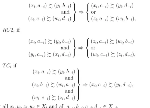
RC1i if (xi, a−i) % (yi, b−i) and (zi, c−i) % (wi, d−i) ⇒ (xi, c−i) % (yi, d−i) or (zi, a−i) % (wi, b−i), RC2i if (xi, a−i) % (yi, b−i) and (yi, c−i) % (xi, d−i) ⇒ (zi, a−i) % (wi, b−i) or (wi, c−i) % (zi, d−i), T Ci if (xi, a−i) % (yi, b−i) and (zi, b−i) % (wi, a−i) and (wi, c−i) % (zi, d−i) ⇒ (xi, c−i) % (yi, d−i),
for all xi, yi, zi, wi ∈ Xi and all a−i, b−i, c−i, d−i ∈ X−i.
We say that % satisfies RC1 (resp RC2, T C) if it satisfies RC1i (resp.
RC2i, T Ci) for all i ∈ N ; RC12 (resp. RC12i) is short for RC1 and RC2
Condition RC1i (inteR-attribute Cancellation) suggests that % induces
on X2
i a relation that compares “preference differences” in a well-behaved
way: if (xi, yi) is a “larger preference difference” than (zi, wi) and (zi, c−i) %
(wi, d−i) then we should have (xi, c−i) % (yi, d−i) and vice versa. This
rela-tion, which we denote by %∗
i, is formally defined as
(xi, yi) %∗i (zi, wi) iff
[for all c−i, d−i ∈ X−i, (zi, c−i) % (wi, d−i)⇒ (xi, c−i) % (yi, d−i)](12)
for all xi, yi, zi, wi ∈ Xi. Relation %∗i is transitive by construction and RC1i
exactly amounts to asking that it is complete, hence a weak order. The equivalence relation ∼∗
i defined in (8) is the symmetric part of %∗i.
Condition RC2i suggests that the “preference difference” (xi, yi) is linked
to the “opposite” preference difference (yi, xi). Again, RC1i and RC2i are
equivalent to requiring that the relation %∗∗
i , defined on Xi2 by
(xi, yi) %∗∗i (zi, wi) iff [(xi, yi) %i∗ (zi, wi) and (wi, zi) %∗i (yi, xi)], (13)
be complete (it is transitive by construction) and thus a weak order.
Condition T Ci (Triple Cancellation) is a classical cancellation condition
that has been often used in the analysis of the additive value model (see e.g. Wakker (1989) or Bouyssou and Pirlot (2002b), for interpretation).
No other condition is required in order to characterise models (M0), (M1), (M10), (M2), (M20), (M3) and (M30) as long as the sets X
i are finite or
denumerable. When the latter hypothesis is not fulfilled, restrictions must be imposed in order to ensure that either ∼∗
i, %∗i or %∗∗i have a numerical
representation. These will be needed also for the characterisation of the suffixed models. Property LCC ensures that each equivalence class of ∼± i
can be unambiguously identified by a real number (which is realised by the functions ui); we have seen in the proof of lemma 1 that this implies that
there are enough real numbers to label the equivalence classes of ∼∗ i; thus
LCC, that is necessary for guaranteeing the existence of the ui functions in
the D−suffixed models, can substitute the (weaker) hypothesis used in the characterisation of the initial models (condition C∗ in Bouyssou and Pirlot
(2002b)). The condition used for ensuring the representability of weak orders remains necessary. This condition can be formulated as follows.
We say that % satisfies OD∗
i if there is a finite or countably infinite
subset of X2
i that is dense in Xi2 for %∗i. In case %∗i is a weak order, OD∗i
function pi on Xi2 such that, for all (xi, yi), (zi, wi) ∈ Xi2, (xi, yi) %∗i (zi, wi)
iff pi(xi, yi) ≥ pi(zi, wi). Condition OD∗ is said to hold if condition OD∗i
holds for i = 1, 2, . . . , n. 3.2.3 Results
The theorem below describes all “–D” suffixed models listed in table 1. Theorem 1 Let % be a binary relation on a set X = Qn
i=1Xi. If X is at
most denumerable, then:
1. any binary relation % satisfies model (M– D),
2. % satisfies model (M0– D) iff % is reflexive and independent,
3. % satisfies model (M1– D) iff % satisfies model (M10– D) iff % is
re-flexive, independent and satisfies RC1,
4. % satisfies model (M2– D) iff % satisfies model (M20– D) iff % is
re-flexive and satisfies RC12,
5. % satisfies model (M3– D) iff % is complete and satisfies RC12, 6. % satisfies model (M30– D) iff % is complete and satisfies T C.
7. If X is not denumerable, parts 1 and 2 remain valid iff the requirement that % satisfies condition LCC is added; parts 3, 4, 5, 6 remain valid iff the requirement that % satisfies conditions LCC and OD∗ is added.
The above results constitute a straightforward adaptation of theorems 1 and 2 in Bouyssou and Pirlot (2002b) ; the characterisation of models (M) to (M30) extends immediately to that of the corresponding “M– D”
model if X is denumerable since we have seen that, in such a case, pi(xi, yi)
decomposes without further condition into ϕi(ui(xi), ui(yi)). Part 7 deserves
a word of explanation. Condition LCC obviously is necessary to guarantee the existence of ui in all models and OD∗ is necessary in all models in which
F is required to be at least nondecreasing (the latter was shown in Bouyssou and Pirlot (2002b, theorem 2)). It should be noted that condition LCC may not be dispensed of, even in the presence of OD∗, in part 7 of the theorem,
as shown by example 18 in appendix B. Bouyssou and Pirlot (2002b) showed that the conditions used in this theorem are independent.
3.3
Variants of intra- and inter-attribute
decompos-able models
Lemma 1 shows that imposing monotonicity properties on ϕi without
re-quirements on F does not lead to new models; in the same way, as we have seen in theorem 1, the conditions previously considered in model (M) and imported in model (M– D) without imposing monotonicity properties on ϕi
do not generate new models either (as long as the cardinality of Xi is not
strictly larger than that of R). It thus remains to examine—and this is the main goal of the present paper—the possible effect of properties imposed correlatively both on the “inter” and the “intra” components of the model.
For each of the eight models described in table 1, we consider two spe-cialisations in which property 1 (respectively 10) is imposed on the functions
ϕi. They are various instances of “nontransitive decomposable models” with
which the intra-attribute decomposability requirements combine without im-plying however the full force of additivity and subtractivity. These variants will be identified by replacing the suffix “– D” either by “– D1” or by “– D10”
depending on the fact that property 1 or 10 is respectively added. For each
model in table 1, we shall thus consider a version in which, for all i = 1, . . . , n, ϕi(ui(xi), ui(yi)) is nondecreasing in ui(xi) and nonincreasing in ui(yi)
(prop-erty 1) and a version in which it is increasing in ui(xi) and decreasing in ui(yi)
(property 10).
The – D1 or – D10 variants of model (M– D) have been analysed in section
3.1 and proven equivalent to the unconstrained model (M– D). The same is true for the – D1 or – D10 variants of model (M0– D) that are equivalent to
(M0– D1), because (M0) does not impose any monotonicity on F . We state this result in the following lemma; its proof—a slight modification of that of lemma 1—is relegated in Appendix A.1.
Lemma 2 A relation % on X satisfies model (M0– D1) or, equivalently, model (M0– D10) iff it is reflexive, independent and satisfies property LCC.
These conditions are independent. Remarks
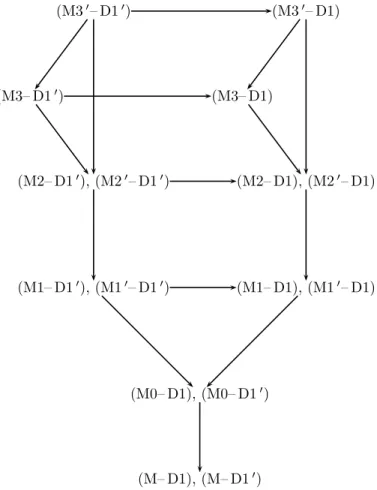
1. The preliminary study done so far leaves us with twelve models to analyse, namely, for k = 1, 2, 3, (Mk– D1), (Mk0– D1), (Mk– D10) and
(Mk0– D10). Some of these will turn out to be equivalent; their
Figure 1 shows the implications between those models ; for the sake of readability, only direct implications are drawn. Note that we have also:
• (Mk– D1) ⇒ (Mk) , for k = 1, 2, 3 ; • (Mk0– D1)⇒ (Mk0) , for k = 1, 2, 3 .
2. It is interesting to observe and easy to prove that the various proper-ties imposed on F , ϕi and ui in our models induce properties of the
marginal preferences %J, J ⊆ N , and links between %J and % that
become closer and closer to what is obtained with the additive value function model (2). For the reader’s convenience, we recall in the next proposition three consequences that were established in Bouyssou and Pirlot (2002b) and that we adapt to the “(M– D)” context . We add two new consequences that reveal possible effects of interaction between monotonicity conditions imposed both on F and ϕi.
Proposition 1 Let % be a binary relation on X =Qn
i=1Xi.
1. If % satisfies model (M1– D) or (M10– D) then:
[xi Âi yi, for all i∈ J ⊆ N ] ⇒ N ot[yJ %J xJ].
2. If % satisfies model (M2– D) or (M20– D) then:
• %i is complete,
• [xi Âi yi for all i∈ J ⊆ N ] ⇒ [xJ ÂJ yJ].
3. If % satisfies model (M30– D) then:
• [xi %i yi for all i∈ J ⊆ N ] ⇒ [xJ %J yJ],
• [xi %i yi for all i ∈ J ⊆ N, xj Âj yj, for some j ∈ J] ⇒ [xJ ÂJ
yJ].
4. If % satisfies model (M1– D1) then %i is a semi-order.
5. If % satisfies model (M30– D10) then %
(M30– D10) (M30– D1) (M3– D10) (M3– D1) (M20– D10) (M20– D1) (M2– D10) (M2– D1) (M10– D10) (M10– D1) (M1– D10) (M1– D1) (M0– D1) (M0– D10) (M– D1) (M– D10)
Proof of Proposition 1
For the proof of parts 1), 2) and 3), see Bouyssou and Pirlot (2002b, proposition 1).
4) We first prove that %i has the Ferrers property, i.e., if xi %i yi and
zi %i wi, then at least one of the following holds : zi %i yi or xi %i wi. From
the premise, using obvious notation, we get F (ϕi(ui(xi), ui(yi)), 0−i) ≥ 0
and F (ϕi(ui(zi), ui(wi)), 0−i)≥ 0. We have either ui(yi)≥ ui(wi) or ui(yi) <
ui(wi). In the former case, due to the monotonicity properties of F and
ϕi, we get F (ϕi(ui(xi), ui(wi)), 0−i) ≥ 0, hence xi %i wi; in the latter case,
F (ϕi(ui(zi), ui(yi)), 0−i) ≥ 0 and thus zi %i yi. The Ferrers property of %i
is thus established. It is well-known (and easy to prove) that the Ferrers property implies completeness provided the relation is reflexive, which is the case of %i in (M1– D1).
The semi-transitivity property results from showing, in a similar manner, that xi %i yi and yi %i zi entail either xi %i wi or wi %i zi, for any wi ∈ Xi.
5) Since we already know that %i is a semi-order, it remains to prove that
the marginal indifference ∼i is transitive. Due to the skew-symmetry of ϕi
and the increasingness of F in model (M30), it is readily seen that x
i ∼i yi if
and only if ϕi(ui(xi), ui(yi)) = 0. In model (M30– D10), since ϕi is decreasing
in its second argument and since ϕi(ui(xi), ui(xi)) = 0, we have xi ∼i yi if
and only if ui(xi) = ui(yi). From this, one clearly obtains that xi ∼i yi and
yi ∼i zi imply xi ∼i zi. 2
Remarks
1. Obviously, any property of %i, valid in a model, is inherited by any
of the more constrained model (see the implications between models in figure 1). In particular, the semi-order property (proposition 1.4) is valid in models (M2– D1) and (M3– D1).
2. Pure (M) models, without intra-attribute decomposability, confer lit-tle structure to the marginal preferences %i. It is only with (M2)
that %i becomes a complete relation. On the contrary, in the
intra-decomposable models, from (M1– D1) on, %i is a semi-order.
3. It is only in the more restrictive model (M30– D10) that %
i is a weak
order. In such a model, two elements of Xi that are marginally
indiffer-ent must have equal ui values, as results from the proof of proposition
4
Axioms
This section has two subsections. The first one states and proves an auxiliary result on relations defined on a Cartesian product of a set with itself. In the second subsection, we present the axioms that will help us to analyse the models introduced in section 3.2; we prove some elementary consequences of these axioms.
4.1
Properties of weak orders on X
i2In view of setting down the axioms that govern intra-attribute decompos-ability in our models, we first pay attention to the weak order %pi on X2
i
represented by the function pi(xi, yi) = ϕi(ui(xi), ui(yi)), i.e. (xi, yi) %pi
(zi, wi) ⇔ pi(xi, yi) ≥ pi(zi, wi). Note that pi need not be a numerical
rep-resentation of %∗
i or %∗∗i (it may be “finer”, see lemma 5 in section 5.2) and
hence, %pi
is not necessarily %∗
i or %∗∗i .
What will be of particular interest is linking properties of ϕi to those of
%pi. In order to reduce notational burden and since the following definitions
and results are fairly general and may be interesting in their own, we formu-late them in terms of a set A (instead of Xi) and a function f (instead of
pi).
To any binary relation %A defined on a cartesian product A2, can be
associated the relations E and T defined on A letting, for all a, b∈ A: aEb⇔ (a, c) ∼A (b, c) and (c, b)∼A(c, a), for all c∈ A (14)
and
aT b⇔ (a, c) %A (b, c) and (c, b) %A(c, a) for all c∈ A. (15) Relation T is usually called the trace of %A and E is the symmetric part of
T . Following mainly Monjardet (1984) and Doignon, Monjardet, Roubens, and Vincke (1988), we say that:
• %Ais strongly linear iff [N ot((b, c) %A(a, c)) or N ot ((c, a) %A(c, b))] ⇒
[(a, d) %A(b, d) and (d, b) %A(d, a)],
• %A is strongly independent iff [(a, c) %A (b, c)) or (c, b) %A (c, a))]⇒
[(a, d) %A(b, d) and (d, b) %A(d, a)],
for all a, b, c, d∈ A.
We note a few simple and useful observations in the following lemma (its proof is left to the reader).
Lemma 3 Let %A be a relation on A2, ∼A, its symmetric part, T , its trace
and E, the symmetric part of T . We have:
1. If ∼A is an equivalence, then E is an equivalence.
2. If %A is transitive, then T is transitive.
3. %A is strongly linear iff T is complete.
As an elementary consequence of these properties, we have that the trace T of a strongly linear weak order %A is a weak order.
The following result studies the situation in which %Ais a weak order
induced on A2 by a function f : A2 → R. The case where A is not
denu-merable raises technical problems of representability on the real numbers. In addition to the condition LCCi introduced in section 3.1 (the relation ∼±i
corresponds exactly to E), we need the classical order density condition (see section 2) to ensure that the trace T is representable on R.
Proposition 2 Let f : A2 → R and %fbe the weak order induced on A2 by
f , i.e. (a, b) %f (c, d) iff f (a, b)≥ f (c, d), for all a, b, c, d ∈ A.
1. %fis reversible iff there is a function f0 such that f0(a, b) = −f0(b, a)
and (a, b) %f (c, d) iff f0(a, b)≥ f0(c, d)
2. Suppose that A is at most denumerable. There are a function u : A→ R and a function ϕ : u(A)× u(A) → R such that f (a, b) = ϕ(u(a), u(b)). Furthermore,
(a) the function ϕ can be taken to be nondecreasing in its first argu-ment and nonincreasing in its second arguargu-ment iff %fis strongly
linear;
(b) the function ϕ can be taken to be increasing in its first argument and decreasing in its second argument iff %fis strongly
3. In case A is not a denumerable set, there exist a function u : A → R and a function ϕ : u(A)× u(A) → R such that f (a, b) = ϕ(u(a), u(b)) iff the number of equivalence classes of the relation E is not larger than the cardinality of R. Properties 2(a) and 2(b) hold iff there is a finite or denumerable subset of A that is dense in A for T .
Proof of Proposition 2
1) Sufficiency is obvious. We prove necessity. Suppose that %fis reversible.
Define f0(a, b) = f (a, b)− f (b, a); f0 obviously is skew-symmetric. We show
that f0provides another representation of %f. Since %fis reversible, we have
(a, b) %f (c, d) iff (d, c) %f (b, a). Hence, f (a, b) ≥ f (c, d) and f (d, c) ≥
f (b, a) and finally, f0(a, b) ≥ f0(c, d). Conversely, if f0(a, b) ≥ f0(c, d), we
have that f (a, b)≥ f (c, d). Suppose, on the contrary, that f (a, b) < f (c, d). Since f0(a, b) ≥ f0(c, d), it must be that f (b, a) < f (d, c) implying (d, c) %f
(b, a) and, since %fis reversible, (a, b) %f (c, d), a contradiction.
2) The existence of ui and ϕi has been established in section 3.1, around
(11); this proof transposes immediately for establishing the existence of u and ϕ (∼∗
i corresponds to ∼ and ∼±i to E).
Part 2)(a) [⇒]. Suppose that N ot [(b, c) %f (a, c)] or N ot [(c, a) %f (c, b)],
for some a, b, c ∈ A. This is equivalent to f (b, c) < f (a, c) or f (c, a) < f (c, b). Using the monotonicity properties of ϕ, we obtain from both inequalities that u(a) > u(b) and that ϕ(u(a), u(d)) ≥ ϕ(u(b), u(d)) and ϕ(u(d), u(b)) ≥ ϕ(u(d), u(a)), for all d ∈ A. This establishes that %fis strongly linear.
Part 2)(a) [⇐]. Since %f is a strongly linear weak order, T is a weak order
(Lemma 3, parts 2 and 3). Let u be a numerical representation of T , i.e. aT b iff u(a)≥ u(b); such a representation exists since A is finite or denumerable. Define ϕ by ϕ(u(a), u(b)) = f (a, b). ϕ is well-defined since u(c) = u(d) iff c(T ∩ T−1)d, i.e. cEd; the reasoning made just after formula (11) thus
holds. Moreover ϕ is nondecreasing in its fist argument and nonincreasing in the second. To prove the former, suppose that u(a) > u(b); this implies aT b. We have for all c ∈ A, (a, c) %f (b, c) and hence f (a, c) ≥ f (b, c).
Non-increasingness in the second argument is similarly proven.
Part 2)(b) [⇒]. Suppose, on the contrary, that %fis not strongly
indepen-dent. Among the four possible cases, we have, for instance, that (a, c) %f
(b, c) and N ot [(a, d) %f (b, d)], for some a, b, c, d ∈ A. This is tantamount to
ϕ(u(a), u(c)) ≥ ϕ(u(b), u(c)) and ϕ(u(a), u(d)) < ϕ(u(b), u(d)), which im-ply respectively, due to increasingness of ϕ in its first argument, u(a)≥ u(b) and u(a) < u(b), a contradiction. The other cases can be dealt with similarly.
Part 2)(b) [⇐]. We define u and ϕ as in part 2)(a). Let a, b ∈ A be such that u(a) > u(b). Since u is a numerical representation of T , we have aT b and N ot [bT a]; strong independence implies that, for all c ∈ A, N ot [(b, c) %f
(a, c)] and N ot [(c, a) %f (c, b)], i.e. f (a, c) > f (b, c) and f (c, b) > f (c, a).
Suppose, for instance, that ϕ is not increasing in its first argument. This would imply that, for some a, b, d∈ A, with u(a) > u(b), f (a, d) ≤ f (b, d), a contradiction. A similar argument proves that ϕ is decreasing in its second argument.
3) In case A is not denumerable, the condition on E is clearly necessary and sufficient for being able to represent each equivalence class of that relation by a real number. The order density condition makes it possible to consider a numerical representation of the weak order T by means of a real-valued function u; this condition is thus sufficient. To show it is also necessary, it suffices to observe that any function u in a representation of %fwith ϕ
monotonic is a representation of a weak order that is at least as fine as T . In other words, if aT b and N ot [bT a], u(a) > u(b). 2 Remarks
1. Proposition 2 reformulates in our framework classical results that may essentially be found in Doignon et al. (1988), Tversky and Russo (1969) (see also Pirlot and Vincke (1997) for a synthesis). Take any numerical representation of %A. This representation may be seen as a valued
relation on A2. In the terminology of Doignon et al. (1988, section 4.4),
the valued relation obtained when %A is strongly linear is a coherently
biordered valued relation. The families of binary relations obtained by considering all the cuts of these valued relations have been well studied (Doignon et al., 1988). To our knowledge the valued relations obtained when replacing linearity by independence have received no particular name in the literature.
2. Doignon et al. (1988) distinguish three less restrictive versions of lin-earity, namely, left-linlin-earity, right-linearity and linearity. We do not investigate these notions for the sake of conciseness; the reader should note that distinguishing left and right linearity (or independence) has strong connections with a slightly more general model where pi(xi, yi)
is decomposed as ϕi(ui(xi), vi(yi)) with ui not necessarily equal to vi.
3. The results in Doignon et al. (1988) are expressed for finite sets. They extend, at least those we consider, to denumerable sets, without further condition. In view of obtaining the results in section 5.3 below, we need further extension to non-denumerable sets and we obtain it under rather straightforward necessary and sufficient conditions, as shown in part 3 of proposition 2.
4. It is important to note that in case f has particular features—for in-stance if f vanishes on the diagonal (f (a, a) = 0, for all a) or f is skew-symmetric—these are inherited by ϕ. This will be of importance in our models when f = pi and %fpossibly is the relation %∗i or the
relation %∗∗
i .
4.2
Axioms for intra-criteria decomposability
In view of proposition 2.2 and 2.3, and the construction of numerical represen-tations for models of type (M) (see Bouyssou and Pirlot (2002b)), obtaining intra-decomposable models boils down to imposing linearity conditions on %∗i
and %∗∗
i . In order to do so, we introduce a number of intrA-attribute
Can-cellation (AC) conditions and of Triple intrA-attribute CanCan-cellation (TAC) conditions. We say that % satisfies:
AC1i if (xi, a−i) % y and (zi, c−i) % w ⇒ (zi, a−i) % y or (xi, c−i) % w, AC2i if x % (yi, b−i) and z % (wi, d−i) ⇒ x % (wi, b−i) or z % (yi, d−i), AC3i if (xi, a−i) % y) and z % (xi, d−i) ⇒ (wi, a−i) % y) or z % (wi, d−i)
for all x, y, z, w ∈ X and all a−i, b−i, c−i, d−i ∈ X−i.
We say that % satisfies AC1 (resp AC2, AC3) if it satisfies AC1i (resp
as a short form for the conjunction of conditions AC1, AC2 and AC3 (resp. AC1i, AC2i and AC3i).
Condition AC1i suggests that the elements of Xi can be linearly
or-dered considering “upward dominance”: if xi “upward dominates” zi then
(zi, c−i) % w entails (xi, c−i) % w . Condition AC2i has a similar
interpreta-tion considering now “downward dominance”. More formally, let %+i (resp. %−i ) denote the left (resp. right) trace induced by % on Xi, i.e.
xi %+i zi iff ∀ c−i ∈ X−i, w ∈ X, [(zi, c−i) % w ⇒ (xi, c−i) % w] (16)
yi %−i wi iff ∀ a−i ∈ X−i, z ∈ X, [(yi, a−i) % z ⇒ (wi, a−i) % z] (17)
It was shown in Bouyssou and Pirlot (2002a, lemma 3) that AC1i (resp.
AC2i) is equivalent to imposing that %+i (resp. %−i ) is a complete relation,
hence a weak order (since it is transitive by definition).
Condition AC3iensures that the linear arrangements of the elements of Xi
obtained considering upward and downward dominance are not incompatible. In other terms, the trace %±i that is the intersection of %+i and %−i , i.e.
xi %±i zi iff [xi %i+ zi and xi %−i zi], (18)
is also a complete relation, hence a weak order.
It is also quite important to note that %±i is also the trace of %∗
i and %∗∗i
(defined by formulae (12) and (13)). Indeed, we can easily check that we have :
xi %±i yi iff ∀zi ∈ Xi, (xi, zi) %∗i (yi, zi)
and ∀wi ∈ Xi, (wi, yi) %∗i (wi, xi) (19)
The latter expression implies that %±i is the trace both of %∗
i and %∗∗i .
Re-mark that the relation ∼±i , defined in (9), is the symmetric part of %±i .
The Triple intrA-attribute Cancellation (TAC) conditions read as follows. We say that % satisfies
TAC1i if (xi, a−i) % y and y % (zi, a−i) and (zi, b−i) % w ⇒ (xi, b−i) % w
TAC2i if (xi, a−i) % y and y % (zi, a−i) and w % (xi, b−i) ⇒ w % (zi, b−i)
for all y, w ∈ X, all xi, zi ∈ Xi and all a−i, b−i ∈ X−i.
We say that % satisfies TAC1 (resp TAC2) if it satisfies TAC1i (resp
TAC2i), for i = 1, 2, . . . , n. We shall also use TAC12 (resp. TAC12i) for the
conjunction of conditions TAC1 and TAC2 (resp. TAC1i and TAC2i).
The TAC1i, TAC2i conditions are variants of the classical triple
cancella-tion condicancella-tion, like T Ci in section 3.2. As soon as % is complete, TAC1 and
TAC2 become powerful conditions (as was the case of T C in models (M)) that imply AC123; they will help to make sure, in certain models, that ties can be broken just by using “upward” or “downward dominance”.
The above axioms and their consequences have been studied in detail in Bouyssou and Pirlot (2002a). The following lemma recalls results that will be needed in the sequel and establishes new ones showing that some of the axioms are intimately related to strong linearity of %∗
i and %∗∗i .
Lemma 4 We have:
1. Model (M1– D1) implies AC123. 2. Model (M30– D10) implies TAC12.
3. %+i is complete iff AC1i holds
4. %−i is complete iff AC2i holds
5. %±i is complete iff AC123i holds
6. AC123i ⇔ %∗i is strongly linear ⇔ %∗∗i is strongly linear.
7. If % is complete, TAC12i ⇒ AC123i and if one of the alternatives
in the consequent of any of AC1i, AC2i or AC3i is false, then the
8. If % is complete, TAC1i is equivalent to the completeness of %+i and
the following condition:
[x % y and zi Â+i xi]⇒ (zi, x−i)Â y. (20)
9. If % is complete, TAC2i is equivalent to the completeness of %−i and
the following condition:
[x % y and yi Â−i wi]⇒ x  (wi, y−i). (21)
Proof of Lemma 4
1) The premise of AC1i yields in terms of model (M1– D1):
F (ϕi(ui(xi), ui(yi)), (ϕj(uj(aj), uj(yj)))j6=i)≥ 0
and
F (ϕi(ui(zi), ui(wi)), (ϕj(uj(cj), uj(wj)))j6=i)≥ 0.
Due to the monotonicity of F and ϕi, either ui(zi)≥ ui(xi) and
F (ϕi(ui(zi), ui(yi)), (ϕj(uj(aj), uj(yj)))j6=i))≥ 0,
or ui(xi) > ui(zi) and
F (ϕi(ui(xi), ui(wi)), (ϕj(uj(cj), uj(wj)))j6=i)≥ 0,
which implies that AC1i is satisfied. The proof for AC2iand AC3i is similar.
2) The premise of TAC1i, interpreted in terms of model (M30– D10), yields
three inequalities :
F (ϕi(ui(xi), ui(yi)), (ϕj(uj(aj), uj(yj)))j6=i) ≥ 0 (22)
F (ϕi(ui(yi), ui(zi)), (ϕj(uj(yj), uj(aj)))j6=i) ≥ 0 (23)
F (ϕi(ui(zi), ui(wi)), (ϕj(uj(bj), uj(wj)))j6=i) ≥ 0. (24)
Due to skew-symmetry of ϕi and oddness of F , equation (23) may be
rewrit-ten as :
We deduce from equations (22) and (25), using the increasingness of F (resp. ϕi) in its ith (resp. first) argument, that ui(xi) ≥ ui(zi); substituting ui(zi)
by ui(xi) in equation (24) yields :
F (ϕi(ui(xi), ui(wi)), (ϕj(uj(bj), uj(wj)))j6=i)≥ 0,
which establishes TAC1i. The proof for TAC2i is similar.
Parts 3), 4) and 5) were respectively proven as lemma 3, parts 1, 2 and 4 in Bouyssou and Pirlot (2002a).
6) Using (19), we observed above that %±i is not only the trace of % but also of both %∗
i and %∗∗i . Applying lemma 3.3, with A = Xi and %A=%∗i or
%∗∗
i , we get that %∗i and %∗∗i are strongly linear iff %±i is complete, which, in
turn, is equivalent to AC123i (by part 5) of the present lemma).
7) We prove that, if % is complete, TAC1iimplies AC1iand AC3i. Suppose
that AC1i is violated so that (xi, a−i) % y, (zi, b−i) % w, N ot[(zi, a−i) % y]
and N ot[(xi, b−i) % w], for some xi, zi ∈ Xi, a−i, b−i ∈ X−i and y, w ∈ X.
Since % is complete, we know that y % (zi, a−i). Using TAC1i, (xi, a−i) % y,
y % (zi, a−i) and (zi, b−i) % w imply (xi, b−i) % w, a contradiction.
Similarly, suppose that AC3i is violated so that (xi, a−i) % y, w %
(xi, b−i), N ot[(zi, a−i) % y] and N ot[w % (zi, b−i)], for some xi, zi ∈ Xi,
a−i, b−i ∈ X−i and y, w∈ X. Since % is complete, we have: (zi, b−i) % w.
Us-ing TAC1i, (zi, b−i) % w, w % (xi, b−i) and (xi, a−i) % y imply (zi, a−i) % y,
a contradiction.
One proves similarly that TAC2i implies AC2i and AC3i.
For proving the second part of the thesis, we need using TAC1i (resp.
TAC2i) for the statement concerned with AC1i(resp. AC2i) and both TAC1i
and TAC2ifor the statement concerned with AC3i. Let us prove the result for
AC1i(the proof is similar in the two other cases). Suppose that the premise of
AC1i is verified, i.e. (xi, a−i) % y and (zi, c−i) % w, while the first alternative
of the consequent is false, i.e. N ot [(zi, a−i) % y]; suppose eventually that the
second branch of the alternative is not a strict preference, which means that (xi, c−i) ∼ w. Applying TAC1i to the premise [(zi, c−i) % w, w % (xi, c−i)
and (xi, a−i) % y] yields (zi, a−i) % y, a contradiction. If, on the contrary,
the second branch of the alternative is false, i.e. N ot [(xi, c−i) % w], and
supposing that the first branch of the alternative is (zi, a−i) ∼ y, we get,
applying TAC1i to [(xi, a−i) % y, y % (zi, a−i) and (zi, c−i) % w ], the fact
Parts 8) and 9) were respectively shown as lemma 4, parts 4 and 5 in Bou-yssou and Pirlot (2002a).
2
5
Results
We are now in a position to provide a characterization of all intra- and inter- decomposable models defined in section 3.3, using in particular the “AC” and “TAC” conditions introduced in the previous section. For ease of reading and in order to concentrate first on the core arguments, we start with the case where the Xi’s are at most denumerable, postponing to subsection
5.3 below, the technicalities inherent to sets of arbitrary cardinality. In the denumerable case, we deal separately (respectively in subsections 5.1 and 5.2) with the “– D1” and the “– D10” models, finally showing that all pairs
of models differing only by – D1 or – D10 are equivalent except for (M30– D1)
and (M30– D10). For the sake of completeness, we include in our theorems,
results about models (M– D1), (M– D10), (M0– D1) and (M0– D10) that were
already included in lemmas 1 and 2.
5.1
Non strictly monotonic decomposable models in
the denumerable case
In the next theorem, we consider the models studied in theorem 1, with the additional property that they admit a representation in which ϕi is
nonde-creasing in its first argument and noninnonde-creasing in the second. It is remark-able that this property is obtained for all models (except for M and M0) as soon as conditions AC123 are added to the axioms stated in theorem 1. Theorem 2 Let % be a binary relation on a finite or countably infinite set X =Qn
i=1Xi. Then:
1. % satisfies model (M– D1);
2. % satisfies model (M0– D1) iff % is reflexive and independent;
3. % satisfies model (M10– D1) iff % is reflexive, independent and
4. % satisfies model (M20– D1) iff % is reflexive and satisfies RC12 and
AC123;
5. % satisfies model (M3– D1) iff % is complete and satisfies RC12 and AC123;
6. % satisfies model (M30– D1) iff % is complete and satisfies T C and
AC123.
Proof of theorem 2
Parts 1) and 2) are consequences of lemmas 1 and 2. For all parts from 3) to 6), necessity results from theorem 1 and lemma 4.1. It remains to prove sufficiency.
3) We have to recall how a reflexive, independent relation satisfying RC1 can be represented in model (M10). Detailed justification of such a
construc-tion can be found in Bouyssou and Pirlot (2002b). Due to RC1, %∗
i is a weak
order on X2
i; since Xi2 is denumerable, we may choose for pi : Xi2 −→ R, a
numerical representation of %∗
i. Since % is independent, we have (xi, xi)∼∗i
(yi, yi), for all xi, yi ∈ Xi; we may thus impose that pi(xi, xi) = 0 for all
xi ∈ Xi. We then define F for instance as :
F (p1(x1, y1), p2(x2, y2), . . . , pn(xn, yn)) = (26) ½ exp(Pn i=1pi(xi, yi)) if x % y, − exp(−Pn i=1pi(xi, yi)) otherwise. Under AC123, %∗
i is strongly linear (lemma 4.6) ; by proposition 2.2, there
are functions ui and ϕi such that the numerical representation pi of %∗i may
be written as pi(xi, yi) = ϕi(ui(xi), ui(yi)) with ϕi nondecreasing in its first
argument and nonincreasing in the second.
4) The construction of F for a relation that satisfies model (M20) is almost
the same; the only difference lies in the fact that we may choose pi a
nu-merical representation of the weak order %∗∗
i (instead of %∗i) and in addition
impose that pi(xi, yi) = −pi(yi, xi) (skew-symmetry). The skew-symmetric
pi functions may then be decomposed as in the previous case since by lemma
4, part 6, %∗∗
i is strongly linear.
5) and 6) For models (M3) and (M30), which are distinct, we have to modify
slightly the definition of F . Take for pi a skew-symmetric numerical
repre-sentation of %∗∗
i , like in model (M20), and define F as follows:
exp(Pn i=1pi(xi, yi)) if x y, 0 if x∼ y, − exp(−Pn i=1pi(xi, yi)) otherwise.
F again is well-defined (see Bouyssou and Pirlot (2002b) for details); it is odd in view of the definition of F and the fact that the relation % is complete. In model (M3), F is nondecreasing in all pi but not necessarily strictly
increas-ing; in this model we may not exclude indeed that x∼ y, (zi, wi)Â∗∗i (xi, yi)
and (zi, x−i)∼ (wi, y−i), for some x, y∈ X and zi, wi ∈ Xi. In model (M30),
when axiom T C is in force, such a situation never occurs and, with the same construction, F is strictly increasing. Due to lemma 4, part 6, %∗∗
i is strongly
linear and in both models, pi may thus be decomposed as in case 3).
2 5.1.1 Equivalence of models and independence of axioms
The equivalence of two pairs of models directly results from theorem 2 and the previous results. We note them in the following corollary.
Corollary 1 If X is at most denumerable,
1. models (M1– D1) and (M10– D1) are equivalent;
2. models (M2– D1) and (M20– D1) are equivalent.
The proof is immediate since by theorem 1 and lemma 4.1, the weaker model (M1– D1) (resp. (M2– D1)) satisfies all the properties that characterize the stronger (M10– D1) (resp. (M20– D1)), according to theorem 2.
In appendix B we provide examples showing that none of the axioms char-acterizing the models described in theorem 2, parts 3 to 6 is a consequence of the others (for part 1 there is nothing to prove and proving the indepen-dence of the axioms for part 2 is left to the reader). Table 2 summarizes the properties of the examples 1 to 8 in appendix B. The non-redundancy of the properties used for characterizing the various models in theorem 2 is established
• for part 3, by examples 1, 6, 8, 3, 4, 5;
• for part 6, by examples 1, 2, 3, 4, 5.
The order in which the examples are listed corresponds to the order in which the properties characterizing the models appear in parts 3 to 6 of theorem 2: for each model, each example violates the corresponding property in the characterization of the model while it satisfies all the others.
Table 2: Properties of Examples 1 to 8 in Appendix B R C RC1 RC2 I TC AC1 AC2 AC3 Ex1 0 0 1 1 1 1 1 1 1 Ex2 1 1 1 1 1 0 1 1 1 Ex3 1 1 1 1 1 1 0 1 1 Ex4 1 1 1 1 1 1 1 0 1 Ex5 1 1 1 1 1 1 1 1 0 Ex6 1 1 1 0 0 0 1 1 1 Ex7 1 1 1 0 1 0 1 1 1 Ex8 1 1 0 1 1 0 1 1 1
Meaning of the abbreviations: “R” for “reflexive”; “C” for “complete”; “I” for “independent”.
5.2
Strictly monotonic decomposable models in the
denumerable case
In this section we extend our analysis to “strictly monotonically” decompos-able models, i.e. we deal with all models suffixed by −D10.
Theorem 3 Let % be a binary relation on a finite or countably infinite set X =Qn
i=1Xi. Then:
1. parts 1, 2, 3, 4 and 5 of theorem 2 remain true when D1 is substituted by D10 in the labels of the models;
2. % satisfies model (M30– D10) iff % is complete and satisfies T C and
TAC12.
Except for the first two models (corresponding to parts 1 and 2 of theorem 2, which have been proved in lemmas 1 and 2 respectively), the proof of theorem
3 is rather technical. It develops the following idea. For each of the models characterized in theorem 2, with the exception of the sixth one, we show that the functions ϕi that appear in the representation and are nondecreasing in
their first argument and nonincreasing in their second, can be substituted by functions that are strictly increasing in their first argument and strictly decreasing in their second. The proof of the theorem relies on lemmas 5 and 6 stated below; the proof of these lemmas is deferred to appendix A.2 and A.3.
Since we are planning to transform the functions ϕi that appear in the
representation of % in our models, we need knowing how much freedom we have for doing so. It is important to keep in mind that the functions pi
appearing in the various (Mk ) and (Mk0) models need not be a numerical
representation of %∗
i (in model (M1) or (M10)) or of %∗∗i (in models (M2),
(M20), (M3) or (M30)). Our first lemma states the precise (necessary and
sufficient) conditions that pi has to fulfill in the numerical representations of
the various models.
Lemma 5 1. Let % satisfy model (M1) or (M10). A function p
i : Xi2 →
R, with pi(xi, xi) = 0, for all xi ∈ Xi, can be used in a representation
of % according to model (M1) or (M10) iff
(zi, wi)Â∗i (xi, yi)⇒ pi(zi, wi) > pi(xi, yi). (28)
2. Let % satisfy model (M2), (M20) or (M3). A function p
i : Xi2 →
R, with pi(xi, yi) = −pi(yi, xi), for all xi, yi ∈ Xi, can be used in a
representation of % according to model (M2), (M20) or (M3) iff
(zi, wi)Â∗∗i (xi, yi)⇒ pi(zi, wi) > pi(xi, yi). (29)
3. Let % satisfy model (M30). A function p
i : Xi2 → R, with pi(xi, yi) =
−pi(yi, xi), for all xi, yi ∈ Xi, can be used in a representation of %
according to model (M30) iff
(zi, wi)Â∗∗i (xi, yi)⇒ pi(zi, wi) > pi(xi, yi).
and
(zi, wi)∼∗∗i (xi, yi) and
∃ a−i, b−i ∈ X−i s.t. (xi, a−i)∼ (yi, b−i)
¾
⇒ pi(zi, wi) = pi(xi, yi).
The next lemma states, in a fairly general framework, the conditions under which a function ϕ of two variables that is nondecreasing in its first argument and nonincreasing in the second can be transformed into a strictly monotonic function ψ. Consider a function ϕ : U × U → R, with U, a subset of R, and suppose that ϕ is nondecreasing in its first argument and nonincreasing in the second. There are two types of situations that may cause the lack of strict monotonicity of ϕ ; we denote by S, the set of values r of ϕ for which either there are a, b, c∈ U such that :
ϕ(a, c) = ϕ(b, c) = r with a > b (31) or there are a, c, d∈ U such that :
ϕ(a, c) = ϕ(a, d) = r with c > d. (32) Clearly, ϕ is strictly monotonic iff S is empty. The role played by the set S is crucial as we can see in the next lemma.
Lemma 6 Let U be a subset of the ]0, 1[ interval and ϕ : U × U → R that vanishes on the diagonal (ϕ(u, u) = 0, for all u ∈ U) and is nondecreasing in its first argument and nonincreasing in the second.
1. If S is at most denumerable, there exists a function ψ : U × U → R that vanishes on the diagonal, is increasing in its first argument and decreasing in the second and satisfies the following properties: for all u, v, u0, v0 ∈ U,
[ϕ(u, v) > ϕ(u0, v0)]⇒ [ψ(u, v)) > ψ(u0, v0)]. (33) and
[ϕ(u, v) = ϕ(u0, v0)]⇒ [ψ(u, v)) = ψ(u0, v0)] iff ϕ(u, v) 6∈ S (34)
If, in addition, ϕ is skew-symmetric, there exists a skew-symmetric ψ with the same properties as above.
2. If S is not denumerable, there is no function ψ that is increasing in its first argument, decreasing in the second and satisfies (33).