EMPIRICAL MEANS TO VALIDATE SKILLS MODELS AND ASSESS THE FIT OF A STUDENT MODEL
BEHZAD BEHESHTI
DÉPARTEMENT DE GÉNIE INFORMATIQUE ET GÉNIE LOGICIEL ÉCOLE POLYTECHNIQUE DE MONTRÉAL
THÈSE PRÉSENTÉE EN VUE DE L’OBTENTION DU DIPLÔME DE PHILOSOPHIÆ DOCTOR
(GÉNIE INFORMATIQUE) AVRIL 2016
c
ÉCOLE POLYTECHNIQUE DE MONTRÉAL
Cette thèse intitulée :
EMPIRICAL MEANS TO VALIDATE SKILLS MODELS AND ASSESS THE FIT OF A STUDENT MODEL
présentée par : BEHESHTI Behzad
en vue de l’obtention du diplôme de : Philosophiæ Doctor a été dûment acceptée par le jury d’examen constitué de :
M. GUÉHÉNEUC Yann-Gaël, Doctorat, président
M. DESMARAIS Michel C., Ph. D., membre et directeur de recherche M. GAGNON Michel, Ph. D., membre
DEDICATION
ACKNOWLEDGEMENTS
I would like to express my deepest gratitude to my advisor Michel C. Desmarais who has provided constant guidance and encouragement throughout my research at Ecole Polytechnique de Montreal. I do not know where my research would go without his patience and efforts.
I would like to thank administrative staff and system administrators in the department of Computer En-gineering at Ecole Polytechnique de Montreal for their incredible helps.
At the end, words cannot express how grateful I am to my family who never stopped supporting me even from distance. A special thanks to my friends who always inspire me to strive towards my goals.
RÉSUMÉ
Dans le domaine de l’analytique des données éducationnelles, ou dans le domaine de l’apprentissage automatique en général, un analyste qui souhaite construire un modèle de classification ou de régression avec un ensemble de données est confronté à un très grand nombre de choix. Les techniques d’apprentis-sage automatique offrent de nos jours la possibilité de créer des modèles d’une complexité toujours plus grande grâce à de nouvelles techniques d’apprentissage. Parallèlement à ces nouvelles possibilités vient la question abordée dans cette thèse : comment décider lesquels des modèles sont plus représentatifs de la réalité sous-jacente ?
La pratique courante est de construire différents modèles et d’utiliser celui qui offre la meilleure pré-diction comme le meilleur modèle. Toutefois, la performance du modèle varie généralement avec des facteurs tels que la taille de l’échantillon, la distribution de la variable ciblée, l’entropie des prédicteurs, le bruit, les valeurs manquantes, etc. Par exemple, la capacité d’adaptation d’un modèle au bruit et sa ca-pacité à faire face à la petite taille de l’échantillon peut donner de meilleures performances que le modèle sous-jacent pour un ensemble de données.
Par conséquent, le meilleur modèle peut ne pas être le plus représentatif de la réalité, mais peut être le résultat de facteurs contextuels qui rendent celui-ci meilleur que le modèle sous-jacent.
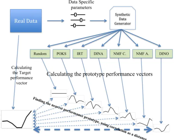
Nous étudions la question de l’évaluation de modèles différents à partir de données synthétiques en définissant un espace vectoriel des performances de ceux-ci, et nous utilisons une l’approche du plus proches voisins avec une distance de corrélation pour identifier le modèle sous-jacent. Cette approche est basée sur les définitions et les procédures suivantes. Soit un ensemble de modèles,M , et un vecteur p de longueur |M | qui contient la performance de chaque modèle sur un ensemble de données. Ce vecteur représente un point qui caractérise l’ensemble de données dans l’espace de performance. Pour chaque modèle M dans M , nous déterminons un point pi dans l’espace de performance qui correspond à des
données synthétiques générées par le modèle Mi. Puis, pour un ensemble de données, nous trouvons le
point pi le plus proche, en utilisant la corrélation comme distance, et considérons le modèle Mi l’ayant
généré comme le modèle sous-jacent.
Les résultats montrent que, pour les ensembles de données synthétiques, leurs ensembles de modèles sous-jacents sont généralement plus souvent correctement identifiés par l’approche proposée plutôt que par le modèle avec la meilleure performance. Ils montrent aussi que les modèles sémantiquement simi-laires sont également plus rapprochés dans l’espace de performance que les modèles qui sont basés sur des concepts très différents.
ABSTRACT
In educational data mining, or in data mining in general, analysts that wish to build a classification or a regression model over new and unknown data are faced with a very wide span of choices. Machine learning techniques nowadays offer the possibility to learn and train a large and an ever growing variety of models from data. Along with this increased display of models that can be defined and trained from data, comes the question addressed in this thesis: how to decide which are the most representative of the underlying ground truth?
The standard practice is to train different models, and consider the one with the highest predictive per-formance as the best fit. However, model perper-formance typically varies along factors such as sample size, target variable and predictor entropy, noise, missing values, etc. For example, a model’s resilience to noise and ability to deal with small sample size may yield better performance than the ground truth model for a given data set.
Therefore, the best performer may not be the model that is most representative of the ground truth, but instead it may be the result of contextual factors that make this model outperform the ground truth one. We investigate the question of assessing different model fits using synthetic data by defining a vector space of model performances, and use a nearest neighbor approach with a correlation distance to identify the ground truth model. This approach is based on the following definitions and procedure. Consider a set of models,M , and a vector p of length |M | that contains the performance of each model over a given data set. This vector represents a point that characterizes the data set in the performance space. For each model M ∈M , we determine a new point in the performance space that corresponds to synthetic data generated with model M. Then, for a given data set, we find the nearest synthetic data set point, using correlation as a distance, and consider the model behind it to be the ground truth.
The results show that, for synthetic data sets, their underlying model sets are generally more often cor-rectly identified with the proposed approach than by using the best performer approach. They also show that semantically similar models are also closer together in the performance space than the models that are based on highly different concepts.
TABLE OF CONTENTS
DEDICATION . . . iii
ACKNOWLEDGEMENTS . . . iv
RÉSUMÉ . . . v
ABSTRACT . . . vi
TABLE OF CONTENTS . . . vii
LIST OF TABLES . . . x
LIST OF FIGURES . . . xi
LIST OF ABBREVIATIONS . . . xii
CHAPTER 1 INTRODUCTION . . . 1
1.1 Problem Definition and Challenges . . . 1
1.1.1 Model selection and goodness of fit . . . 1
1.2 Thesis vocabulary . . . 2 1.3 Research Questions . . . 4 1.4 General Objectives . . . 4 1.5 Hypotheses . . . 4 1.6 Main Contributions . . . 5 1.7 Publications . . . 5
1.8 Organization of the Thesis . . . 6
CHAPTER 2 STUDENT MODELLING METHODS . . . 7
2.1 Definitions and concepts . . . 7
2.1.1 Test outcome data . . . 7
2.1.2 Skills . . . 7
2.1.3 Q-matrix and Skill mastery matrices . . . 8
2.1.4 Types of Q-matrices . . . 8
2.2 Skills assessment and item outcome prediction techniques . . . 9
2.3 Zero skill techniques . . . 11
2.3.1 Knowledge Spaces and Partial Order Knowledge Structures (POKS) . . . 11
2.4.1 IRT . . . 13
2.4.2 Baseline Expected Prediction . . . 14
2.5 Multi-skills techniques . . . 14
2.5.1 Types of Q-matrix (examples) . . . 15
2.5.2 Non-Negative Matrix Factorization (NMF) . . . 16
2.5.3 Deterministic Input Noisy And/Or (DINA/DINO) . . . 19
2.6 Recent improvements . . . 19
2.6.1 NMF on single skill and multi-skill conjunctive Q-matrix . . . 20
2.6.2 Finding the number of latent skills . . . 20
2.6.3 The refinement of a Q-matrix . . . 21
2.7 Model selection and goodness of fit . . . 21
2.7.1 Measures for goodness of fit . . . 21
2.8 Related works . . . 23
2.8.1 On the faithfulness of simulated student performance data . . . 24
2.8.2 Simulated data to reveal the proximity of a model to reality . . . 26
CHAPTER 3 PERFORMANCE SIGNATURE APPROACH . . . 28
3.1 Model fit in a vector space framework . . . 29
3.2 Research questions . . . 30
3.2.1 Experiment 1: Predictive performance of models over real and synthetic datasets 31 3.2.2 Experiment 2: Sensitivity of the Model performance over different data genera-tion parameters . . . 33
3.2.3 Experiment 3: Model selection based on performance vector classification . . . 33
3.2.4 Experiment 4: Signature vs. best performer classification . . . 34
CHAPTER 4 SYNTHETIC DATA GENERATION . . . 35
4.1 Data generation parameters . . . 35
4.1.1 Assessing parameters . . . 35
4.2 POKS . . . 36
4.2.1 Obtaining parameters . . . 36
4.2.2 Data generation . . . 39
4.2.3 Data specific parameters . . . 39
4.3 IRT . . . 40
4.3.1 Generating parameters randomly . . . 40
4.3.2 IRT synthetic data process . . . 41
4.4 Linear models . . . 41
4.4.1 Q-matrix . . . 42
4.4.3 Synthetic data . . . 45
4.4.4 Noise factor . . . 45
4.5 Cognitive Diagnosis Models . . . 45
4.5.1 Skill space . . . 46
4.5.2 Skill distribution . . . 46
4.5.3 Slip and Guess . . . 46
4.6 Educational data generator . . . 47
CHAPTER 5 EXPERIMENTAL RESULTS . . . 49
5.1 Datasets . . . 49
5.2 Results of Experiment 1: Predictive performance of models over real and synthetic datasets 51 5.2.1 Discussion . . . 53
5.3 Results of Experiment 2: Sensitivity of the Model performance over different data gen-eration parameters . . . 54
5.3.1 Results and discussion . . . 54
5.4 Results of Experiment 3: Model selection based on performance vector classification . . 58
5.4.1 Results . . . 59
5.5 Results of Experiment 4: Nearest neighbor vs. best performer classification . . . 60
CHAPTER 6 CONCLUSION AND FUTURE WORKS . . . 63
6.1 Limitations . . . 64
6.2 Future Work . . . 64
LIST OF TABLES
Table 3.1 Vector space of accuracy performances . . . 29
Table 3.2 Parameters of the predictive performance framework . . . 32
Table 4.1 Parameters involved in synthetic data generation . . . 36
Table 5.1 Datasets . . . 50
Table 5.2 Parameters of the simulation framework . . . 54
Table 5.3 Degree of similarity between six synthetic datasets based on the correlation . . . 60
Table 5.4 Degree of similarity between six synthetic datasets and the ground truth based on the correlation . . . 60
Table 5.5 Confusion matrix for classification of 210 synthetic datasets on 7 models with Best performer Vs. Nearest neighbor methods . . . 61
LIST OF FIGURES
Figure 2.1 Four items and their corresponding Q-matrix . . . 9
Figure 2.2 Skills assessment methods . . . 10
Figure 2.3 Partial Order Structure of 4 items . . . 11
Figure 2.4 Oriented incidence matrix and Adjacency matrix . . . 12
Figure 2.5 An example for Conjunctive model of Q-matrix . . . 15
Figure 2.6 An example for Additive model of Q-matrix . . . 15
Figure 2.7 An example for Disjunctive model of Q-matrix . . . 16
Figure 3.1 Signature framework . . . 28
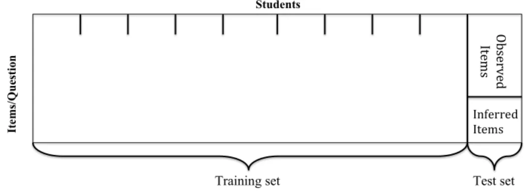
Figure 3.2 Data breakdown of cross validation process . . . 31
Figure 4.1 An example of random KS with 5 items . . . 38
Figure 4.2 Q-matrix and an example of simulated data with this matrix. Pale cells represent 1’s and red ones represent 0’s. . . 43
Figure 4.3 Additive model of Q-matrix and Corresponding synthetic data . . . 44
Figure 4.4 hierarchical structure of parameters of linear conjunctive model . . . 48
Figure 5.1 Two types of representation of predictive performance of 7 models over DINA generated dataset . . . 51
Figure 5.2 Item outcome prediction accuracy results of synthetic datasets . . . 52
Figure 5.3 Item outcome prediction accuracy results of real datasets. Note that the y-scale is different than the synthetic dataset. . . 52
Figure 5.4 Variation of Sample Size Over synthetic datasets . . . 55
Figure 5.5 Variation of Number of items Over synthetic datasets . . . 56
Figure 5.6 Variation of Number of skills Over synthetic datasets . . . 56
Figure 5.7 Variation of Item Variance Over synthetic datasets . . . 57
Figure 5.8 Variation of Student variance Over synthetic datasets . . . 57
Figure 5.9 Variation of Success Rate Over synthetic datasets . . . 58
LIST OF ABBREVIATIONS
NMF Non-negative Matrix Factorization POKS Partial Order Knowledge Structure IRT Item Response Theory
DINA Deterministic Input Noisy And DINO Deterministic Input Noisy Or SVD Singular Value Decomposition ALS Alternate Least-Square Factorization E-M Expectation–Maximization
MCMC Markov chain Monte Carlo RMSE Root Mean Square Error SSE Sum Square Error
CHAPTER 1 INTRODUCTION
1.1 Problem Definition and Challenges
In Educational Data Mining, or in Data Science in general, analysts that wish to build a classification or regression model over new and unknown data are faced with a very wide span of choices. Machine learning techniques nowadays offer the possibility to learn and train a large and an ever growing variety of models from data. Learning techniques such as the EM algorithm and MCMC methods have contributed to this expansion of models we can learn from data. In some cases, they allow model parameters esti-mation that would otherwise represent an intractable problem using standard analytical or optimization techniques.
Along with this increased display of models that can be defined and trained from data, comes the ques-tion of deciding which are the most representative of the underlying ground truth. This quesques-tion is of interest from two perspectives. One is the theoretical and explanatory value of uncovering a model that accounts for observed data. The other perspective is the assumption that the “true” underlying model will better generalize to samples other than the training data. This assumption is commonly supported in physics where some models have a window in the parameter space where they correctly account for observations, and break down outside that window; Newtownian and modern physics are prototypical examples supporting this assumption.
In the machine learning field, the case for the support of the assumption that the closer to the ground truth a model is, the better it will generalize outside the parameter space, is not as evident as it can be in physics. But we do find analogous examples such as the Naïve Bayes classifier under a 0-1 loss function tend to perform very well in spite of the unrealistic assumption of the naïve independence assumption at the root of the approach’s name (Domingos and Pazzani, 1997).
Given that in machine learning, we are often more interested in the predictive power of models than we are in their theoretical and explanatory value, the standard practice is to choose the model with the best predictive performance. And without good theoretical understanding of the domain, we simply hope that it will generalize outside the space covered by our training sample.
This thesis aims to provide a means to assess the fit of the model to the underlying ground truth using a methodology based on synthetic data, and to verify if the approach is better able to identify a model that will generalize outside the parameter space of the training sample. The study is circumscribed to the domain of Educational Data Mining where we find numerous competing models of student skills mastery.
1.1.1 Model selection and goodness of fit
Model selection is the task of selecting a statistical model for a given data from a set of candidate models. Selection is most often based on a model’s “goodness of fit”.
On the other hand the term “goodness of fit” for a statistical model describes how well it fits a set of observation. The distance between observed values and the predicted values under the model can be a measure of goodness of fit. The goodness of fit is usually determined using likelihood ratio. There exist different approaches to assess model fit based on the measure of goodness of fit. The consensus is that the model with the best predictive performance is the most likely to be the closest to the ground Truth. Then there are the issues of how sensitive is the model to sample size, noise, and biases that also need to be addressed before we can trust that this model is the best candidate. It can take numerous studies before a true consensus emerges as to which model is the best candidate for a given type of data.
Another approach to assess which model is closest to the ground truth is proposed in this thesis. It relies on the analysis of model predictive performances over real data and synthetic data. Using synthetic data allows us to validate the sensitivity of the model selection approach to data specific parameters such as sample size and noise. Comparing performance over synthetic and real data has been used extensively to validate models, but we further elaborate on the standard principle of comparison over both types of data by contrasting the predictive performance across synthetic datasets with different types of underlying model. The hypothesis we make is that the relative performance of different models will be stable by the characteristic of a given type of data, as defined by the underlying ground truth for real data, or by the model that generates the synthetic data. We explore this hypothesis in the domain of Educational Data Mining and the assessment of student skills, where latent skills are mapped to question items and students skill mastery is inferred from item outcome results from test data. More specifically, this thesis focuses on static student skill models where we assume student skill mastery is stationary, as opposed to dynamic models where the time dimension is involved and where a learning process occurs.
The theoretical intuition behind this research is that the comparison of model performances to identify the ground truth provides a more powerful means than focusing on the individual model performances. This idea will be tested on synthetic data with predefined model parameter and consequently a predefined ground truth.
This chapter introduces and defines these concepts, as well as outlines the objectives and main scientific hypotheses of the proposed research. The final section presents the organization of the remainder of this research.
1.2 Thesis vocabulary
In this section we introduce a vocabulary that is related to the general objective of this thesis and used in all chapters:
— Student model: "In general terms, student modeling involves the construction of a qualitative rep-resentation that accounts for student behavior in terms of existing background knowledge about a domain and about students learning the domain. Such a representation, called a student model" (Sison and Shimura, 1998). Student skills assessment models are essentially constructed to assess student’s skills or estimate potential skills required for problems. Since our experiments are in
the domain of educational data mining, by the term “Model” we mean “student model”.
— Dataset (Real/Synthetic): Dataset in this context represents student test outcome which is a matrix that shows the result of a test given by students. A test is simply a set of few questions, problems or items that can have a success of a failure result in the dataset. Datasets can be “real” or “synthetic”. A “Real” dataset is the result of an actual test of n items given to m individuals in an e-learning environment or even a classroom. The term “Synthetic” means that a simulation is involved to generate an artificial student test outcome. The simulation is designed based on a model that takes a set of predefined parameters to generate student test outcome. This set has two types of parameters: Model specific parameters and Data specific parameters.
— Model specific parameters: These parameters are specifically defined and learnt based on model’s type. Complex models contain more parameters. Some models may share some parameters but some models have no parameters in common.
— Data specific parameters: These parameters are common between all datasets which are also known as “Contextual parameters” such as average success rate, sample size and number of items in a dataset.
— Ground truth: This term is originally coined by Geographical/earth science where if a location method such as GPS estimates a location coordinates of a spot on earth, then the actual location on earth would be the “Ground truth”. This term has been adopted in other fields of study. In this context “ground truth of a dataset” means the actual model that best describes the dataset within its parameters. Note that for the skills models studied here, the ground truth is always unknown, unless we use synthetic data.
— Performance of a model: The accuracy of a model to predict student response outcomes over a dataset (using cross-validation) is called performance of a model. Different models have different performances over a dataset. Assessing such a performance requires designing an experiment to learn the model’s parameters and predict a proportion of the dataset that has not been involved in the learning phase.
— Performance vector: Each model has a performance over a dataset. Consider a set of models,M , and a vector p of length |M | that contains the performance of each model over a given dataset. This vector represents a point in the performance space, and it is defined as the performance vectorof that dataset.
— Performance Signature: The performance vector can be considered from two perspectives: The first perspective is a performance vector in the performance space where we have the same number of dimensions as the number of candidate models in this vector. The second one is a kind of performance signaturefor a specific dataset that is used for the purpose of easier visualization in a single dimensional space. The performance vector is plotted as a line where each value of the vector is on the y scale and it creates a kind of “signature”. These terms are described in details along with examples later in section 5.2.
vectorassociated with the synthetic data of a model class. Note that there are different ways to produce the synthetic data of a model and we return to this question later.
— Target Performance Vector: This term is used to refer to the performance vector of the dataset with an unknown ground thruth that is to be classified into one of the candidate ground truth, each ground thruth corresponding to one the candidate models.
1.3 Research Questions
The following questions are addressed in this thesis:
1. What is the performance vector of student skills assessment models over real and over synthetic data created using the same models?
2. Is the performance vector unique to each synthetic data type (data from the same ground truth model)?
3. Can the performance vector be used to define a method to reliably identify the ground truth behind the synthetic data?
4. How does the method compare with the standard practice of using the model with the best perfor-mance?
1.4 General Objectives
The general objective of this thesis is to assess the goodness of fit on the basis of what we will refer to as performance signatures. It can be divided in three sub-objectives: The first objective is to obtain the performance signatures of skills assessment models over synthetic datasets generated with these very same models. This will create a vector of performances in the performance space. The second one is to assess model fit using the performance vector of the synthetic and real data. The third objective is to test the uniqueness and sensitivity of the performance vectors on the different data specific conditions such as sample size, nose, average success rate.
1.5 Hypotheses
The research in this thesis tests the following hypotheses:
Hypothesis 1: The performance vectors of two datasets with the same ground truth have a high level of correlation across different data specific parameters.
Hypothesis 2: The best performer model is not necessarily the ground truth model.
Hypothesis 3: Datasets with the same model parameters and data specific parameters create unique performance vector.
1.6 Main Contributions
The main contribution of this thesis is assessing model fit of a dataset by comparing its performance vectorto the performance prototype of synthetic datasets generated with the same data specific parame-ters of the given dataset but different skills assessment models. This method can be applied to different fields of studies but in this research we focus on student test result and on a few skills assessment models that have emerged mostly in EDM and ITS. The predictive performance of each model is assessed by designing an experiment, which learns the model parameters and observes a set of items for a student to predict the rest of items test results of that student. The mean predictive accuracy will be the pre-dictive performance measure. Previous researches compared their prepre-dictive performance on a pairwise basis, but few studies have taken a comprehensive approach to compare them on a common basis. In this research we used seven skills assessment models to obtain the predictive performance vector using the same models. The result of our experiment shows that synthetic datasets have discriminant pattern of performance vector across models. The capacity of recognizing a dataset’s true model relies on this discriminant characteristic.
The next step is to use this performance vector to assess model fit for a real dataset. The standard practice is to pick the “best performer” as the ground truth model. The actual best fitting model may have been overlooked due to an unfortunate estimate of the algorithm’s parameters. Therefore, the best performer may not be the model that is most representative of the ground truth, but instead it may be the result of contextual factors that make this model outperform the ground truth one. We investigate the question of assessing different model fits using synthetic data by defining a vector space based on model performances, and use a nearest neighbor approach on the bases of correlation to identify the ground truth model. Comparing the performance of synthetic dataset with a specific underlying model and the performance of a real dataset with the same underlying model should show a high correlation. Our investigations on synthetic data confirms that performance vectors from the same model generated datasets show high correlations among themselves.
Still the question of sensitivity of the performance signature to contextual factors should be considered in the comparison of the performance vectors. The other contribution is to test the stability of the “per-formance signature” of synthetic datasets over different data specific parameters (such as sample size, average success rate, etc.) generated with the same underlying model. Also our experiments shows that the performance vectors are stable across different data parameters. In other words, the cloud of points for a particular model (Ground truth) with different data specific parameter values which is not too dispersed.
1.7 Publications
Along the course of the doctorate studies, I contributed to a number of publications, some of which are directly related to this thesis, and some of which are peripheral or are preliminary studies that led to the thesis.
1. B. Beheshti, M.C. Desmarais, “Assessing Model Fit With Synthetic vs. Real Data" , Journal Submitted to Journal of Educational Data Mining.
2. B. Beheshti, M.C. Desmarais, “Goodness of Fit of Skills Assessment Approaches: Insights from Patterns of Real vs. Synthetic Data Sets", Short Paper in International Educational Data Min-ing 2015 June 2015, Madrid, Spain, pp: 368-371.
3. B. Beheshti, M.C. Desmarais, R. Naceur, “Methods to Find the Number of Latent Skills”, short paper in International Educational Data Mining 2012 July 2012, Crete, Greece. , pp: 81-86. 4. B. Beheshti, M.C. Desmarais, “Improving matrix factorization techniques of student test data
with partial order constraints", Doctoral consortium in User Modeling, Adaptation, and Per-sonalization 2012 Aug 2012, Montreal, Canada. , pp: 346-350.
5. M.C. Desmarais, B. Beheshti, P. Xu, “The refinement of a q-matrix: assessing methods to validate tasks to skills mapping", Short paper in International Educational Data Mining 2014 June 2014, London, United Kingdom., pp: 308-3011.
6. M.C. Desmarais, B. Beheshti, R. Naceur, “Item to skills mapping: deriving a conjunctive q-matrix from data”, short paper in Intelligent Tutoring Systems 2012 July 2012, Crete, Greece. , pp: 454-463.
7. M.C. Desmarais, P. Xu, B. Beheshti, “Combining techniques to refine item to skills Q-matrices with a partition tree", Full Paper in International Educational Data Mining 2015 June 2015, Madrid, Spain., pp: 29-36.
8. M.C. Desmarais, R. Naceur, B. Beheshti, “Linear models of student skills for static data", Work-shop in User Modeling, Adaptation, and Personalization 2012 July 2012, Montreal, Canada. 1.8 Organization of the Thesis
We review the related literature on fundamental concepts in Educational Data Mining and some ma-chine learning techniques that have been used in our experiments in Chapter 2. Chapter 2 also discusses recent work about model selection. The main contribution of the research starts from chapter 3 where we explain the proposed approach in details. As a complementary part of the proposed approach we explain synthetic data generation approaches in chapter 4. The experimental results of the main contribution are explained in details in Chapter 5. Finally, we conclude and outline future work in Chapter 6.
CHAPTER 2 STUDENT MODELLING METHODS
A large body of methods have been developed for student modeling. They are used to represent and assess student skills and they are a fundamental part of intelligent learning environments (Desmarais and Baker, 2011). These models have been proposed both for dynamic performance data, where a time dimension is involved and where a learning process occurs (see for eg. Bayesian Knowledge Tracing in Koedinger et al. (2011)), and for static performance data where we assume student skill mastery is stationary. In this thesis, we focus on static performance data.
We assume that skills explain the performance and test outcome prediction. Student models incorporate single or multiple skills. Some even model performance without explicit skills and we will refer to them as zero-skill models. The most widely used one is Item Response Theory (IRT). In its simplest version, IRT considers a single skill for student performance data. Of course, sometimes there are many skills involve in a single problem and therefore this model becomes insufficient for many applications in Intelligent Tutoring Systems (ITS). Under certain conditions, multi-skills models can perform better in that case. Other methods, such as POKS, have no latent skills. They just look at the relation between those items that are directly observable among test outcome items. The details of each category of techniques along with some examples are described in the next section.
2.1 Definitions and concepts
In this section some concepts and basic definitions that are common between most of student models are described.
2.1.1 Test outcome data
The student test outcome data, or more simply student test data, can consist in results from exams or from exercises, in the context of an e-learning environment or in paper and pencil form. We use the term itemto represent exercises, questions, or any task where the student has to apply a skilled performance to accomplish. Student answers are evaluated and categorized as success (1) or failure (0). The data represents a snapshot of the mastery of a student for a given subject matter, as we assume that the student’s knowledge state has not changed from the time of answer to the first question item to the last one. Test data is defined as an m × n matrix, R. It is composed of m row items and n column students. If a student successfully answers an item, the corresponding value in the results matrix is 1, otherwise it is 0. 2.1.2 Skills
In this thesis we consider skills as problem solving abilities. For example in mathematics “addition”, “division” are typical skills. They can also be further detailed, such as single digit and multi-digit addi-tion. There may be a single skill required to solve a problem or multiple skills. Skills are termed latent
because they are never observed directly.
If an item requires multiple skills, there are three different ways in which each skill can contribute to succeed a problem: The first case is when mastering a skill is mandatory for a student to succeed an item that requires it. The second case is when the skill increases the chance to succeed a problem. The third case is when at least one of the skills from the set of skills for an item is required to succeed that item. We will see later that the temrs conjunctive, compensatory/additive, and disjunctive are often used to refer to each case respectively.
Skills can have different range of values based on the student model definition. For example, the single skill in IRT is continuous in R and typically ranges between −4 to +4. Some student models consider skills range between 0 and 1. Finally, other models have binary 1 or 0 skills, which means it can be mastered or not. Details of definition of skills for each student model are given later in this chapter. 2.1.3 Q-matrix and Skill mastery matrices
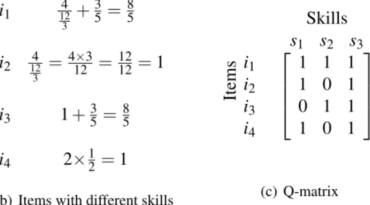
Curriculum design can be a complex task and an expert blind spots in designing curricula is possible. It is desirable to have an alternative to human sequenced curricula. To do so, there should be a model designed for this purpose which maps skills to items (Tatsuoka, 1983, 2009). Figure 2.1 shows an example of this mapping which is named Q-matrix. Figure 2.1(b) shows 4 items and each item requires different skills (or combination of skills) to be successfully answered. Assuming 3 skills such as fraction multiplication (s1), fraction addition (s2) and fraction reduction (s3), these questions can be mapped to skills like the
Q-matrix represented in figure 2.1(c).
Such a mapping is desirable and very important in student modeling; because optimal order of problems (sequence of repetition and presentation) can be determined by this model since it allows prediction of which item will cause learning of skills that transfer to the other items most efficiently. It can also be used to assess student knowledge of each concept, and to personalize the tutoring process according to what the student knows or does not know. For example, Heffernan et al. in (Feng et al., 2009) have developed an intelligent tutoring system (the ASSISTment system) that relies on fine grain skills mapped to items. Barnes, Bitzer, & Vouk in (Barnes et al., 2005) were among the early researchers to propose algorithms for automatically discovering a Q-Matrix from data. In some context there is a constraint for the number of latent skills which is: k < nm/(n + m) (Lee et al., 1999) where k , n and m are number of skills, students and items respectively.
The skills mastery matrix, S, represents student skills mastery profiles. In this matrix rows are skills and columns represent examinees. A cell with the value of 1 in Si j indicates that examinee j is proficient in
skill i and a value of 0 shows that he does not have the related skill. 2.1.4 Types of Q-matrices
As explained earlier, skills can have three interpretations when they contribute to succeed an item. These interpretations can be reflected in Q-matrices. There exists three different types of Q-matrices which are useful based on the context of a problem domain:
s1: fraction multiplication s2: fraction addition s3: fraction reduction (a) Skills i1 124 3 +35 =85 i2 124 3 =4×312 = 1212 = 1 i3 1 +35= 85 i4 2×12 = 1
(b) Items with different skills
Skills s1 s2 s3 Items i1 i2 i3 i4 1 1 1 1 0 1 0 1 1 1 0 1 (c) Q-matrix
Figure 2.1 Four items and their corresponding Q-matrix
— Conjunctive: The most common one is the conjunctive model of the Q-matrix which is the standard interpretation of the Q-matrix in Educational Data Mining. In this type, a student should master all the required skills by an item to succeed it. If a student misses any one of these skills, then the result will be a failure in the test outcome data. Thus there is a conjunction between required skills.
— Additive (compensatory): Compensatory or additive model of skills is an interpretation of a Q-matrix where each skill contributes some weight to succeed that item. For example, if an item requires two skills a and b with the same weight for each of them, then each skill will contribute equally to yield a success of the item. In the compensatory model of Q-matrix, each skill increases the chance of success based on its weight.
— Disjunctive: In the disjunctive model, mastery of any single skill required by an item is sufficient in order to succeed the related item.
Note that in practice these types of interpretations becomes reasonable when there is at least one item in the Q-matrix that requires more than one skill otherwise they preform the same as each other. Later in this chapter these types will be described in more details with examples.
Q-matrices can also be categorized according to the number of skills per item:
— Single skill per item: Each item should have exactly one skill but the Q-matrix can have many skills.
— Multiple skills per item: Any combination of skills with at least one skill is possible for items. 2.2 Skills assessment and item outcome prediction techniques
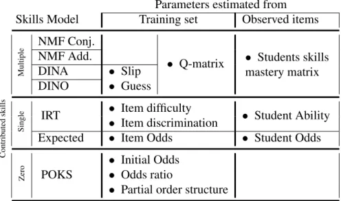
The skills assessment models we compare can be grouped into four categories: (1) the Knowledge Space frameworks which models a knowledge state as a set of observable items without explicit reference to latent skills, (2) the single skill Item Response Theory (IRT) approach, (3) the matrix factorization approach, which decomposes the student results matrix into a Q-matrix that maps items to skills, and a skills matrix that maps skill to students, and which relies on standard matrix algebra for parameter
estimation and item outcome prediction, and finally (4) the DINA/DINO approaches which also refer to a Q-matrix, but incorporate slip and guess factors and rely on different parameter estimation techniques than the matrix factorization method. We focus here on the assessment of static skills, where we assume the test data represents a snapshot in time, as opposed to models that allow the representation of skills that change in time, which is more typical of data from learning environments (see Desmarais and Baker (2012), for a review of both approaches).
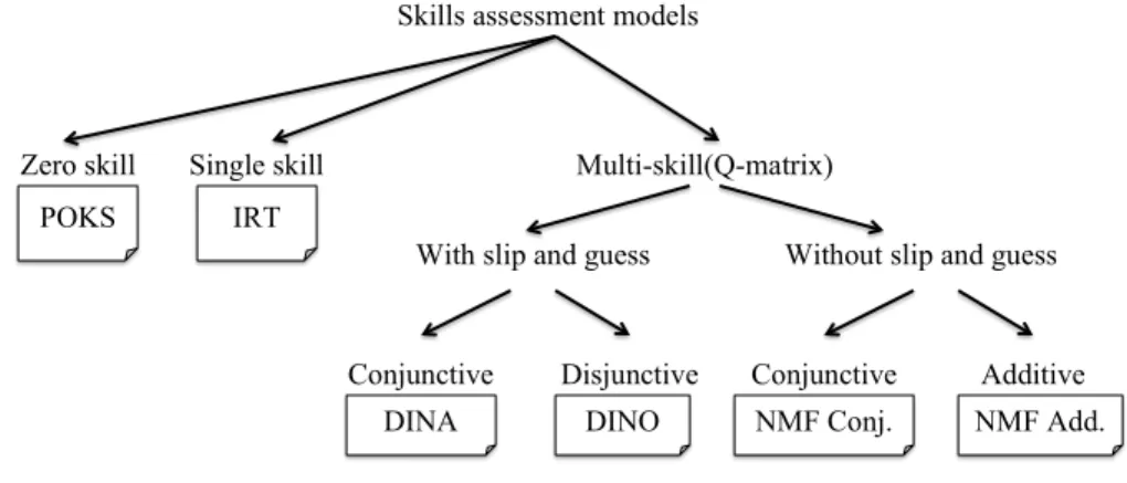
The skills assessment model we compare can be classified at a first level according to whether they model skills directly, and whether they are single or multiple skills. Then, multi-skills model can be further broken down based on whether they have guess and slip parameters, and whether the skills are considered disjunctive or conjunctive. Figure 2.2 shows this hierarchy of models.
Skills assessment models
Zero skill Single skill Multi-skill(Q-matrix)
POKS IRT
With slip and guess Without slip and guess
Conjunctive Disjunctive
DINA DINO
Conjunctive Additive NMF Add. NMF Conj.
Figure 2.2 Skills assessment methods
Considering these techniques from the perspective of variety of skills in test outcome prediction, we can put them in the following categories:
— Zero skill technique that predict item outcome based on observed items. POKS is the technique that is used from this category.
— Single skill approaches, where every item is linked to the same single skill. Item Response Theory (IRT) is the typical representative of this approach, but we also use the “expected value” approach which, akin to IRT, incorporates estimates of a the student’s general skill and the item difficulty to yield a predicted item outcome.
— Multi-Skills techniques that rely on Q-matrices to predict test outcome. Deterministic Input Noisy And/Or (DINA/DINO), NMF Conjunctive and Non-negative Matrix Factorization (NMF) addi-tive are the techniques we use in this study.
Note that the “expected value” approach is also considered as a baseline for our evaluations. The details of the different approaches are described below.
2.3 Zero skill techniques
Zero skill techniquesare so called because they make no explicit reference to latent skills. They are based on the Knowledge Space theory of Doignon and Falmagne (Doignon and Falmagne, 1999; Desmarais et al., 2006), which does not directly attempt to model underlying skills but instead rely on observable items only. An individual’s knowledge state is represented as a subset of these items. In place of rep-resenting skills mastery directly, they leave the skills assessment to be based on the set of observed and predicted item outcomes which can be done in a subsequent phase. TETRAD (Scheines et al., 1998) is a software that identifies pre-requisite relationships among items which is widely used in EDM.
POKS is one of the models adopted in our study that is a derivative of Knowledge Space Theory. POKS stands for Partial Order Knowledge Structures. It is a more constrained version of Knowledge Spaces theory (Desmarais et al., 1996a). POKS assumes that items are learned in a strict partial order. It uses this order to infer that the success to hard items increases the probability of success to easier ones, or conversely, that the failure to easy items decreases the chances of success to harder ones.
2.3.1 Knowledge Spaces and Partial Order Knowledge Structures (POKS)
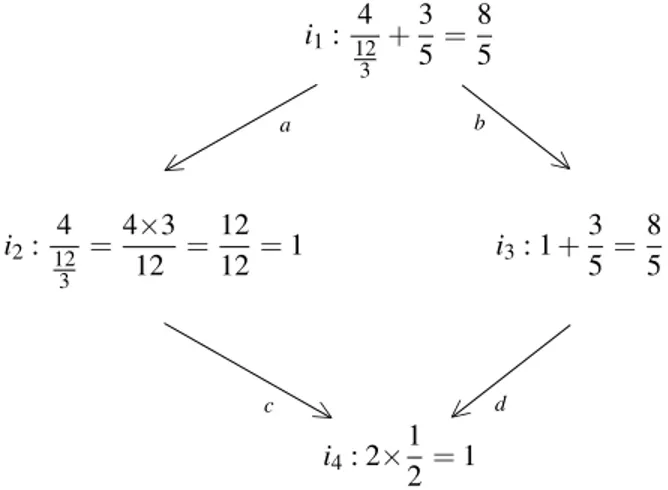
Items are generally learnt in a given order. Children learn easy problems first, then harder problems. It reflects the order of learning a set of items in the same problem domain. POKS learns the order structure from test data in a probabilistic framework. For example in figure 5.3 four items are shown in a partial order of knowledge structure. It is required for an examinee to be able to answer i4in order to solve i3
and i2. Also for solving i1, one should be able to answer i2, i3 and i4. if an examinee was not able to
answer i4then he would have less chance to answer correctly other items.
i1: 4 12 3 +3 5 = 8 5 a < b > i2: 4 12 3 =4×3 12 = 12 12= 1 i3: 1 + 3 5= 8 5 i4: 2× 1 2 = 1 d < c >
Figure 2.3 Partial Order Structure of 4 items
This is reflected in the results matrix R by closure constraints on the possible knowledge states. Defining a student knowledge state as a subset of all items (i.e. a column vector in R), then the space of valid knowledge states is closed under union and intersection according to the theory of Knowledge spaces
(Doignon and Falmagne, 1985). In POKS, this constraint is relaxed to a closure under union, meaning that the union of any two individual knowledge states is also a valid knowledge state. This means that the constraints can be expressed as a partial order of implications among items, termed a Partial Or-der Knowledge Structure (POKS). The algorithm to Or-derive such structures from the data in R relies on statistical tests (Desmarais et al., 1996b; Desmarais and Pu, 2005).
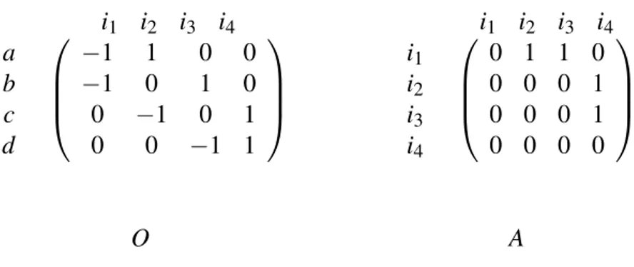
A knowledge structure can be represented by an Oriented incidence matrix, O, or by an Adjacency matrix, A. In the oriented incidence matrix, rows are edges and columns are nodes of the graph. The value of -1 shows the start node of an edge and 1 indicates the end of an edge. Therefore for each row (edge) there is only one pair of (-1,1) and the rest of cells are 0. In adjacency matrix both rows and columns are Items and if there is a link between a pair of items (for example i → j) there should be a 1 in Ai j otherwise it
is 0. Figure 2.4 shows the corresponding oriented incidence matrix and adjacency matrix of the structure in figure 5.3. i1 i2 i3 i4 a b c d −1 1 0 0 −1 0 1 0 0 −1 0 1 0 0 −1 1 i1 i2 i3 i4 i1 i2 i3 i4 0 1 1 0 0 0 0 1 0 0 0 1 0 0 0 0 O A
Figure 2.4 Oriented incidence matrix and Adjacency matrix
The structure of the partial order of items is obtained from a statistical hypothesis test that reckons the existence of a link between two items, say A → B, on the basis of two Binomial statistical tests P(B|A) > α1and P(¬A|¬B) > α1and under a predetermined alpha error of an interaction test (α2). The
χ2 test is often used, or the Fisher exact test. The values of α1= .85 and α2= .10 are chosen in this
study across all experiments.
A student knowledge state is represented as a vector of probabilities, one per item. Probabilities are updated under a Naive Bayes assumption as simple posterior probabilities given observed items.
Inference in the POKS framework to calculate the node’s probability relies on standard Bayesian poste-riors under the local independence assumption. The probability update for node H given E1,... Encan be
written in following posterior odds form:
O(H|E1, E2, ..., En) = O(H) n
∏
i P(Ei|H) P(Ei|H) (2.1)where odds definition is O(H|E) = 1−P(H|E)P(H|E) . If evidence Ei is negative for observation i, then the ratio P(Ei|H)
2.4 Single skill approaches
Other approaches incorporate a single latent skill in the model. This is obviously a strong simplification of the reality of skilled performance, but in practice it is a valid approximation as results show. When a model uses single latent skill, in fact it projects all the skills mastery level in a form of uni-dimensional representation that implicitly combines all skills. Then there would be a single continuous skill variable which is a weighted average of the skills mastery levels of an examinee.
In this section two approaches for modeling static test data are presented: the well established Item Response Theory (IRT), which models the relationship between observation and skill variable based on a logistic regression framework. It dates back to the 1960’s and is still one of the prevailing approaches (Baker and Kim, 2004). The second approach is a trivial approach we call Expected Prediction. This approach is also used as a baseline in our experiments.
2.4.1 IRT
The IRT family is based on a logistic regression framework. It models a single latent skill (although variants exists for modeling multiple skills) (Baker and Kim, 2004). Each item has a difficulty and a discrimination parameter.
IRT assumes the probability of success to an item Xjby student i is a function of a single ability factor θi:
P(Xj= 1 | θi) =
1 1 + e−aj(θi−bj)
In the two parameter form above, referred to as IRT-2pl, where parameters are: aj represents the item discrimination;
bj represents the item difficulty, and
θi the ability of a single student.
Student ability, θi, is estimated by maximizing the likelihood of the observed response outcomes
proba-bilities:
P(X1, X2, ..., Xj, θi) =
∏
jP(Xj|θi)
This corresponds to the usual logistic regression procedure. Note that the 2PL version of IRT is equivalent to the 3PL model with c parameter equal to zero which represents pseudo guessing.
A simpler version of IRT called the Rash model, fixes the discrimination parameter, a, to 1. Fixing this parameter reduces overfitting, as the discrimination can sometimes take unrealistically large values. Rash model is a valid model for student skills modeling, but we do use the more general IRT-2pl model, which includes both a and b, for the synthetic data generation process in order to make this data more realistic (chapter 4 discusses data generation approaches in details).
2.4.2 Baseline Expected Prediction
As a baseline model, we use the expected value of success to item i by student j, as defined by a product of odds:
O(Xi j) = O(Xi)O(Sj)
where O(Xi) is the odds of success to item i by all participants and O(Sj) is the odds of success rate of
student j. Both odds can be estimated from a sample. Recall that the transformation of odds to probability is P(X ) = 1/(1 + O(X )), and conversely O(X ) = P(X )/(1 − P(X )). Probabilities are estimated using the Laplace correction: P(X ) = ( f (x = 1) + 1)/( f (x = 1) + f (x = 0) + 2), where f (x = {1, 0}) represents the frequency of the corresponding category x = 1 or x = 0.
2.5 Multi-skills techniques
Finally the last category of student skills assessment models are considering student test result with multiple latent skills. Representation of multiple skills is possible in the form of a Q-matrix where skills are mapped to each item. As explained before, there exist different types of Q-matrices that each type represents a unique interpretation. The following sections will describe different skills assessment models along with their specific type of Q-matrix.
Still this category of models can be divided into two sub-categories:
— Models that infer a Q-matrix from test result data, such as models that uses matrix factorization techniques.
— Models that require a predefined Q-matrix to predict test outcome. These techniques can not directly infer the Q-matrix but they can refine an existing expert-defined Q-matrix.
Deriving a matrix from a test result matrix is challenging. Some models require a pre-defined Q-matrix. In some cases an expert defined Q-matrix is available but minor mistakes in mapping skills to items are always possible even by an expert. The basic challenge is to derive a perfect Q-matrix out of a test result matrix to give it as an input parameter to some models. This challenge also creates other challenges such as optimum number of latent skills for a set of items in a test outcome. Sometimes there exist more than single Q-matrix associated with a test result with different number of skills. Finding the optimum number of skills to derive a Q-matrix is a question that is given in more details in section 2.6.2. Given the number of latent skills, there exist few techniques to derive a Q-matrix for models that require one. Cen et al. (Cen et al., 2005, 2006) have used Learning Factor Analysis(LFA) technique to improve the initially hand-built Q-matrix which maps fine-grained skills to questions. They used log data which is based on the fact that the knowledge state of student dynamically changes over time as the student learns. In the case of static data of student knowledge, Barnes (Barnes, 2006) developed a method for this mapping which works based on a measure of the fit of a potential Q-matrix to the data. It was shown to be successful as well as Principal Component Analysis for skill clustering analysis. In our experiment we use NMF as a technique to derive a Q-matrix given an optimum number of latent skills. Later in this section we will introduce NMF in more details. Section 2.6.1 describes how to derive a conjunctive
model of Q-matrix from a student test result.
For real datasets there exists few expert defined Q-matrices. To use them as an input parameter for student skills assessment models we need to refine them. Section 2.6.3 gives few approaches to this problem. 2.5.1 Types of Q-matrix (examples)
As mentioned before, there are three models for the Q-matrix which are useful based on the context of the problem domain. The most important one is the conjunctive model of the Q-matrix, which is the standard interpretation of the Q-matrix. In figure 5.2 an example of conjunctive model of Q-matrix is shown. Examinee e1 answered item i1 and item i4 because he has mastered in the required skills but
although he has skill s1he couldn’t answer item i3which requires skill s2as well.
Examinee e1 e2 e3 e4 Items i1 i2 i3 i4 1 0 1 0 0 1 0 0 0 0 1 0 1 0 0 0 Skills s1 s2 s3 Items i1 i2 i3 i4 1 0 0 0 1 1 1 1 0 1 0 1 Examinees e1 e2 e3 e4 Skills s1 s2 s3 1 0 1 0 0 1 1 1 1 1 0 0 R Q S
Figure 2.5 An example for Conjunctive model of Q-matrix
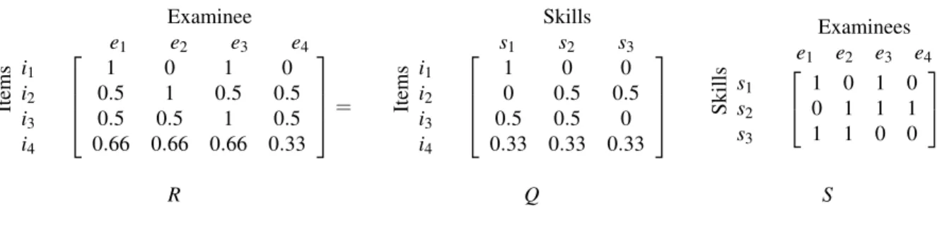
The other type is the additive model of Q-matrix. Compensatory or additive model of skills is an interpre-tation of a Q-matrix where skills have weights to yield a success for that item. For example, considering an item that requires two skills a and b with the same weight each. Then each skill will contribute equally to yield a success of the item. In the compensatory model of Q-matrix, each skill increases the chance of success based on its weight. It is possible to have different weights for skills where skills for each item will sum up to 1. Figure 2.6 represents an example of an additive model of Q-matrix with its cor-responding result matrix. The value Ri j can be considered as a probability that examinee i can succeed
item j. Examinee e1 e2 e3 e4 Items i1 i2 i3 i4 1 0 1 0 0.5 1 0.5 0.5 0.5 0.5 1 0.5 0.66 0.66 0.66 0.33 = Skills s1 s2 s3 Items i1 i2 i3 i4 1 0 0 0 0.5 0.5 0.5 0.5 0 0.33 0.33 0.33 Examinees e1 e2 e3 e4 Skills s1 s2 s3 1 0 1 0 0 1 1 1 1 1 0 0 R Q S
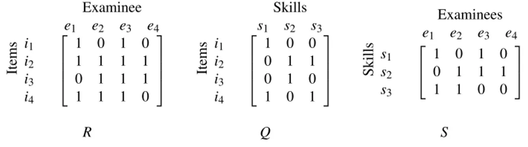
Finally, for the disjunctive model of a Q-matrix, at least one of the required skills should be mastered in order to succeed that item. Figure 2.7 shows an example of this type. For example examinee e3has both
skills S1and S2and all items require either S1or S2; then he should be able to answer all items in the test
outcome. Examinee e1 e2 e3 e4 Items i1 i2 i3 i4 1 0 1 0 1 1 1 1 0 1 1 1 1 1 1 0 Skills s1 s2 s3 Items i1 i2 i3 i4 1 0 0 0 1 1 0 1 0 1 0 1 Examinees e1 e2 e3 e4 Skills s1 s2 s3 1 0 1 0 0 1 1 1 1 1 0 0 R Q S
Figure 2.7 An example for Disjunctive model of Q-matrix
Comparing these three types together, given the same condition for student skills mastery level, one can find out that the average success rate in the test result data is the highest for disjunctive type and the lowest for conjunctive type.
2.5.2 Non-Negative Matrix Factorization (NMF)
Different techniques and methods in the field of data mining were used to derive a Q-matrix. Matrix factorization is one of the most important one in this area. Matrix factorization is a method to decompose a matrix into two or more matrices. Singular Value Decomposition (SVD) and NMF are well known examples of such methods. Beyond skill modeling, it is an important technique in different fields such as bioinformatics, and vision, to name but a few. It has achieved great results in each of these fields. For skills assessment, using tensor factorization, a generalization of matrix factorization to a hypercube instead of matrix and where one dimension represents the time, Thai-Nghe et al. (Thai-Nghe et al., 2011) have shown that the approach can lead to assessments that reach prediction accuracies comparable and even better than well established techniques such as Bayesian Knowledge Tracing (Corbett and Anderson, 1995). Matrix factorization can also lead to better means for mapping which skills can explain the success to specific items. In this research, we use NMF as a skill assessment method that infers a Q-matrix with multiple skills.
Assume R is a result matrix containing student test results of n items (questions or tests) and m stu-dents. NMF decompose the non-negative R, as the product of two non-negative matrices as shown in equation(2.2):
R ≈ QS (2.2)
where Q and S are n × k and k × m respectively. Q represents a Q-matrix which maps items to skills and S represents the skill mastery matrix that represents the mastered skills for each student. k is called as the rank of factorization which is the same as number of latent skills. Equation 2.2 represents an additive
type of Q-matrix.
For example in the following equation, assume that we know the skills behind each item which means we know the exact Q-matrix and also we know the skills mastery matrix as well. In this example the product of Q and S will reproduces the result matrix. Given a result matrix, we want to decompose this result matrix into the expected Q-matrix and skill mastery matrices. Since the Q-matrix is a single skill per item, the type of Q-matrix does not affect the inference of the result matrix.
Examinee Items 1 0 1 0 1 1 0 0 1 0 1 0 0 1 0 1 = Skills Items 1 0 0 0 0 1 1 0 0 0 1 0 × Examinees Skills 1 0 1 0 0 1 0 1 1 1 0 0 R Q S
The prominent characteristic of NMF is the non-negative constraint on the decomposed elements. NMF imposes this constraint and consequently all those values in the decomposed elements are non-negative. The clear point of this decomposition is that there can be different solutions. Although the constraint of non-negative elements eliminates some solutions, there remain many different solutions for this factor-ization.
Considering the large space of solutions to R ≈ QS, different algorithms may lead to different solutions. Many algorithms for matrix factorization search the space of solutions to equation (2.2) by gradient descent. These algorithms can be interpreted as rescaled gradient descent, where the rescaling factor is optimally chosen to ensure convergence. Most of factorization algorithms operate iteratively in order to find the optimal factors. At each iteration of these algorithms, the new value of Q or S (for NMF) is found by multiplying the current value by some factor that depends on the quality of the approximation in Eq. (2.2). It was proved that repeated iteration of the update rules is guaranteed to converge to a locally optimal factorization (Seung and Lee, 2001). We refer the reader to (Berry et al., 2007) for a more thorough and recent review of this technique which has gained strong adoption in many different fields.
Gradient decent is one of the best known approaches for implementing NMF. If k is less than the mini-mum of m and n, finding the exact Q and S matrices which satisfy R = QS, can entail a loss of informa-tion. Therefore this algorithm tries to get the best estimation for Q and S to make R ≈ QS more accurate. Based on the definition of gradient descent method, a cost function should be defined to quantify the quality of the approximation. This cost function can be a measure of distance between two non-negative matrices R and QS. It can be the Euclidean distance between these two matrices as shown in equation (2.3) where Qiis a row vector of Q and Sjis a column vector of S and Ri j is cell (i, j) of R.
kR − QSk2=
∑
i j(Ri j− QiSj)2 (2.3)
Another cost function is based on the Kullback-Leibler divergence, which measures the divergence be-tween R and QS as shown in equation (2.4).
D(R||QS) =
∑
i j (Ri jlog Ri j QiSj − Ri j+ QiSj) (2.4)In both approaches, the goal is to minimize the cost function where they are lower-bounded by zero and it happens only if R = QS (Seung and Lee, 2001). For simplicity we just consider the cost function based on the Euclidean distance.
The gradient descent algorithm used to minimize the error is iterative and in each iteration we expect a new estimation of the factorization. We will refer to the estimated Q-matrix as ˆQ and the estimated Skill mastery matrix as ˆS. The iterative gradient descent algorithm should change Q and S to minimize the cost function. This change should be done by an update rule. Seung and Lee (2001) found the following update rule in equation (2.5). These update rules in equation (2.5) guarantee that the Euclidean distance kR − QSk is non increasing during the iteration of the algorithm.
ˆS ← ˆS ( ˆQTR)
( ˆQTQ ˆS)ˆ Q ← ˆˆ Q
(R ˆST)
( ˆQ ˆS ˆST) (2.5)
The initial value for Q and S are usually random but they can be adjusted to a specific method of NMF library to find the best seeding point.
Barnes (2005) proposed equation 2.6 for conjunctive model of Q-matrix where the operator ¬ is the boolean negation that maps 0 values to 1 and other values to 0. This way, an examinee that mastered all required skills for an item will get 1 in the result matrix otherwise he will get a 0 value, even if the required skills are partially mastered.
In fact if we apply a boolean negation function to both sides of the equation 2.6, we will see that the ¬R matrix is a product of two matrices, Q and ¬S
R = ¬ (Q (¬S)) (2.6)
Later in this chapter the application of NMF on conjunctive type of Q-matrix and how this technique can derive a Q-matrix from a test result is given in details.
Besides its use for student skills assessment and for deriving a Q-matrix, matrix factorization is also a widely used technique in recommender systems. See for eg. Koren et al. (2009) for a brief description of some of the adaptation of these techniques in recommender systems.
2.5.3 Deterministic Input Noisy And/Or (DINA/DINO)
The other skills assessment models we consider are based on what is referred to as Deterministic Input Noisy And/Or (DINO/DINA) Junker and Sijtsma (2001). They also rely on a Q-matrix and they can not in themselves infer a Q-matrix from a test result matrix, and instead require a predefined Q-matrix for the predictive analysis. The DINA model (Deterministic Input Noisy And) corresponds to the conjunctive model whereas the DINO (Deterministic Input Noisy Or) corresponds to the disjunctive one, where the mastery of a single skill is sufficient to succeed an item. The acronyms makes reference to the AND/OR gates terminology.
These models predict item outcome based on three parameters: the slip and guess factors of items, and the different “gate” function between the student’s ability and the required skills. The gate functions are equivalent to the conjunctive and disjunctive vector product logic described for the matrix factorization above. In the DINA case, if all required skills are mastered, the result is 1, and 0 otherwise. Slip and guess parameters are values that generally vary on a [0, 0.2] scale. In the DINO case, mastery of any skills is sufficient to output 1. Assuming ξ is the output of the corresponding DINA or DINO model and sj
and gj are the slip and guess factors, the probability of a successful outcome to item Xi j is:
P(Xi j= 1 | ξi j) = (1 − sj)ξi jg 1−ξi j
j (2.7)
The DINO model is analog to the DINA model, except that mastery follows the disjunctive framework and therefore ξi j = 1 if any of the skills required by item j are mastered by student i.
A few methods have been developed to estimate the slip and guess parameters from data and we use the one implemented in the R CDM package (Robitzsch et al., 2012).
2.6 Recent improvements
The previous sections of this chapter introduced skills assessment techniques to obtain the predictive performance given a dataset. Recall that these models are used for the purpose of defining a performance space used for assessing model fit, as briefly described earlier and detailed in chapter 3. Let us add to the description of the models a few recent developments that concern how the Q-matrix is determined. The general perspective of section 2.6.1 is to find a way for deriving the Q-matrix from data, along with a Skills mastery matrix. Section 2.6.1 is inspired by Desmarais (2012) that was published in ITS conference. This article aims to find a method to derive these matrices for different types of Q-matrices. Finding the number of latent skills (i.e. the common dimension between matrices Q and S) is another important task that is described in section 2.6.1 . The text of section 2.6.2 is mainly borrowed form Beheshti et al. (2012)’s work that was published on EDM conference. Finally, in section 2.6.3 few methods are introduced to validate tasks to skills mapping which is also applicable for the refinement of a Q-matrix. Parts of section 2.6.3 is taken from Desmarais et al. (2014) publication in EDM conference.
2.6.1 NMF on single skill and multi-skill conjunctive Q-matrix
A few studies have shown that a mapping of skills to items can be derived from data (Winters, 2006; Desmarais, 2011). Winters (2006) showed that different data mining techniques can extract item topics, one of which is matrix factorization. He showed that NMF works very well for synthetic data, but the technique’s performance with real data was degraded. These studies show that only highly distinct topics such as mathematics and French can NMF yield a perfect mapping for real data.
Desmarais (2012) proposed an approach to successfully deriving a conjunctive Q-matrix from simulated data with NMF. The methodology of this research relies on simulated data. They created a synthetic data with respect to conjunctive model of Q-matrix. They proposed a methodology to assess the NMF per-formance to infer a Q-matrix from the simulated test data. This methodology is conducted by comparing the predefined Q-matrix, Q, which was used to generate simulated data with the Q-matrix, ˆQ, obtained in the NMF of equation 2.6.
As expected, the accuracy of recovered Q-matrix degrades with the amount of slips and guesses which are somehow noise factor in their study. They showed that if the conjunctive Q-matrix contains one or two items per skill and the noise in the data remains below slip and guess factors of 0.2, the approach successfully derives the Q-matrix with very few mismatches of items to skills. However, once the data has slip and guess factors of 0.3 and 0.2, then the performance starts to degrade rapidly.
2.6.2 Finding the number of latent skills
A major issue with Q-matrices is determining in advance what is the correct number of skills. This issue is present for both expert defined Q-matrices and for data derived ones as well.
In an effort towards the goal of finding the skills behind a set of items, we investigated two techniques to determine the number of dominant latent skills (Beheshti et al., 2012). The SVD is a known technique to find latent factors. The singular values represent direct evidence of the strength of latent factors. Application of SVD to finding the number of latent skills is explored. We introduced a second technique based on a wrapper approach. In statistical learning, the wrapper approach refers to a general method for selecting the most effective set of variables by measuring the predictive performance of a model with each variables set (see Guyon and Elisseeff (2003)). In our context, we assess the predictive performance of linear models embedding different number of latent skills. The model that yields the best predictive performance is deemed to reflect the optimal number of skills.
The results of this experiment show that both techniques are effective in identifying the number of latent factors (skills) over synthetic data. An investigation with real data from the fraction algebra domain is also reported. Both the SVD and wrapper methods yield results that have no simple interpretation on the real data.
2.6.3 The refinement of a Q-matrix
Very often, experts define the Q-matrix because they have a clear idea of what skills are relevant and of how they should be taught.
Validating of the expert defined Q-matrix has been the focus of recent developments in the field of ed-ucational data mining in recent years (De La Torre, 2008; Chiu, 2013; Barnes, 2010; Loye et al., 2011; Desmarais and Naceur, 2013). Desmarais et al. (2014) compared three data-driven techniques for the validation of skills-to-tasks mappings. All methods start from a given expert defined Q-matrix, and use optimization techniques to suggest a refined version of the skills-to-task mapping. Two techniques for this purpose rely on the DINA and DINO models, whereas one relies on a matrix factorization technique called ALS (see (Desmarais and Naceur, 2013) for more details on ALS technique).
To validate and compare the effectiveness of each technique for refining a given Q-matrix, they follow a methodology based on recovering the Q-matrix from a number perturbations: the binary value of a num-ber of cells of the Q-matrix is inverted, and this “corrupted” matrix is given as input to each technique. If the technique recovers the original value of each altered cell, then we consider that it successfully “re-fined” the Q-matrix. The results of this experiment show that all techniques could recover alterations but the ALS matrix factorization technique shows a greater ability to recover alterations than the other two techniques.
2.7 Model selection and goodness of fit
In educational data mining, or in data mining in general, analysts who wish to build a classification or a regression model over new and unknown data are faced with a very wide span of choices. Model selection in EDM is the task of selecting a statistical student model for a given data from a set of candidate models that are the best representatives of the data. Note that there could be a pre-processing step on the data itself to be well-suited to the problem of model selection but our study goes beyond that. The best fit is the model that is most likely to have generated the data. Selection is most often based on a model’s “goodness of fit”. The simplest way is to choose the best performer model. Models with higher predictive accuracy yield more useful predictions and are more likely to provide an accurate description of the ground truth. On one hand the term “goodness of fit” for a statistical model describes how well it fits a set of observa-tion. The distance between observed values and the predicted values under the model can be a measure of goodness of fit. The goodness of fit is usually determined using different measures, namely the best known is likelihood ratio. There exist different approaches to assess model fit based on the measure of goodness of fit. Below we describe few measures that are commonly used:
2.7.1 Measures for goodness of fit
To find the prediction quality of each skills assessment model some metrics are used. There is a wide range of choices of metrics to evaluate a model and choosing an appropriate one is very important since usually candidate models are preforming with small differences and a good metric can highlight the
benefits of one model vs. others.
There are different measures to represent the goodness of fit and this is usually either the sums of squared error (SSE) or maximum likelihood. Dhanani et al. (2014) in a survey compared three error metrics for learning model parameters in Bayesian Knowledge Tracing(BKT) framework (Corbett and Anderson, 1994). In their methodology they calculate the correlation between the error metrics to predict the BKT model parameters and the euclidean distance to the ground truth. These error metrics have been widely used in model selection researches. Below we will describe these metrics briefly:
— The maximum likelihood function selects a set of values for the model parameters that maxi-mizes the likelihood function which also maximaxi-mizes the agreement of the selected model with the observed data. Likelihood function is also called inverse probability, which is a function of the parameters of a statistical model given an observed outcome. This allows us to fit many different types of model parameters. This measure is mostly for estimating parameters and in next sections of this chapter we will see its application in model selection. Since in our study the student test result follows a binomial distribution then the likelihood can be defined as equation 2.8.
Likelihood(data) = n
∏
i=1 pyi i (1 − pi)(1−yi) (2.8)where pi and yiare the estimated and actual values of ith datapoint. Applying natural logarithm
on the right side of equation 2.8 will results log-likelihood. Hence it becomes more convenient in maximum likelihood estimation because logarithm is a monotonically increasing function. — Sum of squared errors of predictions (SSE) is the other measure which is the total deviation of the
response values from the predicted values as represented in equation 2.9
SSE(data) =
n
∑
i=1(yi− pi)2 (2.9)
A more informative measure is RMSE which the squared root of the mean squared errors:
RMSE(data) = s 1 n n
∑
i=1 (yi− pi)2 (2.10)— There is another category of metrics that is widely used for classification purposes and we also use in our experiments to compare the ground truth prediction of two model selection approaches for a given data. These metrics rely on the confusion table, which allows us to calculate the accuracy, recall, precision and F-measure values. A confusion matrix is a table that shows the performance of a classification method. A model selection method can also be tested as a classification method to classify the ground truth as we will show later in section 3.2.4. Below a confusion table is presented where each row represents the number of instances in the actual class and each column represents the instances in the predicted class: