Design of robust networks.
Application to the design of wind farm cabling networks.
THOMAS RIDREMONT
Département de mathématiques et de génie industriel Polytechnique Montréal
et
Conservatoire National des Arts et Métiers
Thèse en cotutelle présentée en vue de l’obtention du diplôme de Philosophiæ Doctor Mathématiques
Avril 2019
c
Cette thèse intitulée :
Design of robust networks.
Application to the design of wind farm cabling networks.
présentée par Thomas RIDREMONT
en vue de l’obtention du diplôme de Philosophiæ Doctor a été dûment acceptée par le jury d’examen constitué de :
Sourour ELLOUMI, présidente
Alain HERTZ, membre et directeur de recherche
Marie-Christine COSTA, membre et codirectrice de recherche Cédric BENTZ, membre et codirecteur de recherche
Miguel ANJOS, membre Frédéric ROUPIN, membre Dritan NACE, membre
ACKNOWLEDGEMENTS
First of all, I would like to thank my thesis directors: Marie-Christine Costa, Cédric Bentz and Alain Hertz. Thank you for sharing with me your passion for operations research. Thank you for being present, patient, available, for accompanying me in my research project, with good humour, enthusiasm and kindness. Thank you to Marie-Christine and Cédric for being particularly present and responding at the end of a thesis where I particularly solicited them. Thank you to Alain for welcoming me perfectly to Montreal, for being very available, even when an ocean separated us.
Thanks to Dominique Quadri and Miguel Anjos, who did me the honour of being the rap-porteurs of my thesis. Thank you for your time, interest and comments. Thank you also to Sourour Elloumi, Dritan Nace and Frédéric Roupin for the honour of serving on my thesis jury.
Thank you to the people of CEDRIC for their advice, their good humour, their help but above all the good working atmosphere, as well as to the members of GERAD and UMA. I am thinking of Amélie, Agnès, Alain B., Alain F., Christophe, Daniel, Éric, Maurice, Safia, Sami, Sourour, Stéphane and Zacharie, among others. Thank you to all those with whom I was able to share my office, I think in particular of Pierre-Louis and Dimitri, who welcomed me and with whom I learned a lot, thank you to Arnaud, whom I welcomed, and to Antoine and Hadrien.
Thank you to my friends in Montreal, who made me feel at home there. Thanks to my friends from Angers and Paris too, who have been present during these few years, thanks to Brice and Sylvain for welcoming me with open arms at several times. A special thank you to my friend Florian, who was very supportive throughout my thesis and with whom I was able to discuss the life of a doctoral student. Thank you to Camille, who supported me in the last moments of the thesis, thanks for her patience, tenacity, attention and especially her understanding.
Finally, a big thank you to my family, my grandparents and my grandmother. Thank you to them who have been able to support me throughout this period, to help me when I needed it, especially at the end of this thesis. Thanks to Anaëlle and Clara, for their good humour. Thank you to my brother Damien, with whom I shared a lot and who always listened to me. Thank you to my father, who was able to give me his advice, and thank you to my mother, who is always a great help and who gave me a lot of time.
RÉSUMÉ
Aujourd’hui, la conception de réseaux est une problématique cruciale qui se pose dans beau-coup de domaines tels que le transport ou l’énergie. En particulier, il est devenu nécessaire d’optimiser la façon dont sont conçus les réseaux permettant de produire de l’énergie. On se concentre ici sur la production électrique produite à travers des parcs éoliens. Cette énergie apparait plus que jamais comme une bonne alternative à la production d’électricité via des centrales thermiques ou nucléaires.
Nous nous intéressons dans cette thèse à la conception du câblage collectant l’énergie dans les parcs éoliens. On connaît alors la position de l’ensemble des éoliennes appartenant au parc ainsi que celle du site central collecteur vers laquelle l’énergie doit être acheminée. On con-naît également la position des câbles que l’on peut construire, leurs capacités, et la position des nœuds d’interconnexion possibles. Il s’agit de déterminer un câblage de coût minimal permettant de relier l’ensemble des éoliennes à la sous-station, tel que celui-ci soit résistant à un certain nombre de pannes sur le réseau.
Mots clés: Recherche opérationnelle, Optimisation combinatoire, Conception de réseaux ro-bustes, Théorie des graphes, Programmation en nombres entiers, Câblage de parcs éoliens.
ABSTRACT
Nowadays, the design of networks has become a decisive problematic which appears in many fields such as transport or energy. In particular, it has become necessary and important to optimize the way in which networks used to produce, collect or transport energy are designed. We focus in this thesis on electricity produced through wind farms. The production of energy by wind turbines appears more than ever like a good alternative to the electrical production of thermal or nuclear power plants, giving that both of those production can have harmful consequences on the environment. It has then become necessary to optimize the design and construction of such networks.
We focus in this thesis on the design of the cabling network which allows to collect and route the energy from the wind turbines to a sub-station, linking the wind farm to the electrical network. In this problem, we know the location of each wind turbine of the farm and the one of the sub-station. We also know the location of possible inter-connection nodes which allow to connect different cables between them. Each wind turbine produces a known quantity of energy and with each cable are associated a cost and a capacity (the maximum amount of energy that can be routed through this cable). The optimization problem that we consider is to select a set of cables of minimum cost such that the energy produced from the wind turbines can be routed to the sub-station in the network induced by this set of cables, without exceeding the capacity of each cable. We focus on cabling networks resilient to breakdowns.
Keywords : Operations Research, Combinatorial optimization, Robust networks design, Graph theory, Mixed integer programming, Wind farm cabling networks.
TABLE OF CONTENTS ACKNOWLEDGEMENTS . . . iii RÉSUMÉ . . . iv ABSTRACT . . . v TABLE OF CONTENTS . . . vi LIST OF TABLES . . . ix LIST OF FIGURES . . . x CHAPTER 1 INTRODUCTION . . . 1 1.1 General introduction . . . 1 1.2 Preliminaries . . . 4
1.2.1 General notions in graph theory . . . 4
1.2.2 Flows and networks . . . 5
1.2.3 Steiner trees and networks . . . 9
1.3 Previous work . . . 10
1.3.1 Wind farm cable layout optimization . . . 10
1.3.2 Steiner arborescence problems . . . 11
1.3.3 Robust Steiner networks . . . 12
1.3.4 The k most vital arcs in flow networks and network interdiction problems 14 CHAPTER 2 ROBUST ARBORESCENCES . . . 16
2.1 Introduction . . . 16
2.2 Definition of problems and complexity results . . . 16
2.3 Mathematical formulations and tests . . . 20
CHAPTER 3 CAPACITATED ROOTED k-EDGE CONNECTED STEINER NET-WORK PROBLEM (CRkECSN) . . . . 31
3.1 Definitions and notations . . . 31
3.2 Formulations . . . 32
3.2.1 Cutset formulation . . . 32
3.2.3 Bilevel formulation . . . 37
3.3 Relations between the formulations . . . 44
3.3.1 Relations between the bilevel and the cutset formulations . . . 44
3.3.2 Relations between the flow and the cutset formulations . . . 48
3.4 Addition of protected arcs . . . 49
3.4.1 Cut-set formulation . . . 50
3.4.2 Equivalence between cut-set and bilevel formulations in the protected case . . . 52
3.4.3 Flow formulation . . . 53
3.5 Valid and strengthening inequalities . . . 53
3.5.1 Case without the possibility of protecting arcs . . . 54
3.5.2 Case with the possibility of protecting arcs . . . 55
3.6 Results analysis . . . 56
CHAPTER 4 A TABU SEARCH FOR THE DESIGN OF CAPACITATED ROOTED k-EDGE CONNECTED STEINER PLANAR NETWORKS . . . . 68
4.1 Introduction . . . 68
4.2 Testing survivability . . . 68
4.3 Tabu Search . . . 73
4.3.1 A repair procedure . . . 75
4.3.2 Inclusion-wise minimal solutions . . . 77
4.3.3 The proposed tabu search for the CRkECSN . . . 79
4.4 Computational Experiments . . . 81
CHAPTER 5 WIND FARM CABLE LAYOUT OPTIMIZATION WITH CONSTRAINTS OF LOAD FLOW AND ROBUSTNESS . . . 89
5.1 Introduction . . . 89
5.1.1 Presentation of the problem . . . 89
5.1.2 The Load Flow constraints . . . 90
5.2 The problem without breakdowns . . . 94
5.2.1 Mathematical formulation . . . 94
5.2.2 Variables and constraints . . . 95
5.2.3 Mathematical program . . . 97
5.2.4 Linearization of the program . . . 98
5.3 Robust approach . . . 99
5.3.1 The case k = 1 . . . . 99
5.4 Results analysis . . . 105 CONCLUSION AND RECOMMENDATIONS . . . 107
LIST OF TABLES
Table 2.1: Results on robust arborescences and data parameters . . . 26
Table 3.1: Instance parameters . . . 56
Table 3.2: Results for non-uniform capacities, k = 1 and k0 = 0 . . . 58
Table 3.3: Results for non-uniform capacities, k = 2 and k0 = 0 . . . 59
Table 3.4: Results for non-uniform capacities, k = 3 and k0 = 0 . . . 60
Table 3.5: Results for non-uniform capacities, k = 1 and k0 ∈ {1, 2, 3} . . . . . 61
Table 3.6: Results for non-uniform capacities, k = 2 and k0 ∈ {1, 2, 3} . . . . . 61
Table 3.7: Results for non-uniform capacities, k = 3 and k0 ∈ {1, 2, 3} . . . . . 63
Table 3.8: Results for uniform capacities and k = 1 . . . . 64
Table 3.9: Results for uniform capacities and k = 2 . . . . 65
Table 3.10: Results for uniform capacities and k = 3 . . . . 66
Table 4.1: Results for k = 1 where (i, j) ∈ A if and only if (j, i) ∈ A. . . . 85
Table 4.2: Results for k = 2 where (i, j) ∈ A if and only if (j, i) ∈ A. . . . 86
Table 4.3: Results for k = 3 where (i, j) ∈ A if and only if (j, i) ∈ A. . . . 86
Table 4.4: Results for k = 1 where (i, j) /∈ A if (j, i) ∈ A. . . . 87
Table 4.5: Results for k = 2 where (i, j) /∈ A if (j, i) ∈ A. . . . 88
Table 4.6: Results for k = 3 where (i, j) /∈ A if (j, i) ∈ A. . . . 88
Table 5.1: Results of the tests for the non-robust case and for the robust case with k = 1 . . . . 106
LIST OF FIGURES
Figure 1.1: Example of graph transformation for the vertex v . . . . 9
Figure 2.1: Graph and RSpAF solution resulting from the 3-Partition instance in which m = 2, B = 11, D = {5, 3, 4, 3, 4, 3} . . . . 20
Figure 2.2: Resulting arborescence for the fourth data set for CStA . . . . 27
Figure 2.3: Resulting arborescence for the fourth data set for RCStA . . . . 28
Figure 2.4: Resulting arborescence for the fourth data set for BRCStA . . . . . 29
Figure 2.5: Resulting arborescence for the fourth data set for BRCStAbounded−robust−cost 30 Figure 3.1: Example of addition of a sink to the input graph . . . 33
Figure 3.2: Graph where Inequalities (3.24a) and (3.24b) cut some non-integer solutions . . . 54
Figure 3.3: Cost of the solutions for different instances . . . 67
Figure 4.1: Construction ofGf0 from G0 . . . 69
Figure 4.2: justification=centering . . . 70
Figure 4.3: Construction of 2D e G0 for the graph Gf0 of Figure 4.1 . . . 72
CHAPTER 1 INTRODUCTION
1.1 General introduction
In the 21st century, it appears that the biggest challenge that will face our population is the
global warming. The air temperature has been increased by 1.5 degrees since preindustrial era and this rise has been linked to human activities. Almost all specialists among the com-munity agree that the major cause of this global warming can be attributed to the increasing production of greenhouse gas (caused by carbon monoxide emission or methane principally). The consequences could be diverse and terrible: for the climate (for example extreme heat in some parts of the globe or increase of extreme weather events like storms, floods, cyclones and droughts); for the ecosystem and the biodiversity (increase of ocean levels, destruction of fragile ecosystems like coral reef and Amazon rainforest and several extinctions of species); on our society and its economy (infrastructures to adapt like medical ones or housings, public health and capacity to feed the population). Many forces appear to fight the global warm-ing and involve ecology in our way of life (reducwarm-ing our consumption of energy, limitwarm-ing the food waste, optimizing the management of resources, avoiding to consume products with a high carbon print). Sustainable development, which aims to exploit natural and biological resources at a rhythm which does not lead impoverishment or even exhaustion but makes possible the sustain of biological productivity of resources in the biosphere, comes out as a valid orientation in order to limit those consequences. Regarding the electrical production, wind farms, photo-voltaic panels and hydro-electrical facilities appear to be interesting di-rections in order to reduce greenhouse gas emissions.
Nowadays, the design of networks has become a decisive problematic which appears in many fields such as transport, telecommunications or energy. In particular, it has become impor-tant and even necessary to optimize the way in which networks used to produce, collect or transport energy are designed. We are interested in this thesis on electricity produced through wind farms. The production of energy by wind turbines appears more than ever like a good alternative to the electrical production of thermal or nuclear power plants, giving that both of those productions can have harmful consequences on the environment. The develop-ment of wind farms is then a global issue and hence it has become necessary to optimize the design and construction of such networks.
the energy from the wind turbines to a sub-station, linking the wind farm to the electrical network. In this problem, we know the location of each wind turbine of the farm and the one of the sub-station. We also know the location of possible inter-connection nodes which allow to connect different cables between them. Each wind turbine produces a known quantity of energy and with each cable are associated a cost and a capacity (the maximum amount of energy that can be routed through this cable). The optimization problem that we consider is to select a set of cables of minimum cost such that the energy produced from the wind turbines can be routed to the sub-station in the network induced by this set of cables, without exceeding the capacity of each cable. Hence there must exist a path using cables between each turbine and the substation, but not necessarily with inter-connection nodes, which are optional points in the network.
In this context, breakdowns can occur on cables or devices of the network (caused by the environment or by a problem with a turbine or inter-connexion node for example). We focus more precisely on the design of robust (or resilient) networks for several robust notions that will be defined in this thesis. We take into account some data incertitude: we consider the case of breakdowns on cables or nodes once the network is built (in this thesis we focus on breakdowns on cables, but breakdowns on nodes can be reduced to breakdowns on cables after a transformation of the graph). We then aim to minimize the cost of the network to build while respecting robustness constraints allowing to limit the damaging repercussions in case of a breakdown on one or several cables in the network.
In the context of this thesis, we have been in contact with EDF (Électricité de France), first producer and supplier of electricity in France, via PGMO (Programme Gaspard Monge pour l’Optimisation de la Fondation Mathématique Jacques Hadamard) and engineers working in the field of renewable energy networks. It appears that combinatorial and discrete aspects of those problems have been sparsely studied until now at EDF. Although the design of the cabling networks presents high economic stakes, robustness and resilience to breakdowns are important criteria too. Some work has also been done with the Canadian company Hatch, which led us to test our work on real data (we can underline that the French wind farms we have been working on with EDF are offshore whereas Canadian wind farms are onshore). In offshore environment, each wind turbine produces about the same quantity of electricity, so we can make the assumption that the energy produced by the wind turbines is uniform.
farm cabling networks by reformulating the set of electricity constraints into classical flow constraints (like Chapters 2, 3 and 4) and practical problems with real data and technical constraints related to electricity (Chapter 5). We study problems which are generalizations of the Steiner tree problem: given a graph with a set of vertices, a set of edges and a subset of vertices called terminals, this problem aims at finding a tree of minimum cost spanning all the terminals. The vertices which are not terminals are called Steiner vertices. We introduce a root vertex in our problems. In our wind-farm application, the wind turbines correspond to the terminals, the substation to the root, and the inter-connection nodes to the Steiner vertices. We aim at solving generalizations of Steiner tree problems taking robustness and edge capacities into account.
In Chapter 1.2, we introduce and define some notions, notations and methods used in this thesis. We also define the studied problematics. We present some preliminary results and summarize some previous works found in the literature.
Following discussions with EDF engineers, it appeared that the electrical constraints can be formulated as classical flow constraints if the solution network is an arborescence. Hence, in Chapter 2, we reduce the problem to the search for a Steiner arborescence which respects the capacity constraints. We focus on the design of Steiner arborescences for which we try to reduce the damaging impact of an arc deletion in the arborescence solution, according to several optimization criteria, at a reasonable cost. We give complexity results and propose several formulations tested on real data.
In our wind farm applications, the terminals produce energy, so the energy flow should be routed from the terminals to the root. However, it is equivalent to consider that we route the energy from the root to the terminals (in a digraph, we just have to take the opposite arcs whereas there are no changes in an undirected graph). Furthermore, in offshore wind farm applications, we often consider that the energy produced by the wind turbines is uniform, which is equivalent to consider a unit demand and an arc capacity can then be seen as the number of terminals that can be linked to the root through this arc.
In Chapter 3, we define the Capacitated Rooted k-Edge Connected Steiner Network: given a connected graph with a root vertex, a set of terminals and integer capacity and cost on each arc of the graph, we aim to find a subset of arcs of minimum cost such that there exists a feasible flow (i.e. respecting the capacities) routing one unit of flow from the root
to each terminal in the subgraph induced by those arcs, even if a given number k of arcs is deleted. This problem is equivalent to finding a robust cabling network in a wind farm, when the electricity constraints are formulated as classical flow constraints. We give several formulations, including a new bilevel formulation, study the relations between the different formulations, and test them in order to compare their efficiency.
In Chapter 4, we focus on planar graphs for the Capacitated Rooted k-Edge Connected Steiner Network. We present a method to check whether a network is resilient or not to the deletion of any set of k arcs using planar graph duality and shortest paths problems. We propose and describe a tabu search algorithm derived from this method. We test our algorithm and compare its efficiency to exact methods presented in Chapter 3.
In Chapter 5, we study the real-life problem of designing a wind farm cabling network with electrical constraints of load flow. We explain the load flow study, which corresponds to a numerical analysis of the flow of electric power in an interconnected system. We must ensure that the power routed through each cable respects the electric capacities of the cable using the load flow equations to analyze the state of the electric network once the network is built. Since the load flow analysis is a non-linear system, we use an approximation in order to include them into a mixed-integer linear program. We test our algorithm on real data and give numerical results.
In a concluding chapter, we give some perspectives and future work leads.
1.2 Preliminaries
1.2.1 General notions in graph theory
In this section, we recall some notions from graph theory that will be used in this thesis. For more information about graph theory, the reader is referred to [12, 63].
Formally, a directed graph (or digraph) G = (V, A) is defined by a set of vertices V and a set of arcs A ⊆ V × V . The set of predecessors (respectively successors) of a vertex v in G is defined by Γ−G(v) (respectively Γ+G(v)). For a subset of vertices S ⊂ V in G, we define δG−(S) = {(i, j) ∈ A | i ∈ V \ S, j ∈ S} (respectively δG+(S) = {(i, j) ∈ A | i ∈ S, j ∈ V \ S}) as the set of arcs entering (resp. leaving) S. When there are no ambiguities about the related graph G, we can refer to those sets as Γ−(v), Γ+(v), δ−(S) and δ+(S), respectively.
An undirected graph G0 = (V, E) is defined by a set of vertices V and a set of edges E ⊆ V ×V . The set of neighbors of a vertex v ∈ V is denoted by ΓG0(v). For a subset of vertices S ⊂ V in G0, we define δG0(S) as the set of edges [u, v] incident to S in G0 (u ∈ S and v ∈ V \ S). When there are no ambiguities about the related graph G0, we can refer to those sets as Γ(v) and δ(S) respectively.
Two paths p1 and p2 in a graph are said to be arc-disjoint (edge-disjoint in an undirected
graph) if there is no arc a which appears both in p1 and p2. In this thesis, we will consider a
special vertex r of a graph G, which is the root of the graph (i.e. there exists a path between r and every vertex of G). A graph is said to be connected if there is an undirected path between u and v for each pair of vertices u, v ∈ V2. In a digraph G = (V, A) (resp. an
undirected graph G = (V, E)), an (i, j)−disconnecting set, with i and j two distinct vertices of V , is a set of arcs D ⊆ A (resp. a set of edges D ⊆ E) such that there are no path from i to j in the graph G0 = (V, A \ D) (resp. G0 = (V, E \ D)). A graph (respectively digraph) is said to be k-edge-connected (resp. k-arc-connected) if it remains connected (resp. strongly connected) whenever fewer than k edges (resp. arcs) are removed.
Theorem 1.2.1 (k-edge-connectivity [48]) If i and j are two vertices of a digraph (resp. undirected graph), the minimum size of an (i, j)−disconnecting set is equal to the maximum number of pairwise arc-disjoint (resp. edge-disjoint) paths from i to j. Moreover, a graph G is k-edge-connected if and only if there exist k pairwise arc-disjoint paths (resp. edge-disjoint) between each pair of vertices in G.
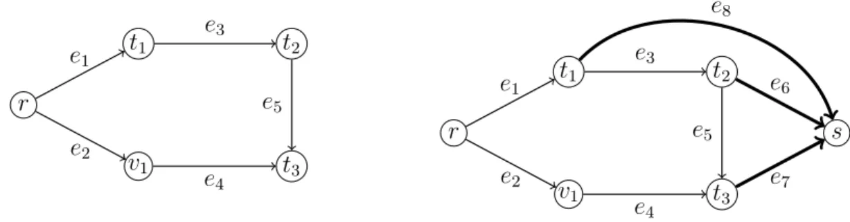
1.2.2 Flows and networks
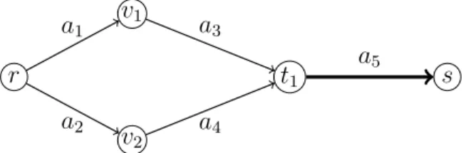
We introduce here different notions about network flows; the reader is referred to [2] for more information about this topic. We define a network as a digraph G = (V, A) with a non-negative capacity uij on each arc (i, j) ∈ A, a distinguished root r ∈ V (also called source
vertex) and a sink vertex s ∈ V . A flow x is a function that assigns a value xij to each arc
(i, j) ∈ A. A feasible flow satisfies the capacity constraints 0 ≤ xij ≤ uij for each arc (i, j) ∈ A
and the conservation constraints P
u∈Γ−(v)xuv =Pw∈Γ+(v)xvw for each vertex v ∈ V \ {r, s}. The value of such a flow is equal to P
v∈Γ+(r)xrv−Pu∈Γ−(r)xur =Pi∈Γ−(s)xis−Pj∈Γ+(s)xsj. In this thesis, we assume without loss of generality that, in any network we consider, there are no arcs entering the root r and no arcs leaving the sink s. Thus, the value of a flow
x is equal to P
v∈Γ+(r)xrv = Pi∈Γ−(s)xis. A maximum flow is defined as a feasible flow of maximum value.
In a network, for a given subset of vertices S ⊂ V with r ∈ S and s ∈ V \ S, we refer to the partition [S, V \ S] of V as an r − s cut. The cut-set associated with S is the set of arcs going from a vertex of S to a vertex of V \ S, i.e. the cut-set corresponds to δ+(S) or δ−(V \ S).
The capacity of a cut (or the capacity of a cut-set) is defined as the sum of the capacities of the arcs of its cut-set, i.e. P
(i,j)∈δ+(S)uij. We recall the well-known following theorem: Theorem 1.2.2 (Max-flow min-cut theorem [29]) In a network with a root r and a sink s, the minimum capacity of a r − s cut is equal to the maximum value of a feasible flow from r to s.
The problem of searching for a maximum flow (respectively a minimum r−s cut) in a network is called the maximum flow problem (respectively the minimum cut problem). The flow xij
on each arc (i, j) ∈ A is not constrained to be integer. However, in this thesis we will work on integer flows because of the applications we are considering. Thus, we remind the following theorem:
Theorem 1.2.3 (Integrality Theorem [2]) If all capacities in a network are integer, then there exists a maximum flow in which the amount of flow on each arc is integer. Furthermore, a maximum flow can be partitioned into flows of integer values along paths from the root to the sink.
Theorem 1.2.3 allows to relax the integrality constraint on the value of the flow when searching for a maximum flow. We introduce the following well-known linear formulation for the maximum flow problem:
(M AX − F LOW ) max x X v∈Γ+(r) xrv s.t. X i∈Γ−(j) xij− X k∈Γ+(j) xjk = 0 ∀j ∈ V \{r, s} 0 ≤ xij ≤ uij ∀(i, j) ∈ A (1.1a) (1.1b)
where the variable xij defines for each arc (i, j) the amount of flow routed through (i, j). We
Remark 1.2.1 If there exist two vertices i and j in V \ {r, s} such that {(i, j), (j, i)} ⊂ A and a flow defined by x such that xij > 0 and xji > 0, then there always exists a flow x0 of
equal value with either x0ij = 0 or x0ji = 0.
Proof: Let us suppose that a given feasible flow x assigned to a network G = (V, A) is such that there exist two vertices i and j in V such that (i, j), (j, i) ∈ A and there is a positive amount of flow on both arcs (i.e. xijxji > 0). By reducing the flow on both arcs
by min(xij, xji), we find a flow x0 with either x0ij = 0 or x0ji = 0. The capacity constraints
are obviously satisfied because we only reduce the amount of flow on two arcs and they were satisfied by x. The conservation constraints are also satisfied since we reduce the amount of flow entering and leaving both i and j by min(xij, xji). Finally, the value of the flow defined
by x remains the same because P
i∈Γ−(s)xis is not changed. 2
A matrix A is said to be totally unimodular if each square submatrix of A has a determinant equal to −1, 0 or 1 (see [58]). In particular, we have that each entry of A is −1, 0 or 1. Theorem 1.2.4 (Theorem 5.20 in [58]) Let A be a totally unimodular m × n matrix and let b ∈ Zm. Then the polyhedron
P = {x|Ax ≤ b} is integer.
We have the following property and theorem on the totally unimodular matrices:
Property 1.2.1 Let A be a totally unimodular m × n matrix and Im the m × m identity
matrix. We have that −A, A> and [A|Im] are totally unimodular matrices.
The matrix M associated with the left-hand side of Constraints (1.1a) is a sub-matrix of the node-arc incidence matrix (we remove the rows associated to r and s) of a digraph. Each column of the matrix corresponds to an arc (i, j): there is a 1 in the ith row and a −1 in the jth row and the rest of the entries of the column are 0.
Theorem 1.2.5 (Theorem 11.12 in [2]) The node-arc incidence matrix M of a directed network is totally unimodular.
Following Theorems 1.2.4 and 1.2.5, we do not have to ensure that x is integer since M is totally unimodular, which yields a proof of Theorem 1.2.3.
The dual of (M AX − F LOW ) corresponds to a formulation of the minimum-cut problem and can be written as follows:
min µ,λ X (i,j)∈A uijλij s.t. µv + λrv ≥ 1 ∀v ∈ Γ+(r) µv − µu+ λuv ≥ 0 ∀(u, v) ∈ A, u 6= r, v 6= s − µu+ λus ≥ 0 ∀u ∈ Γ−(s) λij ≥ 0 ∀(i, j) ∈ A, µv ∈ R ∀v ∈ V \ {r, s} (1.2a) (1.2b) (1.2c)
It can be reformulated, with the addition of variables µr and µs, as follows:
(M IN − CU T ) min µ,λ X (i,j)∈A uijλij s.t. µv− µu+ λuv ≥ 0 ∀(u, v) ∈ A µr = 1 µs = 0 λij ≥ 0 ∀(i, j) ∈ A, µv ∈ R ∀v ∈ V (1.3a) (1.3b) (1.3c)
In any optimal solution we have µv ∈ [0, 1] ∀v ∈ V , which implies λij ≤ 1 ∀(i, j) ∈ A.
From Property 1.2.1, the transpose of a totally unimodular matrix is totally unimodular, so the matrix of constraints of (M IN − CU T ) is totally unimodular, and thus there exists an optimal solution (λ∗, µ∗) with µ∗ ∈ {0, 1}|V | and λ∗ ∈ {0, 1}|A|. The dual problem then
formulates the minimum cut problem in this way: µ defines the partition associated with the cut (we have µv = 1 if v is in the same part as the root and µv = 0 if v is in the same part
as the sink) while λ defines the cut-set (we have λij = 1 if the arc (i, j) is in the cutset, i.e.
µi = 1 and µj = 0).
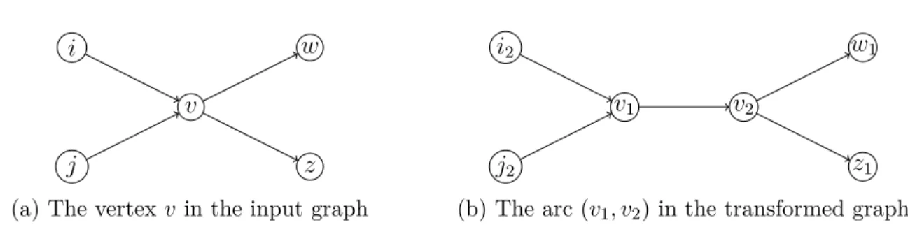
In this thesis, we will consider arc-deletions in flow networks. However, vertices-deletion can be considered using the same methods by a simple transformation of the input graph. The graph transformation is the following: we replace each vertex v of the input graph G by two vertices v1 and v2 and an arc (v1, v2) in the transformed graph and each arc (u, v) is replaced
by an arc (u2, v1). The deletion of the vertex v in the input graph then corresponds to the
deletion of the arc (v1, v2) in the transformed graph (as illustrated in the example in Figure
associated to the input graph. v i j w z
(a) The vertex v in the input graph
v1 v2
i2
j2
w1
z1 (b) The arc (v1, v2) in the transformed graph
Figure 1.1 Example of graph transformation for the vertex v
1.2.3 Steiner trees and networks
We introduce in this subsection the concepts of Steiner trees and Steiner networks (see [25, 40, 52]). A tree is defined as a connected graph which is acyclic. Given an undirected graph G = (V, E) and a subset of vertices T ⊆ V , a subgraph S of G is called a Steiner tree if S is a tree containing all vertices of T . A vertex t ∈ T is called a terminal vertex (or terminal) whereas a vertex v ∈ V \ T is called a Steiner vertex (or Steiner point). The minimum Steiner tree problem can be defined as follows:
Minimum Steiner Tree Problem
INSTANCE: A graph G = (V, E) and a set of terminals T ⊆ V .
PROBLEM: Find a minimum Steiner tree spanning T in G. That is, find a Steiner tree S = (VS, ES) such that |ES| = min{|ES0| | S0 = (VS0, ES0) is a Steiner tree spanning T in G}.
Given a positive cost cefor each edge e ∈ E, we define similarly the Minimum-Cost Steiner
Tree Problem as the problem of finding a Steiner tree S = (VS, ES) for which the sum of
the costs ce0 for e0 ∈ ES is minimum. The Minimum-Cost Steiner Tree problem is N P-hard and generalizes both the Minimum Spanning Tree problem and the Shortest Path problem: if T = V , the Minimum Steiner Tree Problem is equivalent to the Minimum Spanning Tree Problem whereas if |T | = 2, it is equivalent to the Shortest Path problem.
In this thesis, we consider Steiner problems with a root and a capacity uij on each edge [i, j]
in the graph. We consider that each terminal t ∈ T has the same demand and we want to find a feasible flow (i.e. respecting the capacities defined by u and the flow conservation
constraints) such that a unit of flow is routed from the root to each terminal: each terminal can hence be seen as a sink. We say that a feasible flow x routes one unit of flow from the root r to each terminal if the flow conservation constraints are as follows:
X k∈Γ+(j) xjk − X i∈Γ−(j) xij = |T | if j = r −1 if j ∈ T 0 otherwise ∀j ∈ V
If we add to the graph a fictive sink s with an edge (t, s) of capacity uts = 1 for each terminal
t ∈ T , our problem is equivalent to finding a feasible (r − s)-flow of value |T |.
1.3 Previous work
We summarize in this section the existing results in the literature for problems which are related to the ones studied in this thesis.
1.3.1 Wind farm cable layout optimization
The design of wind farms brings several challenges in optimization: one can think of the op-timization of the location of each wind turbine (a literature review for this kind of problems is proposed by Gonzalez et al. [37]) or of the connection between the electric network and the wind farm [53], for example. In this thesis, we will only consider the problem of designing the cabling network that collects the energy produced by the wind turbines and route it to the sub-station, once the locations of the different wind turbines are known.
Problems of designing the wind farm cabling network have already been studied in the litera-ture. Hertz et al. [39] study a real-life problem with real data for onshore wind farms, where several cable types are available (subterranean or not). Furthermore, the energy produced by the wind turbines and routed to the sub-station is non-splittable: once the energy is routed through a same cable, it cannot be split and must be routed to the sub-station through the same path (i.e. if a "chunk" of energy E is routed from u to v through the same cable with v different from the substation, there exists a node w such that the "chunk" E is entirely routed from v to w). The authors give mixed integer formulations and propose a cutting plane generation method allowing to evaluate their algorithm on real data.
Other authors propose mixed integer formulations for the design of wind farm cabling [14, 27]. Regarding offshore wind farms, Pillai et al. [51] propose a set of algorithms computing
ap-proximate solutions in order to optimize successively the location of the wind turbines and the design of the wind farm cabling network considering natural obstacles related to the environment. Fischetti and Pisinger [28] also consider natural obstacles related to the envi-ronment but they additionally consider the power losses related to the routing of electricity. They propose a mixed-integer formulation and a method allowing to find good approximate solutions using matheuristics.
To the best of our knowledge, there does not exist literature proposing a method that could be applied to the problem of designing wind farm cabling networks with resilience to breakdowns on cables and load flow constraints. In this thesis, we are interested in the design of wind farm networks with such constraints.
1.3.2 Steiner arborescence problems
In some cases, production rules and electrical constraints related to the routing of electricity imply that the problem of designing such a wind farm cabling can be seen as the search for a Steiner arborescence with capacity constraints and unitary demands. More precisely, the problem can be defined as follows: we are given a graph with a subset of vertices T and a root r, where each arc has a cost and a capacity. We look for an arborescence rooted at r which contains each vertex of T , and such that, for each arc (i, j) of the arborescence, the number of terminals in the sub-arborescence rooted at j is at most equal to the capacity of (i, j). The problem is then a generalization of the Steiner arborescence problem, but also a particular case of the generalized Steiner arborescence, in which there is a fixed demand at each terminal and each arc capacity corresponds to the quantity of demands which can be routed through this arc.
The minimum-cost (or weighted) Steiner tree problem (without capacity constraints) has been widely studied in the literature; the reader is referred to [25, 40, 52]. It has also many applications in industry; see [22, 26]. This problem is N P-hard even if all edge costs are equal (it corresponds to the Minimum Steiner Tree Problem) and if G is planar [32]. However, if the number of terminals is fixed, this problem can be solved in polynomial time [24].
When taking into account the arc capacities, Papadimitriou shows that the problem is N P-Hard in the spanning case (i.e. all vertices except the root are terminals) [49]. The problem has been studied in the spanning case, and branch-and-bound as well as branch-and-price
algorithms have been proposed [21, 62]. Jothi and Raghavachari [41] and Arkin et al. [4] propose approximation algorithms when capacities are uniform.
Regarding Steiner arborescence problems with capacity constraints, Bentz et al. study the complexity and approximation considering several parameters like the number of terminals, the arc costs and the capacities [10]. Goemans and Myung propose several Steiner tree for-mulations [36]. Bousba et al. solve the Steiner arborescence problem with capacities and demands, which is a generalization of the Steiner tree problem with capacities [20]: each ter-minal has a specific amount of demand that must be routed from the root to this terter-minal, and the capacity of an arc corresponds to the maximum amount of demands that can be routed through this arc.
To the best of our knowledge, the design of Steiner trees with constraints of robustness, i.e. where we aim to design trees which are not too much impacted by arc deletions, has not been studied. However, different problems with arc deletions on trees have been studied. Bazgan et al. [8] study the problem of finding in a graph a subset of k edges whose deletion causes the largest increase in the weight of a minimum spanning tree: they propose an enumeration algorithm and a MIP to solve the problem. This problem has been shown to be N P-hard, and approximation algorithms have been proposed [30, 45]. However, this problem considers the arc deletions before the design of the tree, whereas we consider the arc deletions during the design of the tree.
1.3.3 Robust Steiner networks
Robust problems have been widely studied in continuous optimization [9, 15, 43] and can be seen as problems modeling uncertainty, where the description of uncertainty is a deterministic variability of data or parameters. In this thesis, we consider an uncertainty on the arcs (or cables in our application on wind farms): an arc can be deleted or not. The robust aspect of "worst-case minimization" that we consider can be seen as the one proposed by Bertsimas and Sim [13], who set an upper bound on the total data uncertainty (budget of uncertainty).
More precisely, we address problems of designing networks in which we consider the possi-bility of arc deletion: in our application, it corresponds to taking into account the risk of a breakdown on one or several cables after the construction of the wind farm cabling network. We estimate a budget of arc deletions k: there can be at most k simultaneous arc deletions in the network (i.e. k breakdowns at the same time). The problem is then to design a network
which is still functional after the deletion of any set of k arcs.
In the literature, problems of designing survivable networks have been studied; the term has been introduced by Steiglitz et al. [60]. Given a graph G = (V, E) and a cost function on E, the problem consists in finding a subgraph of G of minimum cost which respects some connectivity constraints. However, these connectivity constraints can be defined in several ways in the literature.
On the one hand, it is possible to define a matrix R = [rij]: a feasible solution must then
contain rij disjoint paths between each pair of vertices i and j. On the other hand,
connec-tivity requirements can be defined by a connecconnec-tivity value rv given for each vertex v, and we
have to ensure that we have min(ri, rj) disjoint paths for each pair of vertices i and j. In
order to well dissociate the two problems, we refer to the first one as the Network Design Problem with Connectivity Requirements (NDC) [47] and to the second one as the Surviv-able Network Problem (SNP) [60]. SNP is trivially a special case of NDC. Furthermore, the definition of both problems can vary if we consider vertex-disjoint or edge-disjoint (or arc-disjoint in directed graphs) paths. Those problems generalize well-studied problems such as the minimum spanning tree (when all requirements are equal to 1), the minimum Steiner tree (when all requirements are equal to either 1 or 0) or the design of k-connected graphs at minimum cost (when all requirements are equal to 0 or a given integer k).
Goemans and Bertsimas consider SNP in the case of edge-disjoint paths when the input graph is complete [35]. They give problem formulations and properties on the structure of the continuous relaxation. They also propose a heuristic which is based on solving several Steiner tree problems. This heuristic ensures a cost value of at most 2 min(log R, p) times the cost of an optimal solution, where R is the highest connectivity requirement and p is the number of non-zero values in the connectivity requirements.
Raghavan [54] proposes a dual-ascent algorithm and new formulations for NDC in the case of both vertex-disjoint and edge-disjoint paths. Williamson et al. [64] give an approximation algorithm running in polynomial time with an approximation radio equal to 2R (where R is defined as previously), which has been enhanced afterward by Gabow et al. who propose an algorithm with a better time complexity [31]. Agrawal et al. [1] propose an approximation algorithm for NDC in the case of arc-disjoint paths with a ratio equal to 2 log R when con-sidering that an arc of the input graph can be selected several times in a solution.
Grötschel et al. [38] give properties on the structure of an optimal solution for NDC allowing to design efficient heuristics. They also study the polyhedral structure of the problem and propose a cutting plane algorithm based on those results.
Mixed Integer Linear Programs for solving those problems often consist in formulations based on the cut-sets of the input graphs. Magnanti and Raghavan [47] propose a formulation for NDC in the case of edge-disjoint paths based on multi-commodity flows. They show that this formulation is stronger than the one using cut-set. A method based on Benders decom-position is proposed by Botton et al. for a problem with hop-constraints (the lengths of the different paths between vertices with connectivity requirements should not exceed a given parameter) [19]. Kerivin and Mahjoub give a survey on this type of problems [42].
One of the main problems we study is called the Capacitated Rooted k-Edge Connected Steiner Network Problem: we aim to design a network of minimum cost in which, after the deletion of any set of k arcs, we can still find a feasible flow (i.e. a flow respecting the capacities) routing one unit of flow from the root to each terminal. Grotschel et al. study this problem but do not take into account capacities, and use the connectivity requirement function r like in SNP [38]. In our case, the connectivity requirement can be seen as using the requirement matrix R = [rij] as in the case of NDC, with the restriction that for each
terminal t, we have rrt = k + 1 (where r denotes the root vertex), and the value of each
other entry in R is 0. Several authors take into account capacities by considering a cost of allocation, whereas we consider fixed capacities [16, 55]. Studies on more generalized problems with multi-commodity flows have also been considered [23, 61]. There also exist studies of those problems in particular graphs without the existence of root or the capacity constraints [6, 17]. In this thesis we study the design of networks resilient to a given number of arc-deletions and a single-source defined by the root, while taking fixed capacities into account, whereas in the literature capacity allocation has been studied.
1.3.4 The k most vital arcs in flow networks and network interdiction problems Given a network with arc capacities, a root (or source) vertex r and a sink vertex s, the problem of finding a subset of k arcs such that the deletion of these k arcs results in the maximum decrease of the value of the maximum flow between r and s can be referred as the k Most Vital Arcs Problem in Flow Networks (k-MVAPFN).
Lubore et al. [46] and Wollmer [65] give fast algorithms for the case where k = 1 using a sequence of maximum flow problems. Barton [7] proposes more efficient algorithms to solve the same problem for particular graphs like acyclic graphs.
Ratliff et al. [56] introduce the problem for a non-fixed value of k. The problem has been generalized into the network interdiction problem by Wood [66]: he considers a deletion cost associated with each arc and a budget B of deletion, the sum of the deletion costs of the arcs which are deleted must not exceed the budget B. Obviously, k-MVAPFN is a special case of the network interdiction where B = k and all deletion costs are equal to 1. He shows that the problem is strongly N P-hard for both k-MVAPFN and the network interdiction problem, and proposes a mixed-integer formulation. This problem has several applications [5, 33, 57].
On planar graphs, the problem becomes weakly N P-complete: Phillips [50] and Zenklusen [68] propose algorithms using planar graph duality to solve the problem in pseudo-polynomial time. We present in this thesis a tabu search using an extension of those results in order to check whether a solution is feasible or not.
CHAPTER 2 ROBUST ARBORESCENCES
2.1 Introduction
In this chapter, we focus on finding a robust Steiner or spanning arborescence covering the root and the terminals of G. Here, the robustness consists in finding a solution which mini-mizes the number of terminals disconnected from the root in the worst case of an arc failure.
This setting arises in some wind farm cabling problems, when technical constraints impose that all electrical flows arriving at any device except the substation must leave it through one and only one cable: an inclusion-wise minimal sub-network of G respecting those constraints then corresponds to a Steiner anti-arborescence. The wind turbines are identical, and the wind is assumed to blow uniformly, so we can assume without loss of generality that each turbine produces one unit of energy. Then, A is the set of all possible cable locations, r is the sub-station collecting the energy and delivering it to the electric distribution network, T represents the set of nodes where a wind turbine lies, and V \ ({r} ∪ T ) is the set of Steiner nodes, corresponding to possible junction nodes between cables. In that case, the flow is routed from the vertices of T to r, and we search for an anti-arborescence. However, the problem is easily seen to be equivalent to the Steiner arborescence problem, by reversing the flow circulation in the solution.
We begin by defining the problem and giving some complexity results, and then we propose mathematical formulations which are tested on real wind farm instances.
2.2 Definition of problems and complexity results
We assume in this section that the graph G = (V, E) is undirected. We define the robust problem without capacity constraints as follows:
Robust Steiner Arborescence problem (RStA)
INSTANCE: A connected graph G = (V, E, r, T ) with r ∈ V and T ⊆ V \ {r}.
which is rooted at r and minimizes the number of terminals disconnected from r when an arc a is removed from AS, in the worst case.
We also consider the spanning version of the problem (i.e., T = V \ {r}). In this case, the problem is to minimize the number of vertices in the largest (regarding the number of vertices) subarborescence not containing r. We define it as follows:
Robust Spanning Arborescence problem (RSpA) INSTANCE: A connected graph G = (V, E, r) with r ∈ V .
PROBLEM: Find a spanning arborescence S of G, rooted at r, which minimizes the size of the largest subarborescence of S not containing r.
Obviously, the largest subarborescence not containing r is rooted at a vertex v ∈ ΓG(r), and
the worst case is the failure of an arc incident to the root. We have the following property:
Property 2.2.1 a) There is an optimal solution S∗ of RSpA containing (r, v) for all v ∈ ΓG(r) (ΓG(r) = Γ+S∗(r)).
b) There is an optimal solution S∗ = (V∗, A∗) of RStA containing (r, v) for all v ∈ V∗∩Γ G(r).
Proof: Let S = (V, AS) be an optimal solution of RSpA such that there is v ∈ ΓG(r) with
(r, v) /∈ AS, and let w be the predecessor of v in the path from r to v in S. If we remove
(w, v) from AS and add (r, v), we obtain a new spanning arborescence at least as good as S,
since we have replaced a subarborescence by two subarborescences of smaller sizes. Doing so for each v ∈ ΓG(r) with (r, v) /∈ AS yields a solution S∗ verifying the property.
The proof is similar for RStA, by replacing ΓG(r) by VS∗ ∩ ΓG(r): if we remove (w, v) from
AS and add (r, v), we obtain a new Steiner arborescence at least as good as S, since we have
replaced a subarborescence by two subarborescences spanning at most the same number of
terminals. 2
Notice that the property does not hold if we have capacity constraints, because the capacity of (r, v) can be smaller than the one of (w, v) in the proof above. Let us now introduce the feasibility problem associated with RSpA:
INSTANCE: A connected graph G = (V, E, r) with r ∈ V and an integer β with 1 ≤ β ≤ |V | − 1.
QUESTION: Is there a spanning arborescence S = (VS, AS) of G, rooted at r, such that the
size of any subarborescence of S not containing r is at most β?
Theorem 2.2.1 RSpAF is NP-Complete.
Proof: We introduce the 3-Partition problem [32] in order to transform an instance of this problem into a RSpAF one.
3-Partition problem
INSTANCE: A finite set D of 3m positive integers di, i = 1, .., 3m, and a positive integer B
such that P
i=1,...,3mdi = mB and B/4 < di < B/2 ∀i = 1, ..., 3m.
QUESTION: Can D be partitioned into m disjoints subsets M1, M2, ..., Mm of three elements
such that the sum of the numbers in each subset is equal to B?
To obtain an instance of RSpAF from an instance of 3-Partition, we set β = B + 1 and we construct the following graph G = (V, E): we define a root r and m vertices vj with an
edge [r, vj] for j = 1, ..., m, each vertex vj corresponding to a set Mj. We add 3m vertices wi
and the edges [vj, wi] for all j = 1, .., m and all i = 1, .., 3m, each vertex wi corresponding to
the element di of D (the subgraph induced by the vertices vj and wi is complete bipartite).
Finally, for each i = 1, .., 3m, we add di− 1 vertices adjacent to wi : the subgraph induced
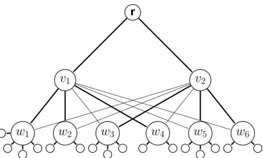
by those vertices and the vertices wi is made of 3m disjoint stars. See Figure 2.1 for a graph
representation of a 3-Partition instance with m = 2, B = 11 and D = {5, 3, 4, 3, 4, 3}. Notice that |V | = 1 + m + mB.
Solving RSpAF on G with β = B + 1 amounts to finding an arborescence where the size of the subarborescence rooted at each vj is smaller than or equal to B + 1. If there is a
solution to RSpAF on G, then, from the proof of Property 2.2.1, there is a solution S such that (r, vj) ∈ S ∀j = 1, ..., m, and each wi is connected to exactly one vj, otherwise
there is a cycle. Given a vertex v ∈ S, let S(v) be the subarborescence of S rooted at v: ∀j = 1, ..., m, we have |S(vj)| ≤ B + 1 and Pj=1,..,m|S(vj)| = |V \ {r}| = mB + m. Thus,
∀j = 1, ..., m, |S(vj)| = B + 1 and S(vj) contains vj and several vertices wi, each having
di− 1 successors in S. Finally, the constraints B/4 < di < B/2 imply that, ∀j = 1, ..., m, vj
that |S(wj1)| + |S(wj2)| + |S(wj3)| = |S(vj)| − 1 = B.
Then, it is easy to obtain a solution to the 3-Partition instance. For each j = 1, .., m, we set Mj = {|S(wj1)|, |S(wj2)|, |S(wj3)|} = {dj1, dj2, dj3}. We have m disjoint sets, each of size B, which cover exactly D. For the instance given in Figure 2.1, a solution to 3-Partition can be associated with the arborescence given in thick: M1 = {5, 3, 3} and M2 = {4, 4, 3}.
Moreover, from a solution to the 3-Partition instance, it is easy to obtain a solution S to RSpAF for the associated graph G, using similar arguments.
The 3-Partition problem is Complete in the strong sense, meaning that it remains NP-Complete even if the integers in D are bounded above by a polynomial in m. Thus, the reduction can be done in polynomial time and RSpAF, which is clearly in NP, is
NP-Complete. 2
RSpAF being NP-Complete, RSpA is NP-Hard, and so is RCStA because it is a gener-alization of RSpA. Let us now consider capacity constraints on the edges. RSpAF can be seen as a special case of the general capacitated spanning arborescence problem where the demand at each node is an integer (our demands are all equal to 1), and hence from Theorem 2.2.1 we obtain the following corollary:
Corollary 2.2.2 Given a graph G = (V, E, r, d, u) where d represents the (integral) demands at each node and u the capacities of the edges, the problem of deciding whether there exists a spanning arborescence of G, rooted at r and respecting the capacities, is NP-Complete (even if u is a uniform function and all demands are equal to 1).
This extends the following result due to Papadimitriou [49]: given two positive values C and K and a graph G = (V, E, r, c) where c is a cost function on the edges, the problem of deciding whether there exists a spanning arborescence S of G rooted at r, such that each subarborescence of S not containing r contains at most K vertices, and with total cost at most C, is NP-Complete.
The complexity results given in this section concern undirected graphs, and so the more general case of directed graphs too, since an undirected graph can be transformed into a directed one by replacing each edge by two opposite arcs. If we consider problems with ca-pacity constraints, we give the same caca-pacity to both opposite arcs: since we search for an
r
v
2v
1w
2w
1w
3w
4w
5w
6Figure 2.1 Graph and RSpAF solution resulting from the 3-Partition instance in which m = 2, B = 11, D = {5, 3, 4, 3, 4, 3}
arborescence, only one of them will appear in the solution.
In the following, we study the more general following problem, which is hence also NP-hard:
Robust Capacitated Steiner Arborescence problem (RCStA)
INSTANCE: A connected graph G = (V, E, r, T, u) with r ∈ V , T ⊆ V \ {r} and u a positive integer function on E.
PROBLEM: Find an arborescence S = (VS, AS) with VS ⊆ V and AS ⊆ E, rooted at r and
spanning the terminals of T , which respects the arc capacities and minimizes the number of terminals disconnected from r when an arc a is removed from AS, in the worst case.
2.3 Mathematical formulations and tests
In this section we propose formulations for robust Steiner problems where the robustness is considered either as a constraint with the objective of minimizing the cost, or as an objective with or without constraints on the cost. Moreover, we study two kinds of robustness by considering worst or average consequences of breakdowns.
set of terminals T , and capacity and cost functions, respectively denoted by u and c, on the arcs. As seen before, if G is undirected, then we replace each edge by two opposite arcs with the same capacity and cost. To formulate the different problems, for each arc (i, j) ∈ A we introduce the 0-1 variable yij and the integer variable xij, where yij equals 1 if and only if the
arc (i, j) is selected in the solution, and xij represents the number of terminals connected to
the root through the arc (i, j), or equivalently the number of terminals in the subarborescence rooted at j.
We introduce the following polyhedron T : T = x ∈ N|A|, y ∈ {0, 1}|A| P (i,j)∈A xij − P (j,k)∈A xjk = |T | if j = r −1 if j ∈ T 0 otherwise ∀j ∈ V P (i,j)∈A yij ≤ 1 ∀j ∈ V \ {r} xij ≤ uijyij ∀(i, j) ∈ A
In the following, we write (x, y) ∈ T when we consider a couple of variables verifying the constraints of T . The first set of constraints in T ensures both the conservation of the number of terminals connected through each Steiner vertex j ∈ V (flow conservation) and the connection of the root to all terminals. The second set of constraints ensures that the solution is an arborescence, i.e., that each vertex has at most one predecessor. Finally, the third set ensures that there is no flow on a non existing arc, and that the number of terminals connected through an arc (i, j) ∈ A does not exceed its capacity. In the following, the relative gap between two costs will be denoted by ∆. The well-known problem of the Capacitated Steiner Arborescence (CStA) can be formulated as follows [20]:
CStA min (x,y)∈T X (i,j)∈A cijyij
As explained previously, we evaluate the robustness of a Steiner tree by considering the number of terminals disconnected from the root in the worst scenario, that is, the maxi-mum number of terminals connected through an arc incident to the root, which is equal to maxj∈Γ+
G(r) xrj. Let R be a fixed bound on this value: we may disconnect at most R terminals
from the root by deleting an arc. We propose the following formulation for the Capacitated Steiner Arborescence with bounded robustness (CStAbounded−robust):
CStAbounded−robust min (x,y)∈T P (i,j)∈A cijyij s.t. xrj ≤ R ∀j ∈ Γ+(r)
is to minimize the cost of the solution. If a model uses another objective function, then its name will start by a given letter, e.g., R if we want to optimize the worst-case robustness. We propose the following formulation for RCStA:
RCStA min (x,y)∈T j∈Γmax+G(r) xrj
The max function is handled in our formulation with the addition of a variable η with η ≥ xrj ∀j ∈ Γ+G(r): the objective function is then to minimize η. Since this formulation
does not take the cost into account, we also propose a new formulation where we bound the cost of a solution by a given value C:
RCStAbounded−cost min (x,y)∈T j∈Γmax+G(r) xrj s.t. P (i,j)∈A cijyij ≤ C
The max function is handled in RCStAbounded−cost in the same way than in RCStA.
However, the previous models only consider the worst-case of a breakdown. It appears that it could also be interesting to "balance" the tree in order to reduce the loss due to an "average breakdown". To this end, we consider arc failures at each vertex and not only at the root, i.e., for each i ∈ V , we consider the worst case of a breakdown of an arc leaving i. This cor-responds, for each i ∈ V , to the maximum number of terminals that cannot be reached from the root in case of a breakdown of an arc (i, j), j ∈ Γ+G(i), or equivalently to the maximum flow on an arc (i, j), j ∈ Γ+G(i). We define the "balanced robustness" as the sum of these values: P
i∈V maxj∈Γ+G(i) xij. This function appears to be an alternative formulation of the
losses in both the worst and the average breakdown robustness.
We will use the letters BR to refer to models where one wants to optimize the balanced robustness. We propose formulations similar to the previous ones for the Capacitated Steiner Arborescence with bounded balanced robustness, where we bound the balanced robustness of a solution by a given value BR:
CStAbounded−balanced_robust min (x,y)∈T P (i,j)∈A cijyij s.t. P i∈V max j∈Γ+G(i) xij ≤ BR
The max function in the constraint is handled in CStAbounded−balanced_robustwith the addition
of |V | variables βi for each vertex i of V with βi ≥ xij ∀j ∈ Γ+G(i): the sum of the variables
βi with i ∈ V must then not exceed BR.
The following formulation aims at computing the best balanced robustness:
BRCStA min (x,y)∈T X i∈V max j∈Γ+G(i) xij
The max function is handled in BRCStA in a similar way than in CStAbounded−balanced_robust:
we minimize the sum of the variables βi instead of setting an upper bound to this sum.
Moreover, we can keep this latter objective while bounding both the worst-case robustness (by R) and the cost of the solution (by C). We obtain:
BRCStAbounded−robust−cost min (x,y)∈T P i∈V max j∈Γ+G(i) xij s.t. xrj ≤ R ∀j ∈ Γ+G(i) P (i,j)∈A cijyij ≤ C
The max function in the objective function of BRCStAbounded−robust−cost is handled in the
same way than in BRCStA.
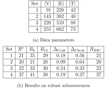
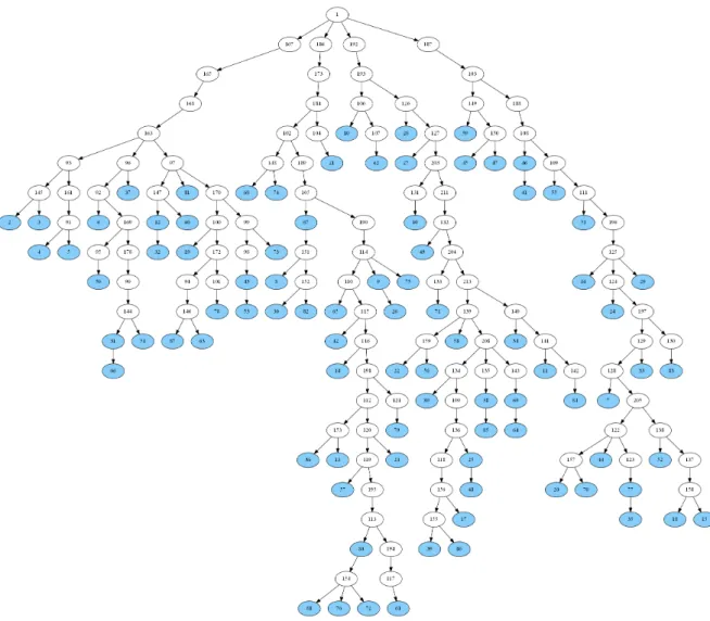
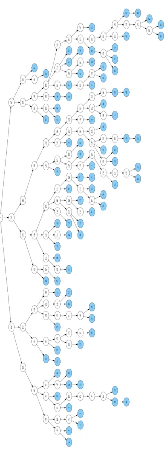
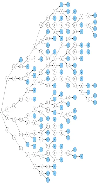
We tested those formulations on real wind farm data sets. Even if the number of instances is small, the results are interesting to analyze, and we can compare the robustness, costs and structures of the solutions. Data parameters and results are available respectively in Tables 2.1a and 2.1b. Figures 2.2, 2.3, 2.4 and 2.5 allow to visually compare the arborescences ob-tained according to the different models for the fourth data set (the filled circles correspond to terminals).
Figure 2.2 gives an optimal (non robust) capacitated Steiner arborescence (optimal solution of CStA); let us denote its cost by C∗. This arborescence cannot be qualified as robust since, in the worst case, all terminals can be disconnected by deleting the only arc incident to the root. Furthermore, the tree has a large depth, and hence the balanced robustness is not good either. This proves the importance of searching for a more robust solution. We consider first the worst case, RCStA, and we denote by R∗ the best robustness, i.e., the minimum value of the loss of terminals in the worst case of a single arc deletion. See Figure 2.3 for the associated solution on the test instance. Then, to obtain the minimum cost of a most robust solution, denoted by CR∗∗, we solve CStAbounded−robust with R = R∗: notice that the constraint is saturated in any feasible solution. Then, ∆Crob= (CR∗∗− C∗)/C∗ represents the "cost of robustness", i.e., the percentage of augmentation of the cost to get a robust solution.
In the same way, let BR∗ be the best balanced robustness (optimal value of BRCStA, not given in the table); see Figure 2.4 for the associated solution on the test instance. The cost of a solution with the best balanced robustness, denoted by CBR∗ ∗, is obtained by solving CStAbounded−balanced_robust with BR = BR∗, and ∆Cbrob = (CBR∗ ∗ − C∗)/C∗ represents the "cost of balanced robustness", i.e., the percentage of augmentation of the cost of a non robust arborescence to get a balanced robust solution.
We also study the behavior of the robustness when we bound the cost to a value close to the one of an optimal non robust arborescence : R8 (resp. R12) corresponds to the optimal value
of RCStAbounded−cost with a bound C = 1.08C∗ (resp. C = 1.12C∗).
We now analyze the results. The cost of robustness is quite variable on those instances (from 9 to 24%) but remains rather low. On the contrary, we can see that the optimization of the average robustness is way more expensive (raise from 33% to 64% of the cost) because it involves significantly more edges (see Figure 2.4).
As we can see on Table 2.1b, a cost augmentation of 8% or 12% on the optimal cost can result in a solution with a good value of worst-case robustness for some instances: instances 2 and 4 present an excellent value of such robustness with only a cost augmentation of 8%, while instances 1 and 3 have a rather good one with a cost augmentation of 12%.
Finally, we compare the optimal robustness R∗ to the robustness of the balanced arbores-cence Sb obtained by solving BRCStA, i.e., we compute in Sb (see Figure 2.4) the maximum
number of terminals which are disconnected after the deletion of an arc incident to the root. Let RBR∗ be this number, shown in the last column of Table 2.1b. For the test instances, the values of R∗ and RBR∗ are the same, which means that Sb is a good solution for both the worst and balanced robustness, but we have seen before that its cost is high. Indeed, for these instances, we see that forcing a solution with R = R∗ to be optimally balanced increases the cost by at least 33 %. Nevertheless, there is no guarantee in the general case that the best balanced solution also has the best robustness in the worst case, although the arcs incident to the root are involved in the computation of the balanced robustness.
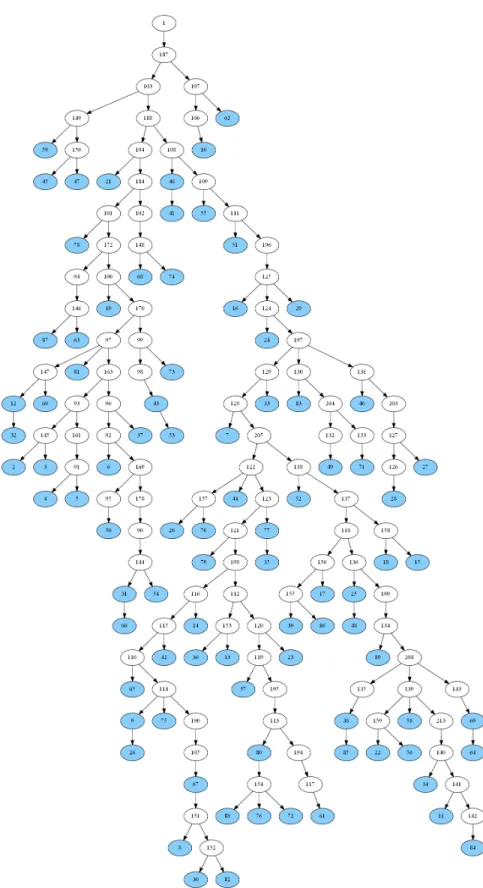
Table 2.1 Results on robust arborescences and data parameters Set |V| |E| |T|
1 91 220 42
2 143 382 40 3 220 510 88 4 255 662 73
(a) Data parameters
Set R∗ R8 R12 ∆Crob ∆Cbrob RBR∗
1 21 35 29 0.18 0.56 21
2 20 21 20 0.09 0.64 20
3 22 32 30 0.24 0.33 22
4 37 41 38 0.19 0.37 37
(b) Results on robust arborescences
When trying to minimize the number of disconnected terminals in the worst case (see RC-StA in Figure 2.3), we have seen that the associated solutions have a reasonable cost, but the average robustness is not good, since the tree remains too deep. When finding the Bal-anced Steiner arborescence (see BRCStA in Figure 2.4), the balBal-anced robustness is optimal and the robustness in the worst case is fine, but the cost can be really high (a raise of the optimal cost to 64% on those data sets). Adding bounds on both cost and worst-case ro-bustness, while minimizing the balanced robustness (see BRCStAbounded−robust−cost in Figure
2.5), yields a solution which has both a reasonable cost and a really good worst-case and balanced robustness, and hence it seems that it actually yields the best compromise between the three optimization criteria (the cost and the two types of robustness considered here).