Université Paris I Sorbonne
Master 2 Recherche Economie de la Mondialisation
UFR de sciences économiques 02
Power outages and the decision of under-grid
households to connect to the grid
2016
Présenté et soutenu par : Arnaud Millien
Directeur de soutenance : Jean-Claude Berthélémy
The University of Paris 1 Panthéon-Sorbonne neither approves nor disapproves of the opinions expressed in this dissertation: they should be considered as the author’s own.
L’université de Paris 1 Panthéon-Sorbonne n’entend donner aucune approbation ni désapprobation aux opinions émises dans ce mémoire: elles doivent être considérées comme propre à leur auteur.
Power outages and the decision of under-grid households to connect to the grid
Arnaud Millien*
* Centre d’Economie de la Sorbonne, Université Paris 1, 106 Blvd de l’Hôpital, 75013 Paris, France
Abstract
A low power reliability is challenging the electrical grid’s extension cost because it’s lowering the number of connected households. The quality effect is at least 5% higher than the wealth effect, eventually up to 47%, and emerges as the main hurdle to households’ connection.
Addressing the challenge of electrical outages would accelerate per se the annual number of new subscribers to the electricity distributor. The intermediate wealthy households would be the more prone to subscribe, provided that the availability of the power would be enhanced. The policy maker should be advised to put a peculiar effort on the technical features that sustain the reliability of power until its final destination.
Keywords : electricity, outages, lightning, grid, transmission and distribution lines, Kenya, poverty, instrumental variable
JEL : Q4, QO1, O18, O55, C26, C52
Acknowledgments
The author thanks Jean-Claude Berthelemy for his driving insights, Sandra Poncet and the teaching team of Maison des Sciences Economiques for their professional research advices, Afrobarometer that provided the data, Victor Béguerie for his advice on the poverty index, Olivier Santoni for supplementing the geographical data, Chris Davis for providing the support in using Enipedia and his fellow students for their good mood.
Introduction
In 2014, 620 million people had no access to electricity in Africa (IEA, 2014). Even connected firms and households suffer sever outages: for instance, 6.3 outages per months occurs in Kenya, each lasting 5.6 hours.1 The erratic volatility harms the firm’s production, while households are exposed to multiple adverse consequences on security, health,
education, and employment holding back the human capital accumulation.
In 2012, India suffered the most serious outage ever occurred: a national blackout paralyzed 670 million people for 48 hours. Balancing the response of supply to the volatility of demand is especially fragile, since electricity does hardly store. The ability to permanently supply the maximum consumption (peak-load) is defined as the reliability (NERC, 2011).
This article assesses the impact of reliability on the households’ decision to subscribe to electricity. It’s related with the stake of the grid’s extension cost in a poverty context. High costs of production and distribution yields heavy billing; meanwhile the lack of capacities makes the occurrence of outages more frequent. Facing both unaffordable
connection’s cost and unreliable service, the households might be reluctant to subscribe, what lengthens the break-even of new investments and deters in turn the settlement of new
capacities or transportation facilities. It looks hard to determine the right starting point for the low-income countries to escape from such a vicious cycle, between the lack of capacities and the lack of subscriptions.
Keeping a full reliability with insufficient capacities is moreover complicated in a growing population context, due to the increasing peak-load. High costs and long delays to build new infrastructures makes the supply’s growth slowly responsive, while the grid’s extension investments ought to be amortized fast enough by a large number of subscriptions. The households offer the widest customer potential, provided that they pay the monthly fees. So far, the electricity development has hardly been seen as a priority and the aforementioned issues have been frequently solved by a supply’s shortage. But new context’s elements are changing the challenges/opportunities balance for Africa, like the strongly decreasing production’s cost of renewable energy, the fast equipment’s rate of households in mobile
phones, sustaining more regular m-payments and the inclusion of the reliable access to energy for all as the 8th Sustainable Development Goal in 2015.
Kenya is facing such a contrasted evolution. Between 2009 and 2014 the population grew by +14%, while the connected households grew by +218%. As a result, the peak-load grew by +41% as well as the amount of installed capacities (Annex 1). But the production of
electricity is costly, scaling from 0.14$ up to 0.25$ for diesel plants, and outages are severe: in 2014, 9% of the households report a full unavailability of the power, and 20% report only occasional availability (Afrobarometer, 2014). In recent years, the grid has been extended, reaching a coverage rate over 80% in 2/3 of the counties (Afrobarometer, 2014). But the lack of connections is pushing up the distribution’s marginal cost : evidenced by (Lee et al., 2014), if all the buildings within the distribution’s radius of a transformer (600 m) were connected, the median investment per connection would be $210 instead of currently $ 2,427. However, as shown above, the growth of the customers’ number is much faster than the one of the peak-load, opening opportunities to positively address the challenge of the households’ connection: their impact on the grid could be not so heavy while conversely, enhancing the distributed reliability could possibly accelerate the households’ subscription, hence reducing the cost of the grid’s extension.
Isolating the causal impact of outages on the connections’ level faces the risk of a reverse causality. In addition, it is not obvious to disentangle the time dimension of the reliability from its geographical impact on the connections to the grid.
Relying on (Andersen and Dalgaard, 2013), this article uses the lightning intensity as an instrument that has proven to be efficient to solve this peculiar risk, extending meanwhile the previous work at individual level. It also introduces a poverty index in order to compare the impact of the outages to the one of poverty on the connection’s level. Exploiting the large share of natural endowments in the Kenyan energy mix, this article introduces the districts’ distance to the closest electrical generator as an additional instrument for the outages, under the assumption of a homogenous grid.
The Afrobarometer survey 2014 provides cross-sectional data on the households’ assets and their individual exposure to electrical outages in Kenya. The lightning data are sourced from the LIS/OTD Gridded Climatology dataset. The location of to the plants comes from
Enipedia, a collaborative database.2 From the first, an individual synthetic index of poverty is
computed for each household, as well as the average exposure to outages within a district. From the two others, lightning and distance to the closest plant are aggregated at district level. This article brings the causal evidence by resorting to lightning as an instrumental variable. Under equatorial latitude, Kenya lays among the most exposed countries to storms in the world, with a lightning’s intensity 9 times higher than in France. Compared to other Sub-Saharan countries, Kenya also exhibits a strong heterogeneity of lightning. Intensity and heterogeneity makes the variable a good candidate to instrument the outages, as also suggested by (Map 1).
Map 1: LIGHTNING AND OUTAGES BY COUNTIES
Source : (Afrobarometer, 2014)
Lightning is an external random phenomenon that can causes a variety of direct damages on the electric pylons: thermic, mechanical or electrical shocks. When damaging the grid, it has a strong zone effect making its correlation with the outages much higher than the scarce
possibility to damage individual junction’s nodes. Thus, it might be correlated with the connections’ level only through its own correlation with the outages’ occurrence.
To disentangle the past effect of the reliability on the connections’ level, this article uses a cluster estimation combined with the assumption of a homogenous grid. In absence of any bottleneck, the outages suffered in a district might solely but strongly depends on its distance to the closest generator, modulo the capacity of the plant.
Outages have a significant negative impact on the households’ decision to subscribe to electricity: on average, 1 percent point lower reliability in a median district triggers 0.67 percent point less connections. The role of outages in this decision is on average 26% higher
22.3 - 42.6 (11) 4.1 - 22.3 (13) 2.3 - 4.1 (11) 0.8 - 2.3 (12)
Source : Data from Afrobarometer 2014
Lightning's intensity by counties
0.50 - 1.00 (10) 0.25 - 0.50 (10) 0.13 - 0.25 (11) 0.00 - 0.13 (11) No data (5)
Source : Data from Afrobarometer 2014
than the one of poverty, from at least 5% in the most conservative estimation in a median district, up to 47% in the wealthiest districts.
The level of outages itself impacts the households’ sensitivity. Where the rate of outages is “only” 30%, 1 percent point upgrade of reliability would trigger 1.09 percent point more connections. Where the outages’ frequency is too high, the wealth or poverty level of the households has no more effect: they are only responsive to the too low reliability. Conversely, in the poorest western regions of Kenya, the households are not sensitive to outages.
The low reliability has the maximum deterring impact among the households with
intermediate wealth, who are the most reluctant to subscribe in presence of outages. For 1 percent point higher reliability, the intermediate wealthy households would be connected 1.28 percent point more.
The remainder of the article is organized as follows. Section I describes the context of the electrification in Kenya. Section II reviews the literature at the starting point of this study. Section III exhibits the data and their origin. Section IV addresses the identification strategy, then section V explains the diagnosis methodology and shows the results, while section VI deals with robustness checks. Finally section VII proposes an extension of the model and section VIII concludes with policy implications and possible advices.
I - Context and issues of electrification in Kenya
The electrical sector in Kenya is organized with a central distributor (KPLC) under a PPP mandate, a public grid manager (KETRACO) and a set of producers, composed by KENGEN, a majority government owned company that produces over 85% of the capacity, and
Independent Power Producers (IPP) (Annex 2). A state-owned Special Purpose Vehicle is dedicated to the development of geothermal production (GDC). The Rural Electrification Authority (REA) is a state agency that has launched the Last Mile Connectivity project in September 2015, addressing the issue of unconnected under-grid households in rural areas. As at 2014, electricity produced from the country’s natural endowments represents 56% of the capacities (Graph 1, left), with a large share from geothermal origin (19,1%), still growing in 2015 (26,6%). Kenya owns the largest geothermal single plant of the world in Olkaria IV (140 MW), the geothermal industry producing the cheapest electricity of the country: between 0.03$/KWh and 0.14$/KWh, the most expensive geothermal plant produces at the same cost as the cheapest diesel plant. The flagship projects in 2016 are the on-going construction of a new geothermal site in Menengai (105 MW ; further 360 MW planned) and the kick-off of a
large wind production project close to Lake Turkana (320 MW) (Davis et al., 2015). Two solar plants projects are engaged in Eldoret (2x40 MW, PPA signed) and in Garissa (55 MW).
Graph 1 : PRODUCTION'S CAPACITY BY FUEL TYPE
KPLC had 2 million customers in 2012, 2,7 million in 2014 and should reach 4,3 million in 2016 (KPLC, 2015). The fast growing customer base could be a risk for the reliability, as the electricity crisis in California has illustrated it in the 90’s.3 Facing a growing peak load while lacking capacities, KPLC is planning outages to avoid the worst scenario of a national
blackout.4 A recurrent debate in Kenya points out the distribution’s trade-off between firms and households. The historical choice has been to prioritize the reliability for the firms, in order to not deter the foreign investors to operate in Kenya.
But too frequent outages could make the households reluctant to subscribe, for the cost of the service appears too high given its erratic availability. While the grid has been extended most all over the country, the connection’s rate remains below 50% in half of the counties (Map 2).
Map 2: COVERAGE’S RATE AND CONNECTION’S RATE
Source : (Afrobarometer, 2014) 3http://www.eia.gov/electricity/policies/legislation/california/subsequentevents.html 4http://kplc.co.ke/category/view/50/power-interruptions 2.6% 19.1% 33.9% 44.0% 0.3% Bio Geothermal Hydro Thermal Wind
Source: Enipedia and Author's contribution
Graph (1) - Production's Capacity by fuel type
74.6% 25.4%
Natural Driven Location Thermal, not Coastal located
Source: Enipedia and Author's compilation
Graph (1) - Production's Capacity by fuel type
0.88 - 1.00 (22) 0.67 - 0.88 (12) 0.00 - 0.67 (13)
Source : Data from Afrobarometer 2014
Coverage's rate by counties
0.56 - 0.94 (10) 0.43 - 0.56 (11) 0.22 - 0.43 (11) 0.00 - 0.22 (11) No data (4)
Source : Data from Afrobarometer 2014
As evidenced by (Lee et al., 2014) the lack of connections multiplies the marginal cost of the grid’s extension by ten. Therefore, the Last Mile Connectivity project entails a special effort for the poorest households, dropping down the fee of connection from KSh35,000 to
KSh15,000 (REA, 2015). However, this action plan entails the underlying assumption of an exogenous quality supply. If there is a specific sensitivity to the power reliability, addressing the solely financial issue might not be enough. In other words, would a better power reliability raise the connections’ level quicker than the wealth’s growth of the households?
II - Related literature
This paper is related with a first strand of literature that has studied the role of the grid’s quality on the households’ connection. Two factors have been identified, the density of the transmission lines and the proximity to the distribution’s transformers. The frequency of outages is commonly used as a measure of the service’s quality.
With a panel of 10,000 households from the IHDS database in India (Chakravorty et al., 2014) have shown that the density of the transmission lines facilitates the decision to connect : from an initial level, increasing the density of the cables by one unit increases the grid’s connections by 10 percent points. From the Indian case, (Khandker et al., 2014) has also identified the role of transmission and distribution losses on lines.
With a large dataset on geo-tagged structures and residential compounds in Kenya (Lee et al., 2014) have studied the role of the proximity to the closest transformer, distinguishing the access to electricity in a geographical unit from the households’ connection. Their work disentangles the impact of the grid’s extension from the individual proximity to access nodes. Being the first to introduce the notion of “under-grid” households, they have brought
evidences that the wealth effect outweighs the distance to the connection node: within 200 meters, the probability of connection decreases by 20% for the poorest households, who are identified by the walls’ quality of the building where they live.5
Using the IHDS survey of 2005 (Khandker et al., 2014) have shown that the decision of Indian households to connect to the grid depends both negatively on the price and positively on the quality of the power : an additional available hour of power increases the adoption rate by 2.7%. Villages without power outages have a higher households’ access rate (81%) than those with more than 20 hours of outages per day (38%).
As a second strand of literature, the seminal work of (Andersen and Dalgaard, 2013) has brought lightning as an efficient instrumentation to isolate the causal effect of outages on the growth rate, with macroeconomic data on Africa. An increase of + 2.3 outages per month reduces the growth by 1.5 points. Applied to Kenyan data in 2013, such a fail on quality would cost 800 million dollars per year.6
This paper aims to extend their work in several ways: first, the study will focus on Kenya, one of the country of their Sub-Saharan sample; second, it will use individual data on households; therefore, it will relate their work with the first strand of literature by studying the outages’ impact on the connection’s probability. Finally, it will extend the specification, controlling for the poverty level and expanding the set of lightning-based instruments.
This study also relies on the first strand of literature in the following dimensions. First, it will encompass the notion of “under-grid” households, extending the work of (Lee et al., 2014) at the smallest granularity level. Second, while evaluating the impact of the distance to the transformer, (Lee et al., 2014) makes the underlying assumption of an exogenous quality supply, uniform in time or space. This study exploits the heterogeneity of outages between districts to disentangle the specific impact of those last on the connection’s decision. Third, while the distance to the transmission lines could be endogenous to the grid’s extension, using the lightning intensity as in (Andersen and Dalgaard, 2013) should provide a strong
exogenous instrument, independent of the initial electrification level (Chakravorty et al., 2014). Fourth, the study gets one step backward in the causal chain studied by (Khandker et al., 2014): while they instrument the access to electricity as a factor of electrification’s benefits, this study intents to establish the causal impact of outages on the connection’s decision. Fifth and finally, as (Lee et al., 2014) and (Chakravorty et al., 2014) have suggested the strong role of the distance, respectively to the distribution or to the transmission lines, this study intents to exploit the distance to the generators as an additional instrument.
A third dimension of the literature evaluates the benefits of the electrification for the connected households. (Khandker et al., 2014) have found a reduction of -3.3 hours in the monthly time devoted to the collection of biomass thanks to the reduction of the marginal cost of the lumen. Therefore, electrification has increased the schooling’s rate and duration. It has also reduced the consumption of kerosene used in oil lamps by -35%, a major health risk factor. As for the activity outcomes, the access to electricity has contributed to increase the
employment’s rate of women by + 1.5% and + 17% for that of men, while (Chakravorty et al., 2014) have measured an increase in non-agricultural income by +9%. This study will focus on the interaction effect between outages and poverty on the connection’s decision.
III - Data
The data on electrical coverage, connections and outages are provided by the Afrobarometer survey on Kenya, from the questionnaire 2014, round 6. The database contains 2,397 cross-sectional observations on households, segmented by the geographical administrative units of Kenya, counties and districts. The analysis is based on the 1,989 respondent households living in a unit with access to electricity.
The access to electricity is known from the descriptive part of the questionnaire filled by the interviewer. A specific question provides the information on the reliability of the power, with five distinct levels of availability (1 : never, 2 : occasionally, 3 : half the time, 4 : most of the time, 5 : all the time). Since the question also asks to the household whether it owns an electrical connection (0 : no electric supply), there might have been some inconsistent answers with the descriptive part filled by the interviewer. Specific filters have been applied for the computation of the outages’ rate (see section IV) to make them consistent.
The lightning intensity is sourced from the LIS/OTD dataset that collects the number of lightning’s impacts within 50km² squares. They have been averaged by districts on the 1995-2013 period. Climate controls (altitude, temperature and precipitation) are provided by the geographical database of the FERDI, as well as the distance to Mombasa, weighted by the road’s quality. The localization of the generators is provided by the Delft University from its Enipedia collaborative database where the capacity has been supplemented by the author’s researches.
IV - Identification strategy
Objective and main specification
This study aims to disentangle the specific impact of outages on connections by first isolating the quality effect, second comparing its magnitude with the wealth effect and third exploring the interaction of both variables.
The general equation below considers the effect of outages (CO) on households’ connection (connection) to the electrical grid. The main variable that could also determine their decision is obviously their wealth that the model ought to control for. To this end, one uses the data on
the households’ assets from the Afrobarometer 2014 survey, to compute a composite poverty index (pov_index). The potential cross-effect is captured by introducing an interaction term between the outages and the poverty index. Extending the parsimonious specification of (Andersen and Dalgaard, 2013), one considers the general regression model :
𝐶𝑜𝑛𝑛𝑒𝑐𝑡𝑖𝑜𝑛𝑖 = 𝑎0+ a1. 𝐶𝑂𝑢(𝑞) + a2. 𝑝𝑜𝑣_𝑖𝑛𝑑𝑒𝑥𝑖+ a3. 𝐶𝑂𝑢(𝑞)𝑥 𝑝𝑜𝑣_𝑖𝑛𝑑𝑒𝑥𝑖+ ui where, i is the household, u is the district and q is the severity level of the outages.
Variables definitions Dependent variable
The dependent variable (connection) is a dummy that equals 1 for a connected household living in a district with access to electricity. The evaluation exploits the geographical
heterogeneity of the connection’s rate, spreading from 94% in Nairobi to 0% in Lamu or 4% in Homa Bay.
Poverty index
As in (Booysen et al., 2008), the poverty index is derived from an MCA of the unconnected assets owned by the household (Table 1). It’s the linear combination of the standardized coordinates of the categories on the first axis, weighted by their contribution. It’s computed for each household, with positive values for the poorest one.
Table 1 : ACTIVE VARIABLES IN THE MCA
The first axis concentrates 54% of the inertia, while the second axis (21%) and the third axis (3,3%) are largely built from missing values of any peculiar categories. Hence, the first axis captures all the meaningful information on the poverty level and can be used confidently as a synthetic composite index. Annex 3 exhibits the main components that contribute positively and negatively to the first axis.
Power reliability index
The power reliability index CO(q) is defined by the rate of cumulative outages (CO) at successive levels of severity (q) in a geographical unit. In a first step, the simple rate of
Q91a. Own radio radio
Q91c. Own motor vehicle, car or motorcycle motor
Q91d. Own mobile phone mobile
Q92a. How often use a mobile phone use_mobile
Q93a. Source of water for household use water
Q93b. Location of toilet or latrine sanit
Q104. Type of shelter of respondent shelter
outages qualifies four severity levels (1 : total, 2 : serious, 3 : partial, 4 : occasional). In a second step, the power reliability index is the rate of cumulated outages for a given severity level. For the sake of simplicity, the same qualification will be used in the study to qualify the cumulated outages; for instance, the accumulation of outages from total to partial frequency will be denominated “partial” severity (Table 2).
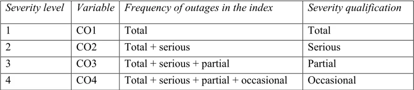
Table 2 : POWER RELIABILITY INDEXES BY SEVERITY LEVEL7
Severity level Variable Frequency of outages in the index Severity qualification
1 CO1 Total Total
2 CO2 Total + serious Serious
3 CO3 Total + serious + partial Partial
4 CO4 Total + serious + partial + occasional Occasional A large part of the empirical work will be dedicated to assess the most relevant level of severity in order to estimate the outages’ effect on the households’ connection.
Due to the low number of observations, some districts report only one connected household. In that case, the observed rate of outage is 100%, at the severity level answered by the
household. A filter has been set to keep only the units with at least two connected households.
Neighboring effect
In a context of high connection’s cost and low reliability of the power, subscribing to
electricity might also depend on the example of the neighbors, sustaining a diffusion or barrier process. The observed level of connections in 2014 might actually result from a past diffusion or inertia among the households within a unit: it might be much higher in a district than in another one because households have been encouraging each another to subscribe in the first (diffusion) while they have been seeking for mutual confirmation bias to not subscribe in the last (barrier). As identified by (Lee et al., 2014), positive externalities might also be at work, due to economies of scale in the interconnected electrical network.
7 As pointed out by (Chakravorty et al., 2014), the word « reliability » has a precise definition in electrical
engineering -as defined by (NERC, 2011)- a reason why they prefer to use the term “quality”. However, as clearly stated in the aforementioned reference, the purpose of the standard definition of reliability is “to maintain
interconnection steady-state frequency within defined limits by balancing real power demand and supply in real-time”. Whether random or planned, outages are clearly a severe breach of the standard definition. From an
economic perspective, their occurrence can be used as a synthetic index of this violation to balance supply and demand.
Therefore, the assumption of i.i.d observations can’t be hold, leading conversely to assume heteroscedasticity within the units. The neighboring effect will be captured by clustering all the estimations, following (Chakravorty et al., 2014) and (Khandker et al., 2014).
Since the model mixes an individual level variable (the poverty index) and an aggregated variable (the power reliability index), resorting to clusters also solves the Moulton bias (Moulton, 1990). Computing the variance-covariance matrix by clusters corrects the under-estimation of the standard error that would otherwise results from using an aggregated variable. The significance of the coefficients can be then properly diagnosed.
Gradual estimation’s Methods
The model will be first estimated by an OLS at districts’ level to identify the effect. In the next step, using instrumental variables ought to solve the endogeneity risks. A Probit specification should be then appropriate to estimate the probability of connection and it will also be instrumented. Finally, an extension will be conducted to capture the effect of the next level’s severity.
Endogeneity issues and Instrumentation
The evaluation must deal with three econometric risks of endogeneity. First, there is a risk of reverse causality because the growing number of connected households could be itself a cause of outages (see section I). Second, the data are sourced from a field questionnaire and might be distorted by a measurement error.
Third, a major determinant of the connections’ level could have been omitted in the
specification. The literature suggests three main hurdles (Khandker et al., 2014), (Lee et al., 2014): the high connection’s cost, the poor-quality of the building and the unreliability of the service. Since the first barrier is a matter of relative wealth, the poverty index is a suitable proxy. As this last entails the type of shelter, it captures also the second potential omitted variable and can be thus used as a proxy to control for both hurdles together. However, the index being built from an MCA, a robustness check should test for any residual correlation of the shelter’s type with the error term. The third hurdle is the effect addressed by this study. The distance to the closest electrical transformer might also modify the ability to connect to the grid (Lee et al., 2014). This issue is addressed by combining the clustering approach with the sampling delimitation to under-grid households, in districts with access to electricity. Yet there might be forgotten or unknown, even minor, omitted variables. The only way to deal simultaneously with the three risks of endogeneity is to resort to an instrumental variable.
KPLC identifies seven causes of outages: extreme weather conditions (wind, lightning, rain, floods), contacts of animals with the lines or transformers, growth or fall of the trees, vehicle collisions, vandalism, aging equipment and planned interruptions.8 From the detailed
qualitative assessment in Annex 4, wind, rain and floods would not meet the exclusion restriction due to their strong zone effect. Animals’ contacts, trees’ growth and vehicle collisions would easily meet the exclusion restriction, though only providing weak
instruments. Vandalism is obviously endogenous to poverty and would thus not be correlated to lower connections only through outages. The age of installations is by definition not random, hence not an exogenous factor.
Finally, only the lightning meets the three requested properties for an instrumentation, being purely random, strongly correlated with the outages’ occurrence while acceptably not a direct cause of lower individual connections (see Annex 4). The evaluation exploits the strong heterogeneity of lighting in Kenya, among the highest of the world in the western mountainous provinces while comparable to European level in the eastern regions.
A potential reverse tide effect has also been identified (Annex 4): a power shortage can cause a sudden over-load along the electrical wires that could in turn trigger new outages in the neighbor districts. It is thus necessary to instrument the outages also by the lightning intensity in the surrounding districts.
A third instrument is introduced with the distance of the district’s centroid to the closest generator, inversely weighted by the capacity of this last. The lack of capacities feeding the grid plays a key role in the outages’ occurrence. Under the assumption of a homogenous grid without any bottleneck, ie with technical features everywhere of the same quality, the ability of KETRACO to saturate it depends solely on the amount of produced electricity. On another hand, the received reliability in connected inhabitations depends in time on the discrepancy between demand and power supply. At a fixed point in time and under the homogenous grid assumption, the outages suffered in a district might solely but strongly depend on its distance to the closest generator, modulo the capacity of the plant.
(Lee et al., 2014) have used the distance to the closest transformer to explain the connection’s probability while this study is looking for an instrument of outages. Being at the termination of the grid for the last mile distribution, the transformers are fed by the lines’ network and
might undergo themselves the consequence of an upstream tension fall. The two distances play different roles.
The distance to the closest generator meets the instrumentation’s requirements because (1) it is both an external and random parameter from the outages, since the plants’ location is related with the country’s natural endowment (volcano, rivers, lakes, wind and Mombasa harbor on the coast) : as shown in (Graph 1), such plants account for 3/4 of the installed capacities ; (2) the distance to the plant has no influence per se on the connection’s decision. If the households were to subscribe more because being close to a plant they expect less outages, it is exactly what the instrument ought to captures.
It is computed as the minimum distance among all the generators, weighted by the inverse of the capacity of the closest generator over the total capacity of production. It can be seen as a proxy for the electricity equipment’s rate of the district.
V - Empirical diagnosis and results
Assessment methodology
The models are organized in four classes, introducing gradually the effects to be assessed (Annex 5). The first three classes are denominated “foundation” while the fourth is denominated “extension”, to be used in section VII. In the foundation assessment, four models per class are defined, given the severity level. The three classes gather 12 models that are presented together for the diagnosis. This last compares the models in order to qualify the best estimation, using the appropriate statistical tests for the estimation’s method.
The decision criteria are based on a backward-reading of the tests : the main objective is targeted first, then one checks that the previous test was passed successfully, the
antepenultimate also, and so on, until all the tests compounding the decision chain are met. If a test fails, while the first steps were met, one switches to the closest model that met the same initial tests in the decision-chain.
Entry model : OLS at district level
Table 3 shows the assessment of a simple OLS method applied to the three classes base, ctr and i. The backward decision criteria are the lowest AIC (column 6) and the lowest p-value for the Student test of the cumulative outages (column 4). The lowest AIC (1947) leads to retain the model iCO3_reg, where the p-value of CO(3) equals 0.000.
Table 3 : ASSESSMENT OF THE OLS MODELS AT DISTRICTS LEVEL
In this simple LPM specification (Table 4, column1) both the cumulative outages at partial severity level and the poverty index have a negative coefficient, significant at 0.1% level. Their interaction is also significant, at 1% level. The number of clusters (90) ensures that the standard error converge to its true value, leading to a proper assessment of the estimates’ significance (see Annex 6). From the standardized regression, one standard deviation of outages has an impact around the half (-0.099) of the one of poverty (-0.199).
Table 4 : LPM OF CONNECTIONS AT DISTRICTS LEVEL
This finding is an important result since it confirms the sign found by (Andersen and
Dalgaard, 2013) for Sub-Saharan countries as a whole. Their result still holds for Kenya with detailed data on households, opening avenues for field’s applications.
The LPM estimation yields accurate estimates, but inconsistent due to the endogeneity issues. As remarkable in Table 3, the coefficient of outages is downward biased in the Base
specification (-0.515) compared to the one in the ctr specification (-0.313): the poverty index dCO3_reg -0.465 0.126 0.000 23.5 1944 1669 90 dCO2_reg -0.377 0.079 0.000 23.4 1946 1669 90 dCO1_reg -0.386 0.098 0.000 23.3 1949 1669 90 iCO4_reg -0.357 0.138 0.011 21.6 1984 1669 90 iCO3_reg -0.362 0.070 0.000 23.3 1947 1669 90 iCO2_reg -0.361 0.077 0.000 22.6 1962 1669 90 iCO1_reg -0.419 0.117 0.001 21.7 1982 1669 90 ctr_CO4_reg -0.339 0.131 0.011 21.5 1985 1669 90 ctr_CO3_reg -0.313 0.069 0.000 22.8 1957 1669 90 ctr_CO2_reg -0.273 0.077 0.001 21.8 1979 1669 90 ctr_CO1_reg -0.142 0.103 0.171 20.2 2014 1669 90 base_CO4_reg -0.591 0.165 0.001 5.1 2302 1669 90 base_CO3_reg -0.515 0.068 0.000 8.4 2242 1669 90 base_CO2_reg -0.471 0.072 0.000 5.9 2286 1669 90 base_CO1_reg -0.413 0.101 0.000 2.1 2354 1669 90 Model (1) Outages (2) Std Error (3) P value (4) Adj. R2 (5) AIC (6) N (7) Nb Clusters (8) * p<0.05, ** p<0.01, *** p<0.001 _________________________________________________________________ Variance : Delta-method delta by Average marginal effects. SE in parentheses. LHS : Adj. R² 0.23 0.23 Nb Cluster 90 90 N 1669 1669 (0.036) (0.028) Constant 0.637*** 0.501*** (0.015) zpov_idx -0.199*** (0.018) c.zCO3#c.zpov_idx 0.051** (0.020) zCO3 -0.099*** (0.070) pov_index -0.735*** (0.184) c.CO3#c.pov_index 0.512** (0.070) CO3 -0.362*** Unit values Standardized values
would be an omitted variable if not taken in account. The study now turns to assess empirically the instrumentation choice.
Neutralizing the endogeneity risks: assessing the instrumentation quality Assessment criteria
Table 5 below describes the backward-ordered tests to assess the relevant severity level in the 2SLS method. Annex 13 exhibits their technical application more in depth.
Table 5 : BACKWARD DECISION-CHAIN ON THE INSTRUMENTATION’S QUALITY
Question Test
Are the instruments strong enough? Stock-Yogo < 30 F > 6 with p < 1% Are the estimates of the outages significant,
even if the instrument were to be weak?
Anderson-Rubin test (p <1%) Is the model correctly identified? Endogeneity test (p < 5%)
Under-identification test (p < 5%)
Over-identification Hansen test (p > 10%) Does the instrumentation bring a significant
difference in estimates?
Hausman test (p < 5%)
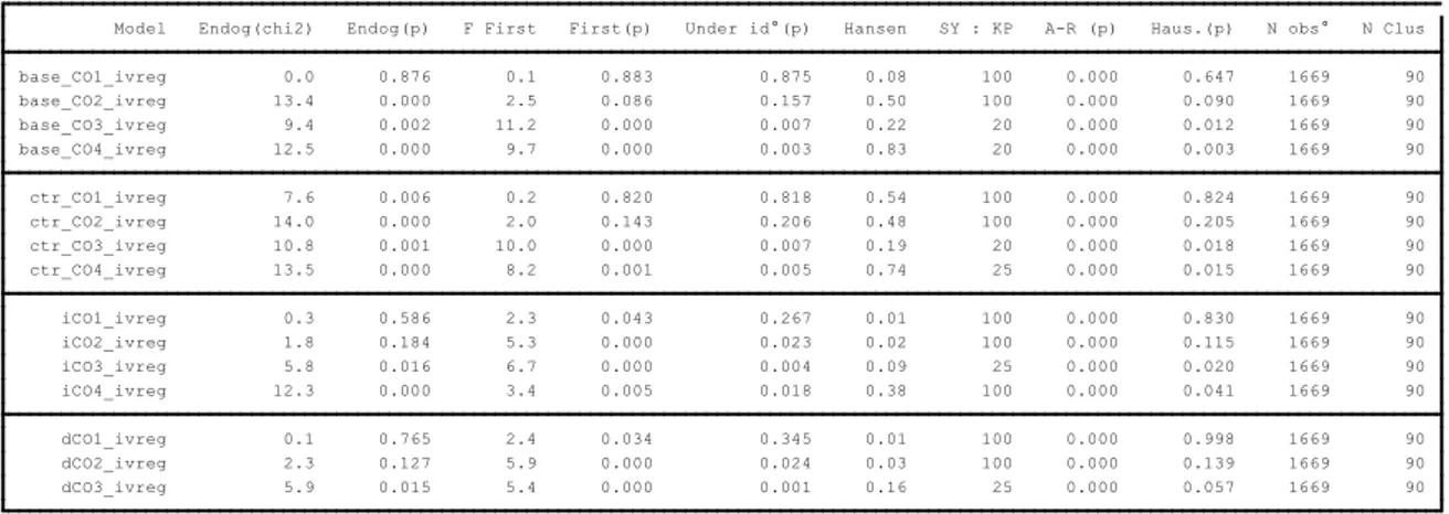
Assessment of the 2SLS models
In Table 6, the best specification is the base_CO3_ivreg model, meaning that the third level of severity is the best candidate to infer the effect of instrumented outages on connections. However, it entails only the outages variable, while the study aims to take account for the main potential omitted variable (poverty index) and its interaction with the outages. It would be thus better-off to switch to another equation, provided that the vector of tests will still hold.
Table 6 : ASSESSMENT OF THE 2SLS MODEL AT DISTRICTS LEVEL
dCO3_ivreg 5.9 0.015 5.4 0.000 0.001 0.16 25 0.000 0.057 1669 90 dCO2_ivreg 2.3 0.127 5.9 0.000 0.024 0.03 100 0.000 0.139 1669 90 dCO1_ivreg 0.1 0.765 2.4 0.034 0.345 0.01 100 0.000 0.998 1669 90 iCO4_ivreg 12.3 0.000 3.4 0.005 0.018 0.38 100 0.000 0.041 1669 90 iCO3_ivreg 5.8 0.016 6.7 0.000 0.004 0.09 25 0.000 0.020 1669 90 iCO2_ivreg 1.8 0.184 5.3 0.000 0.023 0.02 100 0.000 0.115 1669 90 iCO1_ivreg 0.3 0.586 2.3 0.043 0.267 0.01 100 0.000 0.830 1669 90 ctr_CO4_ivreg 13.5 0.000 8.2 0.001 0.005 0.74 25 0.000 0.015 1669 90 ctr_CO3_ivreg 10.8 0.001 10.0 0.000 0.007 0.19 20 0.000 0.018 1669 90 ctr_CO2_ivreg 14.0 0.000 2.0 0.143 0.206 0.48 100 0.000 0.205 1669 90 ctr_CO1_ivreg 7.6 0.006 0.2 0.820 0.818 0.54 100 0.000 0.824 1669 90 base_CO4_ivreg 12.5 0.000 9.7 0.000 0.003 0.83 20 0.000 0.003 1669 90 base_CO3_ivreg 9.4 0.002 11.2 0.000 0.007 0.22 20 0.000 0.012 1669 90 base_CO2_ivreg 13.4 0.000 2.5 0.086 0.157 0.50 100 0.000 0.090 1669 90 base_CO1_ivreg 0.0 0.876 0.1 0.883 0.875 0.08 100 0.000 0.647 1669 90 Model Endog(chi2) Endog(p) F First First(p) Under id°(p) Hansen SY : KP A-R (p) Haus.(p) N obs° N Clus
Introducing the poverty index (ctr_CO3_ivreg) yields the same Stock-Yogo threshold (20) as the base model (base_CO3_ivreg), with all the other tests being very close to the last.
Introducing further the interaction term (iCO3_ivreg) yields a weaker though acceptable Stock-Yogo threshold (25), with also the F of the first-stage being lower (6.7) since now there are two instrumented variables. Still, it’s above the targeted threshold (6), with a receivable p-value (0.000). The Anderson-Rubin test ensures that the model provides consistent estimates. All the second-order tests are also receivable.
Passing successfully all the tests, the iCO3_ivreg model appears to be robust enough: all the key factors, but the interaction, remain significant at 0.1% level (Table 7). As evidenced from its VIF (6.20), the lower significance of the interaction term is only due to the variance’s inflation once stepping from the OLS to the IV estimation.
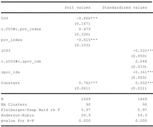
Table 7 : 2SLS OF CONNECTIONS AT DISTRICTS LEVEL (3 INSTRUMENTS)
In the districts where the rate of cumulative outages is higher, the household are less connected: where the frequency of outages is 1 percent point higher, the households’
connections level is -.806 percent point lower. From the standardized regression, the absolute magnitude of the outages’ impact on the connections’ level (-.231) is 43% higher than the one of the households’ poverty (-0.161).
Interacting both effects seems not significant, but the inflated test hides underlying differences in the significance level: while the Z-statistic behind Table 7 tests the distribution of the
* p<0.05, ** p<0.01, *** p<0.001 _________________________________________________________________ Seuils Stock-Yogo : 15.72, 9.48, 6.08, 4.7 c.WCP#c.pov_index c.fdr_moy_DISTRICT#c.pov_index c.fdr_vois_moy_DISTRICT#c.pov_index fdr_moy_DISTRICT fdr_vois_moy_DISTRICT WCP Excluded Instruments :
Instrumented variables : CO3 c.CO3#c.pov_index Variance : Robust robust cluster by DISTRICT IV (2SLS) estimation SE in parentheses. LHS : connection
pvalue for A-R 0.000 0.000 Anderson-Rubin 59.9 59.9 Kleibergen-Paap Wald rk F 5.97 5.97 Nb Clusters 90 90 N 1669 1669 (0.061) (0.031) Constant 0.762*** 0.502*** (0.020) zpov_idx -0.161*** (0.033) c.zCO3#c.zpov_idx 0.048 (0.050) zCO3 -0.231*** (0.103) pov_index -0.615*** (0.330) c.CO3#c.pov_index 0.479 (0.167) CO3 -0.806*** Unit values Standardized values
coefficient at average level of both terms, the significance of outages in this interaction may indeed be different given the poverty level (Graph 2)
Graph 2: MARGINAL EFFECT OF THE OUTAGES AT POVERTY LEVELS (2SLS)
The marginal effect is the derivative of the connections given the variation of outages: dc/do = -0.806 + 0.479. pov_index. It’s negative when pov_index < 0.806/0.479 = 1.68. Since pov_index ∈ [-1 ;1], the marginal effect of outages is always negative. However, as shown on Graph 3, it’s significant only when the poverty level is below 0.6: the outages have no
significant impact for the poorest households while they impact negatively the connection’s decision of the households with intermediate or higher wealth. The highest the wealth of the households, the more sensitive they are to the frequency of outages.
The linear specification was useful to identify the effect and the relevant severity level of its measurement, to bring the evidence of the impact using instrumental variables, and to get a first idea of the magnitude. However, the LPM does not ensured the predicted level to be a probability belonging to a [0;1] support. The shortcoming is all the more a constraint that the study aims to distinguish the connected from the unconnected households in a readable way, for eventual policy applications.
Non-linear modelling of the connection’s likelihood Probit estimation
For the outcome to be a probability, a Probit estimation is a more suitable method. Here, it’s designed to predict the likelihood of the connection, for the dependent variable equals 1 when an individual household is connected to the grid.
Assessment criteria
The criteria in Table 8 aim to diagnose the ability of the model to dissociate the connected and unconnected households, ie. to maximize the discriminatory accuracy of the model.
The first criterion is the lowest AIC. The second criterion is the lowest type I error (« T1 err. »), measuring the risk to predict a connection while the household is not connected. The third criterion is the highest specificity (« Id unconctd ») that measures the exact prediction of unconnected households, ie. the proportion of predicted unconnected households who are effectively unconnected. The forth criteria is the highest ROC : the area under the ROC curve is a synthetic measurement of the discriminatory accuracy of a probit/logit model. It does not depend on the cut-off, hence it gives an additional assessment, independent of the defined settings for a model’s application (see below). The fifth criteria is the smallest p-value of the outages. At this stage, the model should be enough discriminatory: one thus expect the
coefficient to be significant. If this test fails, one shall switch to the second-best specification. The sixth criteria is the lowest specification error of the unconnected (« C /- »), that is the proportion of truly connected households among the predicted unconnected households. It gives an expected approximation of the eventual operational cost of the model, since each of this error case would means an un-efficient cost of inquiry, prospection and commercial effort if the model were to be used on the field.
For a policy application, the model would indeed better off to minimize the prediction’s error of the unconnected households; therefore, the cutoff has been set to 75% in the diagnosis table (Table 8). As shown in Graph 3 such a level maximizes the return to specificity, ie. the ability to identify the unconnected households, at the cost of a lower recognition of the connected household (the sensitivity).9 However, one can reasonably expect that the benefit to decrease the marginal cost of the grid’s extension by increasing the proportion of recognized
unconnected households would be much higher than the usage’s cost of the model, measured by this specification error.
9 The sensitivity is the proportion of exact predictions of connections, ie. cases of predicted connected
Graph 3: TRADEOFF BETWEEN SPECIFICITY AND SENSITIVITY
Model iCO3_probit : power reliability index at third level of severity
Applying the aforementioned criteria, the best specification is achieved with iCO3 (Table 8). The Probit specification enhances the accuracy of the estimates (Table 9), compared to the OLS (Table 4): they are now all significant at 0.1% level.
Table 8 : ASSESSMENT OF THE PROBIT MODEL AT DISTRICTS LEVEL
0 .0 0 0 .2 5 0 .5 0 0 .7 5 1 .0 0 Se nsi tivi ty/ Sp eci fici ty 0.00 0.25 0.50 0.75 1.00 Probability cutoff Sensitivity Specificity dCO3 -1.378 0.427 0.001 1798 3.1 96.9 79.3 47.7 1669 90 dCO2 -1.133 0.254 0.000 1803 1.1 98.9 79.2 48.4 1669 90 dCO1 -1.136 0.319 0.000 1798 1.1 98.9 78.9 48.3 1669 90 iCO4 -0.960 0.429 0.025 1845 3.7 96.3 79.3 47.8 1669 90 iCO3 -1.108 0.231 0.000 1800 2.1 97.9 79.1 48.1 1669 90 iCO2 -1.091 0.250 0.000 1814 1.3 98.7 78.6 48.3 1669 90 iCO1 -1.252 0.371 0.001 1824 1.1 98.9 78.5 48.5 1669 90 ctr_CO4 -0.957 0.424 0.024 1844 2.0 98.0 79.3 47.8 1669 90 ctr_CO3 -0.821 0.215 0.000 1827 1.1 98.9 79.3 48.6 1669 90 ctr_CO2 -0.709 0.244 0.004 1843 1.3 98.7 79.0 48.5 1669 90 ctr_CO1 -0.243 0.315 0.440 1870 1.1 98.9 78.7 48.6 1669 90 base_CO4 -1.567 0.475 0.001 2194 6.2 93.8 65.4 56.7 1669 90 base_CO3 -1.375 0.206 0.000 2137 0.0 100.0 64.0 57.4 1669 90 base_CO2 -1.268 0.222 0.000 2179 0.0 100.0 59.1 57.4 1669 90 base_CO1 -1.088 0.286 0.000 2245 0.0 100.0 51.7 57.4 1669 90 Model Outages Std Error P value AIC T1 err. Id unconctd ROC C/- Nb obs° Nb Clus.
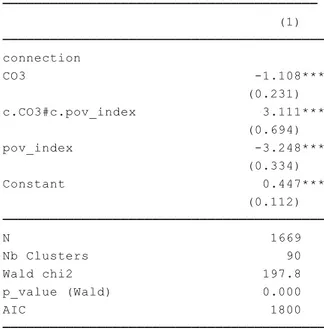
Table 9 : PROBIT OF THE CONNECTION AT DISTRICTS LEVEL
The Probit specification brings also a finest evaluation for the marginal effect of the interaction term (Graph 4)
Graph 4: INTERACTED MARGINAL EFFECTS (PROBIT)
As already identified with the linear specification, the poorest household are not sensitive to the quality of the distributed power (poverty index above 0.4, on the left). The highest sensitivity to outages is reached for households with a poverty index equals to -0.2. Conversely, there is a significant positive wealth effect in the districts where the outages remain under 80% (on the right). In the districts where the households are richer, the
likelihood to be connected is higher, provided that the reliability remains below an outages’ * p<0.05, ** p<0.01, *** p<0.001
_________________________________________ Variance : cluster by DISTRICT
Probit regression. SE in parentheses. LHS : connection AIC 1800 p_value (Wald) 0.000 Wald chi2 197.8 Nb Clusters 90 N 1669 (0.112) Constant 0.447*** (0.334) pov_index -3.248*** (0.694) c.CO3#c.pov_index 3.111*** (0.231) CO3 -1.108*** connection (1) -. 6 -. 4 -. 2 0 .2 Ef fe ct s on Pr(C on ne ct io n ) -1 -.9 -.8 -.7 -.6 -.5 -.4 -.3 -.2 -.1 0 .1 .2 .3 .4 .5 .6 .7 .8 .9 1 index_pauv
Marginal Effect of the Outages given the poverty level
-1 -. 5 0 .5 Ef fe ct s on Pr(C on ne ct io n ) 0 .1 .2 .3 .4 .5 .6 .7 .8 .9 1 (first) CO3
rate of 80%. On the opposite, a too extremely low reliability of the power vanished the positive wealth effect of the households.
IV Probit estimation
Though the Probit yields more consistent estimates for a probability outcome, it might be poised by the risks of endogeneity. It is now necessary to instrument the outages the same way as in the linear specification. Stata provides a dedicated procedure -ivprobit- that combines the Probit modeling of a likelihood and linear regressions to instrument the endogenous variables. Unfortunately, the available tests to assess the instrumentation’s quality are not as much developed as they are in the -ivreg2- procedure, because, as recalled by Wooldridge, the diagnosis shall be made in a linear setting.10
Therefore, the assessment of the instrumentation’s quality made above remains, leading to keep the chosen specification iCO3. For the sake of consistency, the assessment table (Annex 7) exhibits the key available tests of instrumentation in –ivprobit-, to check whether the model still holds while upgrading the method. The AIC and the ROC are also verified, to ensure that the discriminatory capacity of the model still holds.
The diagnosis criteria (Annex 7) are read in the following order: - Endogeneity Wald test below 1% ;
- Forced Hausman test below 5% ;
- Global Wald test of the specification below 1% ;
- Z-test of the estimates of the first instrument in the first-stage below 1% ; - ROC among the highest values ;
- AIC among the smallest values.
The iCO3_ivprobit specification meets all these ordered criteria but the AIC (1451). Its ROC is the best (77%), proving that this specification remains solid with respect to its
discriminatory ability (Annex 7). However, going backward along the chain of tests, the p-value of the lightning is significant at only 9% level, what is not enough for the main instrument to achieve its purpose. Switching to the lowest AIC (-301 for iCO1) would provide inconsistent instrumentation with respect to the endogeneity test (0.314), the p-value of lightning (0.666) and the Hausman test (1.000). Switching to the next best AIC (587 for iCO4) would also yield a poor instrumentation (Hausman : 8.5% and p-value of lightning :
10 http://www.statalist.org/forums/forum/general-stata-discussion/general/1295919-underidentification-and-weak-identification-test-for-ivprobit
0.854). The risk that the estimates of the instrument would be biased is too high for any specification, yielding a too high risk that the endogenous issues would not be properly tackled in the reduced form.
Looking at the first-stage, Annex 8 indicates that the issue arises from the lightning by neighbor. Though there is no advanced test of over-identification in the IVPROBIT procedure, it looks intuitive that too many linear components in the first-stage regression might actually over-fit the model for a non-linear estimation. One thus keep only the two mainly significant instruments in the iCO3 specification: the lightning (fdr_moy_DISTRICT : 0.090) and the weighted distance to the closest electrical plant (WCP : 0.000).
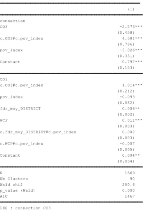
Reading again the decision criteria (Annex 9), the iCO3 specification with two instruments appears now to pass successfully all the tests, still showing the best discriminatory ability (ROC : 76.8) while the instrumentation becomes much more consistent (Endogeneity : 0.000, p-value of the lightning in first-stage : 0.006, Hausman : 0.017). The model iCO3_ivprobit exhibits accurate estimates at 0.1% level for all the variables in the reduced form (Table 10), with only the excluded instruments being strongly significant in the first-stage (below 1%). Yielding both accurate and unbiased estimates of the outages’ impact on the households’ connection, it’s renamed “scoring grid” and retained as the preferred specification.
Table 10: CONNECTION’S SCORING GRID
It could be applied to infer the likelihood that any new household out-the-sample would not be connected, provided that the same data could be gathered to feed the scoring grid.
* p<0.05, ** p<0.01, *** p<0.001
________________________________________________________
At district level with 2 instruments (lightning, weighted closest plant) Variance : cluster by DISTRICT
Probit model with endogenous regressors SE in parentheses. LHS : connection CO3 AIC 1467 p_value (Wald) 0.000 Wald chi2 250.6 Nb Clusters 90 N 1669 (0.034) Constant 0.094** (0.005) c.WCP#c.pov_index -0.007 (0.003) c.fdr_moy_DISTRICT#c.pov_index 0.002 (0.003) WCP 0.011*** (0.002) fdr_moy_DISTRICT 0.006** (0.062) pov_index -0.093 (0.212) c.CO3#c.pov_index 1.014*** CO3 (0.153) Constant 0.797*** (0.331) pov_index -3.026*** (0.786) c.CO3#c.pov_index 4.581*** (0.458) CO3 -2.573*** connection (1)
Impact evaluation of the outages on the connection’s decision in a context of poverty
As the model now consistently neutralizes the three risks of endogeneity, it can be confidently used to explore and compare the effects of reliability and poverty. Relying on (Williams, 2012), the study explores the predictions and marginal effects, whether with the observed values of the sample or at different referral levels of the outages and poverty.
Annex 14 checks the initial statistical conditions of this evaluation.
The predicted probability to be connected is not linear, neither in the outages nor in the poverty level (Graph 5). Interestingly, the predicted connection’s probability is not complete given the outages: while the probability to find any connected household is almost 0 when the rate of partial severity outages reaches 100% in a district, it’s up to 80% when the rate of the same severity’s outages is 0. There might be additional occasional outages (4-level severity) that could possibly have a residual effect, deterring the households to subscribe to the grid. This point will be addressed with the “extension“ model (section VII).
Graph 5 : DIRECT EFFECT OF OUTAGES AND POVERTY ON CONNECTION’S PROBABILITY (APM)
One will now explore how the prediction’s change from a referral level, when outages or poverty deviate from their mean or any other referral values in the sample. Graphically, it’s equivalent to assess the slopes of the above prediction at different points (eg. CO3), fixing the other predictor (eg. pov_index) at a specific level (its mean or eventually its median). The marginal effects in Table 11 will all be assessed in absolute value, using eventually the standardized regression for any comparison (table 11, 2nd span).
0 .2 .4 .6 .8 1 Pro ba bi lit y O f Po si tive O ut co me 0 .1 .2 .3 .4 .5 .6 .7 .8 .9 1 (first) CO3
Adjusted Predictions with 95% CIs
0 .2 .4 .6 .8 1 Pro ba bi lit y O f Po si tive O ut co me -1 -.9 -.8 -.7 -.6 -.5 -.4 -.3 -.2 -.1 0 .1 .2 .3 .4 .5 .6 .7 .8 .9 1 index_pauv
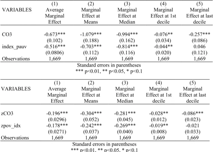
Table 11 : MARGINAL EFFECTS OF OUTAGES AND POVERTY
On average, 1 percent point more outages causes 0.673 percent point less connected households. At the average values in sample, 1 percent point more outages causes 1.079 percent point less connected households or 0.994 less in a median district.
Once standardized, the Average Marginal Effect of outages (-0.196) is 10% higher than the solely effect of poverty (-0.178). However, this estimates depends on the fit of outages’ and poverty’s distributions in the sample to their true distributions in the Kenyan population, hence of the representativeness of the sample. Without any previous adequacy tests (eg. : Kolmogoroff-Smirnoff), the trueness of this estimation is hard to assess. Nonetheless, with 1,669 observations, a normal distribution can be confidently assumed for the poverty index, and so it is in the sample (not shown). Applying the central-limit theorem, its means can be considered as a referral value, already converging to and thus representative of its true value in the population. But outages are not normally distributed over the sample (not shown). It’s thus necessary to compare the marginal effects at several referral values of the index.
Comparing districts at average levels of outages and households’ poverty (Table 11, column 2), the impact of outages (-0.304) is 26% higher than the one of poverty (-0.242). This result
(1) (2) (3) (4) (5) VARIABLES Average Marginal Effect Marginal Effect at Means Marginal Effect at Median Marginal Effect at 1st decile Marginal Effect at last decile CO3 -0.673*** -1.079*** -0.994*** -0.076** -0.257*** (0.102) (0.188) (0.162) (0.034) (0.086) index_pauv -0.516*** -0.703*** -0.814*** -0.044** 0.046 (0.0806) (0.112) (0.116) (0.020) (0.121) Observations 1,669 1,669 1,669 1,669 1,669
Standard errors in parentheses *** p<0.01, ** p<0.05, * p<0.1 (1) (2) (3) (4) (5) VARIABLES Average Marginal Effect Marginal Effect at Means Marginal Effect at Median Marginal Effect at 1st decile Marginal Effect at last decile zCO3 -0.196*** -0.304*** -0.281*** -0.028** -0.086*** (0.0296) (0.052) (0.045) (0.012) (0.023) zpov_idx -0.178*** -0.242*** -0.269*** -0.019** -0.021 (0.0271) (0.037) (0.040) (0.008) (0.033) Observations 1,669 1,669 1,669 1,669 1,669
Standard errors in parentheses *** p<0.01, ** p<0.05, * p<0.1
brings the evidence that the main obstacle to increase subscriptions to the electricity is much more the power reliability than the household’s poverty.
Comparing two median districts would be more robust (Table 11, column 3). In that case, the impact of outages (-0.281) still remains 5% higher than the one of poverty (-0.269), a result to keep as a lower bound.
For two representative districts in the best situation, being respectively in the first decile of the reliability and in the first decile of the poverty index (Table 11, column 4), the impact of outages (-0.028) is 47% higher than the one of poverty (-0.019).
Being now in the worst districts from the last decile, with the highest outages rate and the highest poverty index (Table 11, column 5), the poverty has no more significant impact on the connection’s decision. In those districts, the households are only sensitive to the outages (-0.086), but three times less than in the median districts (-0.281).
Beyond the global evaluation, the impact of outages and poverty are not always the same with respect to their own level (Graph 6) or taking into account their interacted effect (Graph 7).
Graph 6 : CONDITIONAL EFFECTS OF OUTAGES AND POVERTY ON THE CONNECTION’S PROBABILITY (MEM)
The marginal effect of outages is of maximum magnitude (in absolute value) in the districts where the rate of partial severity outages reaches 30% (Graph 6, left : -1.09). There, any quality upgrade of the distributed power might have the maximum potential to trigger new subscriptions. On the opposite, in the districts were the partial severity’s outages are very frequent (100%), their impact is lower (-0.203), while still significant: there, any reliability upgrade might only have a smooth effect on connections. Since the frequency of outages might be perceived as far too high, the households might be reluctant to believe in any reliability’s enhancement. The channel might also surge through the interaction with the poverty level in this kind of districts, as it will be discussed afterward.
-1 .5 -1 -. 5 0 Ef fe ct s on Pro ba bi lit y O f Po si tive O ut co me 0 .1 .2 .3 .4 .5 .6 .7 .8 .9 1 (first) CO3
Conditional Marginal Effects of CO3 with 95% CIs
-1 -. 8 -. 6 -. 4 -. 2 0 Ef fe ct s on Pro ba bi lit y O f Po si tive O ut co me -1 -.9 -.8 -.7 -.6 -.5 -.4 -.3 -.2 -.1 0 .1 .2 .3 .4 .5 .6 .7 .8 .9 1 index_pauv
The model also captures the role of intermediate wealth (Graph 6, right): the magnitude of the marginal effect is maximum (-0.71) when the poverty index reaches 0, a central level of the index. Among the households with intermediate wealth, being one unit richer (decreasing index, toward the left) has the maximal potential effect to observe more subscriptions. On the opposite, among the richest households (pov_index = -1), the wealth effect is much less sensitive (-0.172): for them, any lower level in wealth (increasing poverty index, toward the right) has only a smooth negative marginal effect on the connection’s decision. It’s also the case among the poorest households (-0.120): for them, being one unit better-off (decreasing poverty index, toward the left) leads to observe only a slightly higher level of connections. The underlying reason of this non-linear wealth effect might also be due to its interaction with the outages intensity.
Graph 7 : INTERACTED EFFECTS OF OUTAGES AND POVERTY ON THE CONNECTION’S PROBABILITY (MEM)
Not only the reliability’s impact is not the same way significant according to the level of poverty, but in addition, its magnitude is not linear given the poverty level (Graph 7, left). For a poverty index between 0.4 and 0.7, the outages have no significant impact on the
connection’s decisions. Above 0.8, the impact is borderline significant and might be
considered cautiously. Bellow -0.9, the outages are neither significant, and since the width of the confidence interval is growing while the index is decreasing, the -0.8 level should also be considered cautiously.
Finally, the outages have a negative significant marginal effect among the households with a poverty index between -0.7 and 0.3, but not substantively of the same intensity: in absolute value, its magnitude is maximum (-1.28) for a poverty index equal to -0.3. The low reliability has the maximum deterring impact among the households with intermediate wealth: in other words, those are the most reluctant to subscribe in presence of outages. Said in positive terms,
-2 -1 .5 -1 -. 5 0 .5 Ef fe ct s on Pro ba bi lit y O f Po si tive O ut co me -1 -.9 -.8 -.7 -.6 -.5 -.4 -.3 -.2 -.1 0 .1 .2 .3 .4 .5 .6 .7 .8 .9 1 index_pauv
Conditional Marginal Effects of CO3 with 95% CIs
-1 -. 5 0 .5 Ef fe ct s on Pro ba bi lit y O f Po si tive O ut co me 0 .1 .2 .3 .4 .5 .6 .7 .8 .9 1 (first) CO3
for any higher reliability, the intermediate wealthy households would be the most prone to subscribe.
Conversely, in the districts where the rate of partial severity’s outages is too high (above 50%), the poverty index is not significant (Graph 7, right). In the districts too much exposed to outages, the wealth or poverty of the households is not the reason why they do not
subscribe. On the opposite, in the districts benefiting a higher reliability (outages’ rate below 40%) the wealth level contributes to explain the household’s decision to subscribe but with a maximum magnitude (-0.837) that is 35% lower than their sensitivity to outages (-1.28). To sum up : the wealth effects exists only in the districts exposed to a low level of outages, while the low reliability deters at most the unconnected intermediate wealthy households to subscribe. Those last would be the most prone to subscribe for any improvement of the reliability, provided that they’re living in a district were the outages are not already too frequent among their neighbors.
VI - Robustness checks
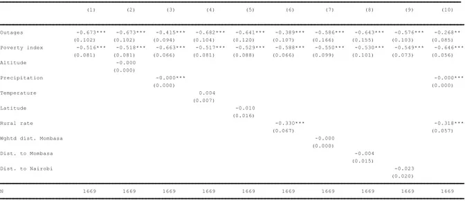
Table 12 controls for the stability of the outages’ estimate in the preferred specification (column 1), with respect to potentially omitted variables.
Columns 2 to 5 follow (Andersen and Dalgaard, 2013), with altitude replacing the coastal dummy. As they found, the outages’ effect is robust to the inclusion of Altitude, Temperature and Latitude : introduced one at a time, they’re not significant and modify only slightly the marginal effect of outages.
The precipitations (column 3) seems to be significantly correlated with a lower level of connections in Kenya. They do not change the direction of the outages’ impact, but this omitted variable reduces substantially their magnitude (-0.415), while (Andersen and Dalgaard, 2013) had found them to be insignificant.
Most likely, rainfalls could be partially correlated with the storms, capturing a partial effect of lightning and thus also of the outages. Actually, the western provinces are much more
exposed both to rainfalls and lightning than the arid north-eastern regions (Map 1). There is a specific heterogeneity of precipitations in Kenya correlated with lower connections, that was not in the country-level data of (Andersen and Dalgaard, 2013). However, as evidenced from its VIF in the 2SLS settings (1.01), precipitations are fully orthogonal to the hyperplan of the other variables, meaning that their inclusion could well capture the direct area effect on individual connections, as diagnosed in the qualitative causal assessment (Annex 4).
Table 12 : ROBUSTNESS TO ADDITIONAL CONTROLS
The rural location (Table 12, column 6) is also correlated with a lower connections’ level (-0.330), yielding a lower though still negative estimate for outages (-0.389). In 2014,
connections to the electrical grid are less likely to be observed in rural districts of Kenya. In a policy perspective, this stake is directly addressed by the REA.
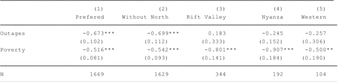
Taking into account both variables together (Table 12, column 10) reduces the marginal effect of outages (-0.268) while still keeping its negative sign. In western rainy Provinces, Kenya has developed a specialization in sugar cane and tea plantations, managed by multinational firms, or Kenyan farms supported by the Kenyan Tea Development Agency (KTDA). In both cases, the transformation requires electricity. But due to the unreliability of the power, the firms produce it from their own installations, with bio-generation or small hydro power generators, selling the remaining excess to the grid, if any. The correlation of the rainfall and rural location with lower connections could simply reflect this peculiar economy in lower connected districts (see Map 2 and Annex 12).
The results of (Khandker et al., 2014) also suggested a possible arbitrage between an electrical connection and the price of kerosene. This last is approximated by the distance to Mombasa weighted by the difficulty of the road (Table 12, column 7), but is neither
significant nor it has the expected sign. Turning to absolute distance to the main activity centers in Mombasa and Nairobi (column 8 and 9) is neither significant.
As seen in section IV and also suggested by the results of (Lee et al., 2014), it’s needed to check for any residual correlation of the shelter’s type with the error term (Annex 10). The
* p<0.05, ** p<0.01, *** p<0.001
____________________________________________________________________________________________________________________________________________ Variance : Robust cluster
(lightning, weighted closest plant) ivprobit at district level with 2 instruments Average marginal effects SE in parentheses. Probability of positive outcome (connection)
N 1669 1669 1669 1669 1669 1669 1669 1669 1669 1669 (0.020) Dist. to Nairobi -0.023 (0.015) Dist. to Mombasa -0.004 (0.000) Wghtd dist. Mombasa -0.000 (0.067) (0.057) Rural rate -0.330*** -0.318*** (0.016) Latitude -0.010 (0.007) Temperature 0.004 (0.000) (0.000) Precipitation -0.000*** -0.000*** (0.000) Altitude -0.000 (0.081) (0.081) (0.066) (0.081) (0.088) (0.066) (0.099) (0.101) (0.073) (0.056) Poverty index -0.516*** -0.518*** -0.663*** -0.517*** -0.529*** -0.588*** -0.550*** -0.530*** -0.549*** -0.646*** (0.102) (0.102) (0.094) (0.104) (0.120) (0.107) (0.166) (0.155) (0.103) (0.085) Outages -0.673*** -0.673*** -0.415*** -0.682*** -0.641*** -0.389*** -0.586*** -0.643*** -0.576*** -0.268** (1) (2) (3) (4) (5) (6) (7) (8) (9) (10)