Non-Mercer Kernels for SVM Object Recognition
Sabri Boughorbel
1Jean-Philippe Tarel
2Franc¸ois Fleuret
3[email protected]
[email protected]
[email protected]
1,3
IMEDIA Research Group
2Division of ESE
BP 105
LCPC
INRIA Rocquencourt
35 Boulevard Lefebvre
78150 Le Chesnay, France
75732 Paris Cedex 15, France
Abstract
On the one hand, Support Vector Machines have met with significant success in solv-ing difficult pattern recognition problems with global features representation. On the other hand, local features in images have shown to be suitable representations for effi-cient object recognition. Therefore, it is natural to try to combine SVM approach with local features representation to gain advantages on both sides. We study in this paper the Mercer property of matching kernels which mimic classical matching algorithms used in techniques based on points of interest. We introduce a new statistical approach of ker-nel positiveness. We show that despite the absence of an analytical proof of the Mercer property, we can provide bounds on the probability that the Gram matrix is actually pos-itive definite for kernels in large class of functions, under reasonable assumptions. A few experiments validate those on object recognition tasks.
1
Introduction
Objects recognition in variable contexts under different illuminations remains one of the most challenging problem in computer vision and artificial intelligence. Compared to the efficiency of human brain, algorithms have been unable so far to demonstrate competitive performances in real usage conditions.
Among all the techniques developed during the last decades, points of interest in com-puter vision [17, 16, 10] and support vector machines (SVMs) in statistical learning [5, 1] have been successful in solving many real-world problems.
Points of interest based techniques combine the information provided by the responses of local filters at several highly informative locations in the picture and their global ge-ometric configuration. Such approaches lead to compact and invariant representations. SVM algorithms search the optimal separating plane between positive and negative ex-amples. It has the advantage of high generalization capacity from a few training exex-amples. In some sense, points of interest techniques and SVMs address two different issues. While the formers provide a very meaningful way to represent and compare images, the laters are able to combine several training examples into a consistent and statistically sound view-based representation.
A few attempts have tried recently to combine those two approaches into a common framework by building kernels on the space of feature vector sets [4, 19, 21, 12]. While kernels are usually defined on vector spaces, they have to deal in this new context with features of various size where no order is defined between components. Also, since the classical matching algorithm used in points of interest techniques are able to tackle the occluding problem and to provide invariance to the pose, it seems highly desirable that the used kernels mimic those matching algorithms.
The SVM problem is convex whenever the used kernel is a Mercer one. The convexity insures the convergence of the SVM algorithm towards a unique optimum. The unique-ness of the solution is one of the main advantages of the SVM compared to other learning approaches such as neural networks. Unfortunately, as we will see, numerous examples show that using matching algorithms as kernels for SVM are not in general Mercer.
Nevertheless the use of simple matching algorithms as kernels gives good results in practice. This experimental observation leads us to consider the positiveness of the kernel from a statistical point of view. We show that, even if kernels based on matching are not always positive, this is likely to be true for a large class of functions. Moreover, we propose a way to control the probability of positiveness by tuning kernel parameters in this class. This control can be also used with advantages in many other applications where SVM approach applies, with local and global representations as well.
In §2 we present different approaches for recognition with local features, in §3 we present our main result of bound on the Gram matrix probability to be positive definite and give experimental results in §4.
2
Recognition With Local Features
Let X be the space where the features are taken from (Rnfor example). The dimension of X is in general finite and fixed. In the context of recognition from images, this implies that the used representation is global on the image. Therefore, in such a case, the design of a kernel for object recognition is closely related to template matching. This family of algorithms is mainly based on correlations between two images. In [3], Mercer kernels for object recognition in images are build based on such template matching algorithms. Two main drawbacks of template matching algorithms are known to be their computational cost and poorly robust results in case of occlusion.
2.1
Local Feature Representations
To better tackle these difficulties, local features representation were introduced for im-ages. The idea is, first to build a detector of particular points in images, usually called
points of interest (or key points, anchors points, salient points), and second to
character-ize each point by its local environment. This obtained set of features is the local feature representation of an image. This kind of representations have shown to be suitable rep-resentations of images for object recognition, see for instance [17, 10]. Indeed, the infor-mation about images has been drastically reduced, allowing faster comparison algorithms than using correlation based algorithms. There is many ways to locally characterize the environment of a point. The most used feature seems to be the so-called jet, which is the vector based on a differential characteristic’s around the point of interest. However, following [16], SIFT feature seems to provide improvement to jet features.
2.2
Point Matching Algorithms
Given two images of the same object, each image being represented by a set of local fea-tures X and X0, occlusion may remove several points of interest in one or in the other image. Moreover, due to complex background, extra points appear as outliers. There-fore, correspondences must be robustly established between the two sets X and X0. This task can be performed by matching algorithms. Depending on the constrains enforced on matching (bijective, symmetric,...), different algorithms were derived (see [22] for a partial review). Optimal matching algorithms have to face with combinatorial explosion, and thus many matching algorithms are in practice based on heuristics.
The result of the matching algorithm is two index functions Φ1(n) ∈ [1, ..., NX] and
Φ2(n) ∈ [1, ..., NX0] that gives the indices of the N matched pairs of feature vectors
(xΦ1(n), yΦ2(n))1≤n≤N, where NX and NX0 denotes the size of sets X and X
0
3
Kernels for Sets
Recent works [13, 9, 12, 21] have focused on designing Mercer kernels for different kinds of structured features such as strings, DNA, graphs, trees, and sets.
Any Mercer kernel can be written as an inner product after mapping by a well-chosen
f function [5], i.e K(x, x0) = hf (x), f (x0)i. Thus, Mercer kernels can be seen as a
measure of dissimilarity between vectors x and x0.
3.1
Known Kernels
For local feature representations, the simplest approach is to define the global dissimilarity between two sets of vectors as the sum over dissimilarities between all possible pairs of vectors. The dissimilarity of a pair of vectors is obtained by a Mercer kernel k(xi, x0j).
The Summation Kernel is thus:
KS(X , X0) = NX X i=1 NXX 0 j=1 k(xi, x0j) (1)
We may use RBF kernel for k:
k(xi, x0j) = e− kxi−x0j k2
2σ2
where σ is the scale parameter. Although the numbers NX and NX0 of vectors in the two
sets X and X0are not fixed, it can be proved that KS is a Mercer kernel [11]. However,
the number of pairs is increasing more rapidly than the number of vectors. Thus using KS, correct correspondences are swamped into bad correspondences.
In [21] a Mercer kernel is proposed for sets of vectors based on the concept of principal angles between two linear subspaces. This last approach is interesting but the proposed kernel is invariant when local feature vectors xiare combined linearly. Thus, this kernel
does not match our practical needs. In [12], another approach is proposed where the set is represented as a mixture of gaussian. This approach requires relatively dense sets of vectors to be meaningful, which is difficult to achieve in practice.
3.2
Matching Kernel
A better approach to compute global dissimilarity between two sets of local feature vec-tors extracted from two images is to take into account only dissimilarities between matched local features. Thus, the global dissimilarity is defined by:
KM(X , X0) = N X n=1 k(xΦ1(n), x 0 Φ2(n)) (2)
where Φ1(n) ∈ {1, ..., NX}, Φ2(n) ∈ {1, ..., NX0} denote the mappings between the two
sets of vectors, like in Sec. 2.2. N denotes the number of matched pairs of vectors, and thus we have N ≤ min(NX, NX0).
The optimal mapping (Φ∗1, Φ∗2) is obtained as the one that maximizes the dissimilarity, so:
(Φ∗
1, Φ∗2) = arg maxΦ
1,Φ2
KM(X , X0) (3)
Since the exact solution of the previous problem is time consuming, as explained in Sec. 2.2, we better use an heuristic as matching algorithm. We have used the
winner-take-all approach: at each step, the pair of points having the maximum dissimilarity is
matched and the associated vectors are removed to future examinations for the next steps. We notice that in general the mapping depends on sets X and X0, and thus, contrary to [19], it is not easy to prove that KM(X , X0) is a Mercer kernel, even when the local
kernel k is Mercer. If the assertion “the max of Mercer kernels is still a Mercer kernel” was true, we could prove that KM(X , X0) is Mercer. Unfortunately, the max of Mercer
kernels is not Mercer [2], and even not conditionally positive definite [18].
A simple counter example is now presented. We consider the matrices G1, G2 and
G3= max(G1, G2), with eigenvalues λirespectively, as: G1= 2 6 6 4 2 −1 −2 −1 2 3 −2 3 8 3 7 7 5 λ1= 2 6 6 4 0.72 1.4 9.8 3 7 7 5 G2= 2 6 6 4 7 4 −2 4 3 −1 −2 −1 1 3 7 7 5 λ2= 2 6 6 4 0.29 0.68 10.02 3 7 7 5 G3= 2 6 6 4 7 4 −2 4 3 3 −2 3 8 3 7 7 5 λ3= 2 6 6 4 −0.92 9.34 9.57 3 7 7 5
G1 and G2 are two positive definite Gram matrices but their max (G3) is not. This
suggests that in general matching algorithms are not Mercer kernels. Indeed, we have found other more complicated counter-examples to Mercer or conditional positiveness, for optimal matching algorithm.
3.3
Statistical positiveness of Kernels
In [19, 2, 6] non-Mercer kernels have been used for SVM based pattern recognition. Although performances of these kernels are good, the convergence of SVM algorithm to the unique optimum is not insured since there is no warranty that the SVM optimization
problem is convex. We introduce next a new definition of kernel positiveness based on a statistical approach. This definition is general enough to include usual Mercer kernels. The advantage is that we can show that matching kernels are statistically positive definite kernels.
We denote here by X1, . . . , X` a family of ` i.i.d random variables standing for the
training samples. We want to bound the probability that the Gram matrix (Kσ(Xi, Xj))i,j
violates the Mercer condition, σ is the tuning scale hyperparameter of the kernel. A suffi-cient condition for the Gram matrix to be positive definite is to be diagonal dominant. We recall, that a matrix G is called diagonal dominant when for each i, we have:
|Gii| ≥
X
i6=j
|Gij| (4)
Diagonal dominance condition is an easy way to enforce Mercer condition directly on the Gram matrix. It has been used besides to derive kernels for strings [20]. In the following, McDiarmid concentration inequality [15] is recalled and a modified version is introduced. Many concentration inequalities can be found in the literature [14] like Hoeffding, Bennett ones, but they are useless in our case because of too strict assumptions with respect to independence. McDiarmid inequality will allow us to rewrite diagonal dominance condition in a statistical point of view.
Theorem. McDiarmid inequality (1989)
X1, . . . , X`be independent random variables ∈ A.
Let f : (A)`→R satisfies the bounding difference property: sup x1,...,x` x0i∈A ∈A|f (x1, . . . , x`) − f (x1, . . . , xi−1, x 0 i, xi+1, . . . , x`)| ≤ ci, 1 ≤ i ≤ `
Thus, the following probability is bounded by:
∀² > 0, P {f (X1, . . . , X`) − E (f (X1, . . . , X`)) > ²} ≤ e − 2²2
P`
i=1 c2i
In the case of 0 ≤ f (x1, . . . , x`) < m, where m ¿ ciwith a high probability but not
equal to 1, McDiarmid inequality leads to a poor bound. To solve the problem, we give next an improvement of the McDiarmid inequality in the case of positive function f .
Lemma. Modified McDiarmid inequality
Let M > 0 such that P (0 ≤ f (X1, . . . , X`) ≤ M ) = 1,
for 0 < η < 1, let 0 < m < M such that P (0 ≤ f (X1, . . . , X`) < m) = η then
∀² > 0, P {f (X1, . . . , X`) − E (f (X1, . . . , X`)) > ²} ≤ ηe− 2²2 `m2 + (1 − η)e− 2²2 `(M −m)2 Proof. 1{0≤f (x1,...,x`)≤M }=1{0≤f (x1,...,x`)<m}+1{m≤f (x1,...,x`)≤M }
the two events are disjoint and we have : P©1{f (X1,...,X`)<m} ª = η |f (x1, . . . , x`) − f (x01, . . . , x0`}| < m since 0 ≤ f (x1, . . . , x`) < m P¡1{m≤f (X1,...,X`)≤M } ¢ = 1 − η |f (x1, . . . , x`) − f (x01, . . . , x0`)| ≤ M − m since m ≤ f (x1, . . . , x`) ≤ M
We obtain the modified McDiarmid inequality by applying McDiarmid inequality on the two terms on the right:
P {f (X1,...,X`)−E(f (X1,...,X`))>²} = η P {f (X1,...,X`)−E(f (X1,...,X`))>²}+
+(1−η) P {f (X1,...,X`)−E(f (X1,...,X`))>²}
≤ ηe−`m22²2 + (1 − η)e−
2²2
`(M −m)2
Some assumptions are given on the kernel, we suppose that the kernel is constant on the diagonal, i.e. Kσ(xi, xi) = k, a wide class of kernel verifies this assumption,
for example kernels like Kσ(x, y) = g(kx−ykσ ) . In our case the matching kernel also
belongs to this class. Another assumption is that the kernel is positive and bounded, i.e.
0 ≤ Kσ(x, y) ≤ c for x, y ∈ X. Last assumption is on the asymptotic behavior of the
kernel with respect to the parameter σ, Kσ(x, y) −→
σ→0 0 for x 6= y which mean that the
kernel vanishes at infinity.
Proposition. Let Kσbe a kernel, with a hyperparameter σ, satisfying the following
con-ditions: Kσ(x, x) = k, 0 ≤ Kσ(x, y) ≤ c and Kσ(x, y) −→ σ→00.
Let pdbe the probability that the Gram matrix of the kernel Kσnot being diagonal
dom-inant. Xiwith i = 1, . . . , ` are ` i.i.d random variables representing training samples:
pd= P ∃i0, ` X j=1 j6=i0 Kσ(Xi0, Xj) > Kσ(Xi0, Xi0) for 0 < η < 1, there exists σ such that we bound pdas following:
pd≤ ` µ η exp ½ −2(k − (` − 1)eσ)2 (` − 1)m2 σ ¾ + (1 − η) exp ½ −2(k − (` − 1)eσ)2 (` − 1)(M − mσ)2 ¾¶ (5)
where eσ= E (Kσ(X1, X2)), M = (` − 1)c and mσis defined by
P (f (X1, . . . , Xn) < mσ) = η
Proof. We define the function fias the following
fi(x1, . . . , x`) = ` X j=1 j6=i Kσ(xi, xj)
since Kσ is bounded, we have 0 ≤ fi(x1, . . . , x`) ≤ M, where M = (` − 1)c. As a
consequence, fi satisfies the bounding property of modified McDiarmid inequality. The
there exists a line from the Gram matrix that does not satisfy dominance condition (4). pd = P {∃i0,P`j=1 j6=i0 Kσ(Xi0, Xj) > Kσ(Xi0, Xi0)} = P {∃i0,P`j=1 j6=i0 Kσ(Xi0, Xj) > k} ≤ P` n=1P {P`j=1 j6=n
Kσ(Xn, Xj) > k} since union bound propriety
= ` P {P` j=1 j6=i
Kσ(Xi, Xj) > k} since Xjare i.i.d
= `P {fi(X1,...,X`)>k}
= `P {fi(X1,...,X`)−E(fi(X1,...,X`))>k−E(fi(X1,...,X`))}
= `P {fi(X1,...,X`)−E(fi(X1,...,X`))>k−(`−1) E(Kσ(X1,X2))
| {z }
eσ }
= `P {fi(X1,...,X`)−E(fi(X1,...,X`))>²σ} (6)
where ²σ= k − (` − 1)eσ. We need to insure ²σ> 0 to apply McDiarmid inequality. We
have by definition eσ = E(Kσ(X1, X2) =
R
Kσ(x, y)dP (x, y). As we supposed that
Kσ(x, y) −→
σ→00, we deduce eσ−→σ→00 and thus there exists a σ such that ²σ> 0.
We consider the following interval subdivision :
1{0≤fi(x1,...,x`)≤M }=1{0≤fi(x1,...,x`)≤mσ}+1{mσ<fi(x1,...,x`)≤M }
For this subdivision, we now apply the modified McDiarmid inequality on equation (6) and we thus deduce (5).
The confidence term η can be chosen close to one to insure that second term of the bound (5) is very small.
For a given η, we choose mσ> 0 such that η = P {fi(X1, . . . , Xn) < mσ}.
We choose σ as small as needed to insure the first term of (5) to be small enough. This is always possible. Indeed, Markov inequalities implies that
1 − η = P {fi(X1, . . . , Xn) > mσ} ≤ (` − 1)mσeσ , so we obtain that mσ≤ (` − 1)1−ηeσ .
As shown previously, eσ −→
σ→0 0, thus mσ σ→0−→ 0, therefore the first term of (5) goes to
0. As a consequence, it is possible to enforce kernel positiveness with high probability by tuning kernel hyperparameters. If the obtained Gram matrix has a too large diagonal, generalization performance of the SVM classifier can be poor, but we can use a technique presented in [8, 7] that solve such problem.
It is known that the L2-SVM soft margin is equivalent to adding a ridge to the Gram
matrix [5]. Thus such regularization forces the Gram-matrix towards diagonal dominant ones.
4
Results
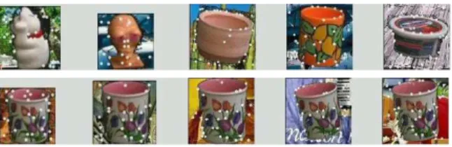
The database used in our experiments (see Fig. 4) contains about 165 images of 128× 128 pixels obtained by encrusting complex background images to original images of the same object which are taken from COIL-100 Database to generate positive samples. Similarly, negative samples are obtained by a random choice of objects images of the COIL-100 Database.
Points of interest are extracted with Harris detector. As the background contains edges, textures etc, many outliers points are extracted, so we enforce point repartition to be al-most uniform. For that, the image is divided in sub-windows and a threshold on the number of points per sub-window is set-up. The performance criterion is the recognition error. It is estimated by cross-validation procedure: a proportion of images are chosen randomly for training, the remaining images are used for testing. This operation is re-peated several times to obtain statistically reliable results. Matching based kernels gives good performances for points of interest representation. Tab. 1 presents comparison of the matching kernel (KM, (2)) with summation kernel (KS, (1)) . Recognition error is about
3 % for KM with a configuration of 90 points per image. Comparison of matching kernel
with global representation is summarized in Tab. 2, k-NN denotes k-Nearest Neighbor-hood classifier for k = 2, KHdenotes SVM classifier. k-NN and KHare used both with
global Color Histogram features. KM leads to the smallest recognition error with 4.23%.
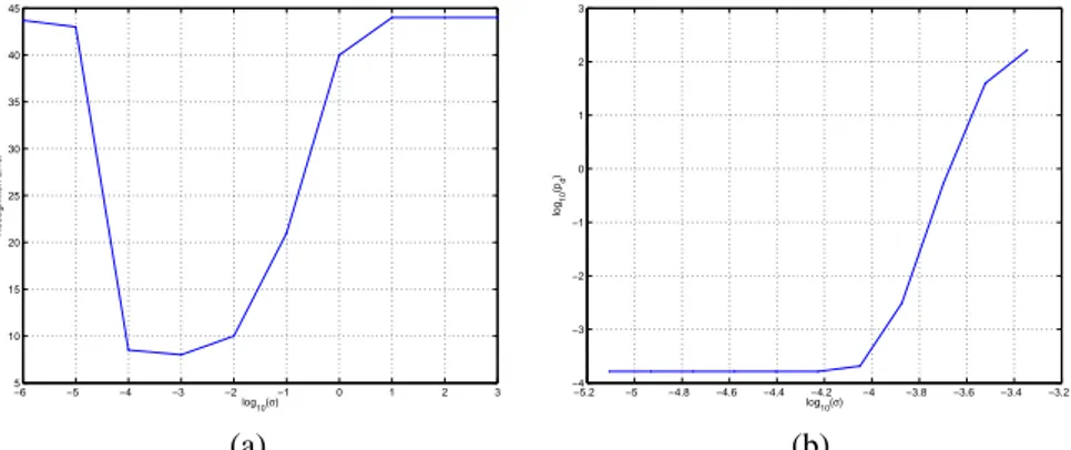
The tuning hyperparameter is chosen to be the scale factor σ in (2) of local kernel k. Although matching based kernel leads to a good performance, the Mercer condition in not usually insured. Fig. 2 presents ranked eigenvalues of the Gram matrix for different values of σ. For σ = 100, there exists negative eigenvalues of the Gram matrix, this means that matching kernel is not positive definite in general. By decreasing the scale σ, eigenvalues become always positive. Fig. 3-a shows the variation of the recognition error with respect to log10(σ). The optimal value obtained by cross-validation is σ∗ = 10−3
which corresponds to a positive definite Gram matrix (positive eigenvalues). Fig. 3-b represents the bound of probability pd(5) in a logarithmic scale with respect to log10(σ).
The probability confidence is set as η = 1 − 10−6. For the optimal choice of σ, the bound is very poor and useless. For σ = 10−4, which corresponds to a recognition error of 8%, we have pd ≤ 10−3. We can say for these values that Gram matrix is diagonally
dominant almost sure and so it is positive definite one. By choosing σ = 10−4we loose almost 5 % of recognition error which is not too much compared to the obtained warranty of convergence of the SVM algorithm to unique solution.
Figure 1: COIL-100 database with encrusted backgrounds, first raw: negative examples, second raw: positive examples.
Kernel Rec. Error
KS 23.49%
KM 9.58%
Kernel Rec. Error
KS 15.51 %
KM 3.08%
(a) (b)
20 40 60 80 100 120 140 0 20 40 60 80 100 i λi σ=10−3 σ=10−1 σ=1 σ=5 σ=10 σ=102 σ=103
Figure 2: Eigenvalues of Gram matrix for different σ.
−6 −5 −4 −3 −2 −1 0 1 2 3 5 10 15 20 25 30 35 40 45 log 10(σ) Recognition Error −5.2 −5 −4.8 −4.6 −4.4 −4.2 −4 −3.8 −3.6 −3.4 −3.2 −4 −3 −2 −1 0 1 2 3 log 10(σ) log 10 (pd ) (a) (b)
Figure 3: (a) Recognition error with respect to σ, (b) bound on pdwith respect to σ
Methods k-NN KH KM
Rec. Error 7.42 % 6.58 % 4.23%
Table 2: Global features ( k-NN, KH, 64 bins) vs Local feature (KM, 70 pts/image)
5
Conclusion
We have presented in this paper the use of matching kernels for SVMs in the context of object recognition. Despite the absence of an analytical proof of the Mercer property for such a kernel and the actual existence of counter examples, we have shown that we can choose kernel hyperparameter such that its Gram matrix is nevertheless positive definite with a very high probability. This criterion can be also used with advantages in many other applications where SVM approach applies, with local and global representations as well.
References
[1] Sch¨olkopf B. and Smola A. Learning with kernels. MIT University Press Cambridge, 2002. [2] C. Bahlmann, B. Haasdonk, and H. Burkhardt. On-line handwriting recognition with support
vector machines—a kernel approach. In Proc. of the 8th IWFHR, pages 49–54, 2002. [3] A. Barla, F. Odone, and A. Verri. Hausdorff kernel for 3d object acquisition and detection. In
In Proceedings of the European Conference on Computer Vision, LNCS 2353, page p. 20 ff,
2002.
[4] B. Caputo and Gy. Dorko. How to combine color and shape information for 3d object recog-nition: kernels do the trick. In Advances in Neural Information Processing Systems, 2002. [5] N. Cristianini and J. Shawe-Taylor. Support Vector Machines. Cambridge University Press,
2000.
[6] D. DeCoste and B. Sch¨olkopf. Training invariant support vector machines. In In Machine
Learning 46, pages 161–190, 2002.
[7] B. Sch¨olkopf et al. A kernel approach for learning from almost orthogonal patterns. In
Proceedings of the 13th European Conference on Machine Learning, 2002.
[8] J. Weston et al. Dealing with large diagonals in kernel matrices. In Spring Lecture Notes in
Computer Science 243.
[9] T. Gaertner. A survey of kernels for structured data. In IGKDD Explorations, 2003.
[10] V. Gouet, P. Montesinos, D., and Pel´e. Stereo matching of color images using differential in-variants. In Proceedings of the IEEE International Conference on Image Processing, Chicago, Etats-Unis, 1998.
[11] D. Haussler. Convolution kernels on discrete structures. In Technical Report UCS-CRL-99-10, 1999.
[12] R. Kondor and T. Jebara. A kernel between sets of vectors. In Proceedings of the ICML, 2003. [13] R. I. Kondor and J. Lafferty. Diffusion kernels on graphs and other discrete structures. In
Proceedings of the ICML, 2002.
[14] G. Lugosi. On concentration of measure inequalities. Lecture Notes, 1998.
[15] C. McDiarmid. On the method of bounded differences. London Mathematical Society Lecture
Note Series, 141(5):148–188, 1989.
[16] K. Mikolajczyk and C. Schmid. A performance evaluation of local descriptors. In CVPR, 2003.
[17] C. Schmid and R. Mohr. Local grayvalue invariants for image retrieval. IEEE Transactions
on Pattern Analysis and Machine Intelligence, 19(5):530–535, 1997.
[18] B. Sch¨olkopf. The kernel trick for distances. In NIPS, pages 301–307, 2000.
[19] C. Wallraven, B. Caputo, and A. Graf. Recognition with local features: the kernel recipe. In
ICCV, pages 257–264, 2003.
[20] C. Watkins. Dynamic alignment kernels. In Technical Report CSD-TR-98-11, 1999. [21] L. Wolf and A. Shashua. Kernel principal angles for classification machines with applications
to image sequence interpretation. In CVPR, 2003.
[22] Z. Zhang, R. Deriche, O. Faugeras, and Q. Luong. A robust technique for matching two uncal-ibrated images through the recovery of the unknown epipolar geometry. Artificial Intelligence, 78(1-2):87–119, 1995.