Stochastic Inventory Routing for Perishable Products

For Review Only

Stochastic inventory routing for perishable products

Journal: Transportation Science Manuscript ID TS-2016-0163.R1 Manuscript Type: Resubmitted Manuscripts Date Submitted by the Author: n/a

Complete List of Authors: Crama, Yves; University of Liege, HEC-Management School Rezaei, Mahmood; University of Liege, HEC-Management School Savelsbergh, Martin; Georgia Institute of Technology, Industrial and Systems Engineering

Van Woensel, Tom; Eindhoven University of Technology, Industrial Engineering

Keywords/Area of Expertise: inventory routing problem, perishable inventory system, stochastic inventory routing

For Review Only

Stochastic Inventory Routing for Perishable Products

HEC Liège, University of Liège, 4000 Liège, Belgium, y.crama@ulg.ac.be

Mahmood Rezaei

HEC Liège, University of Liège, 4000 Liège, Belgium, m.rezaei@ulg.ac.be

Martin Savelsbergh

School of Industrial and Systems Engineering, Georgia Institute of Technology Atlanta, GA 30332-0205, USA, martin.savelsbergh@isye.gatech.edu

Tom Van Woensel

School of Industrial Engineering, Eindhoven University of Technology, 5612AZ Eindhoven, Netherlands, t.v.woensel@tue.nl

Different solution methods are developed to solve an inventory routing problem for a perishable product with stochastic demands. The solution methods are compared empirically in terms of average profit, service level, and actual freshness. The benefits of explicitly considering demand uncertainty are quantified. The computational study highlights that in certain situations a simple ordering policy can already reach a very good performance, but that statistically and economically significant improvements are achieved when using more advanced solution methods. Managerial insights concerning the impact of shelf life and store capacity on profit are also obtained.

Key words: inventory routing problem; perishable inventory system; perishable inventory routing;

stochastic inventory routing.

History :

1.

Introduction

Consider a retail chain whose main goal is to optimize the long-term profit of a distribution network where products are shipped from a central warehouse (depot) to several stores. The decisions to be made are: (1) how much to deliver to each store in each period, and (2) which delivery routes to use. If customer demands at the stores are deterministic and known for the entire planning horizon, then this decision problem is known as the Inventory Routing Problem (IRP).

In this paper, we consider the IRP for a (single) perishable product, e.g., a dairy product, flowers, fruits, or vegetables, with stochastic customer demands. We develop and compare four solution methods: (1) an expected-value method in which stochastic demands are replaced by their expected values, (2) a deliver-up-to-level policy with a high target service level, (3) a decomposition method that relies on independent inventory control models for each store and on estimates of the routing 3 4 5 6 7 8 9 10 11 12 13 14 15 16 17 18 19 20 21 22 23 24 25 26 27 28 29 30 31 32 33 34 35 36 37 38 39 40 41 42 43 44 45 46 47 48 49 50 51 52 53 54 55 56 57 58 59

For Review Only

costs that can be attributed to each store, (4) a decomposition-integration method which improves the solution obtained by the decomposition method by analyzing and reducing the routing costs.

1.1. Motivation

In an IRP, both the delivery quantities at a store and the delivery routes to serve the stores are determined by a centralized decision-maker for a given planning horizon. IRPs are very difficult to solve to optimality even when the distribution network is small, far smaller than those typically encountered in practice. Coelho and Laporte (2014) report that instances of a single-product IRP with deterministic demands can rarely be solved to optimality when the number of stores exceeds 30. In contrast, a typical retail chain in Belgium (a small country) dispatches over 18,000 (perishable and dry) products from a central warehouse to more than 800 stores.

In most real-life IRP settings, demand experienced at stores is uncertain, giving rise to the more complex Stochastic IRP (SIRP). In such a setting, information regarding inventory levels at stores is periodically transmitted to the central warehouse, where a central decision-maker uses this infor-mation, and any available information about anticipated future demand, to determine the delivery quantities and the delivery routes for the next period, or the next few periods. When the actual demand from the customers at the stores is observed and updated inventory levels are transmitted to the warehouse, new next-period (or short-term) decisions are made. Due to the complexity of such a distribution system, retail chains frequently use a two-step decision-making process, in which each store deploys its own inventory management system to place orders (ignoring any impact these order placements may have on routing costs), and the centralized decision-maker uses a vehicle routing model to determine low-cost delivery routes to serve the placed orders. Such a two-step decision-making process does not necessarily yield an optimal profit for the retail chain, but offers a pragmatic approach for managing this complex system.

In many real-life IRP settings, product shelf life is not unlimited. Perishable products constitute over 52% of sales revenue of grocery retail chains (Chao et al. 2015), and roughly 10% of product is wasted before being sold (Kouki et al. 2015), while the food retail profit margin hardly exceeds 2%; see EBRD–FAO (2009), NAICS (2012), FMI (2014). Therefore, the profitability highly depends on efficient and effective inventory routing policies. The delivery frequency plays a major role in determining the profit, the service level, and the freshness. Indeed, infrequent deliveries of large delivery quantities reduces the routing costs, but also brings loss of freshness and a commensurate reduction in customer satisfaction (and possibly even lost sales due to the stochasticity of demand). Conversely, smaller quantities delivered more frequently improves freshness of products (and, con-sequently, ensures customer satisfaction) and reduces the risk of lost sales, but does imply higher routing costs. 3 4 5 6 7 8 9 10 11 12 13 14 15 16 17 18 19 20 21 22 23 24 25 26 27 28 29 30 31 32 33 34 35 36 37 38 39 40 41 42 43 44 45 46 47 48 49 50 51 52 53 54 55 56 57 58 59

For Review Only

In this paper, we study the stochastic inventory routing problem for a single perishable product (PSIRP) in which we seek to maximize profit subject to a given service level requirement. Even though freshness is considered and evaluated, it is not directly taken into account in the optimization.

1.2. Problem statement

Consider a generic retail chain that aims to maximize the expected net profit generated by the sales of a single perishable product. The net profit is measured by deducting acquisition, distribution, and other miscellaneous costs from the total revenue. Acquisition costs and revenue mostly depend on the quantities delivered to the stores, whereas distribution costs are also a consequence of the way the vehicles are dispatched. Miscellaneous costs are viewed as independent of either decision and are regarded as constant costs. As a result, we do not consider them in the objective function: the net profit is simply computed as (Revenue – Acquisition costs – Distribution costs), and its expected value defines the objective function.

Assume a finite planning horizon consisting of T consecutive periods. We consider an implicit complete graph G = (V, A), whose vertices represent the depot and the stores, and arcs represent the road segments between pairs of vertices. The travel cost from vertex i to vertex j is denoted as cij.

Product is picked up from the depot and delivered to the stores. Each route starts at the depot, ends at the depot, and cannot exceed a predefined length. The demand in period t from end customers at a store i is an integer random variable Dti(assuming independence for all periods and all stores) with

a known probability distribution. We define L to be the deterministic shelf life of the product from the arrival at the store. The acquisition cost of a unit of product is a. All units delivered in period t have the same selling price p during L periods. Unsold units perish at the end of period t + L− 1 with no salvage value. Unmet demand leads to lost sales but does not generate any other cost. The inventory holding cost is zero. We assume that the depot has an unlimited supply of product. The capacity of store i is denoted by Ci. The retail chain deploys a sufficiently large fleet of vehicles to

make deliveries, each with capacity Q. Each vehicle incurs a fixed cost K per period when it is used, and a variable cost equal to cij when traveling from vertex i to vertex j. Each store is served by at

most one vehicle in each period (no split deliveries).

The retail chain uses a centralized decision-making system to determine delivery quantities and routes in each period. The inventory state in store i at the beginning of period t is denoted by

Xti= (x1, x2, . . . , xL₋₁)ti, where (xk)ti is the inventory level of product with remaining shelf life k.

At the beginning of each period t, based on the inventory states, the retail chain decides about the delivery quantities, yti, and the delivery routes, Rt, to be used in the current period. There is no

time window for the delivery to stores, but in each period each vehicle performs at most one route with a predefined maximum length. The delivery lead time is zero, i.e., the delivery quantities yti

3 4 5 6 7 8 9 10 11 12 13 14 15 16 17 18 19 20 21 22 23 24 25 26 27 28 29 30 31 32 33 34 35 36 37 38 39 40 41 42 43 44 45 46 47 48 49 50 51 52 53 54 55 56 57 58 59

For Review Only

are available on the shelves at the beginning of period t, right after the decision is made. The real demand for period t is observed during the period and after quantity yti has been delivered. We

assume that the oldest units of product are sold first (FIFO issuing policy), i.e., (xk)ti is stored until

(xk−1)ti is used up or perished.

A predefined Target Service Level (T SL) must be respected in every period and in every store. More precisely, the total inventory available in store i in period t must be such that the probability of not incurring a stockout in period t is at least equal to T SL. In practice, the average service level of perishables is estimated to be around 92% in Europe and the USA (Minner and Transchel 2010).

All notation is summarized in Table 1.

Table 1 Indices, parameters, and decision variables

Indices:

i, j indices for vertices (depot and stores)

k index for remaining shelf life

r index for routes

t index for periods

Parameters:

T length of the planning horizon

N number of stores

L shelf life of the product

T SL target service level to be respected in every period and in each store

a acquisition price of each unit of the product

p selling price of each unit of the product

Ci capacity of store i

(xk)ti inventory level with remaining shelf life k in period t in store i before delivery

(x1, x2, . . . , xL−1)ti state of the system in period t in store i before delivery

Iti total inventory level in period t in store i before delivery

Dti random demand of end customers in period t in store i (integer-valued)

P r(Dti= d) probability function of demand in period t in store i

Q capacity of each vehicle

cij distance and travel cost from vertex i to vertex j

K fixed cost of using a vehicle

Fti estimated cost-to-serve assigned in period t to store i

Decision variables:

yti delivery quantity in period t to store i (integer values)

Rt set of routes used in period t (index r)

π expected profit generated by all stores over the planning horizon

1.3. Scientific contributions

As outlined above, we investigate a stochastic inventory routing problem for a single perishable product. Our main contributions are:

3 4 5 6 7 8 9 10 11 12 13 14 15 16 17 18 19 20 21 22 23 24 25 26 27 28 29 30 31 32 33 34 35 36 37 38 39 40 41 42 43 44 45 46 47 48 49 50 51 52 53 54 55 56 57 58 59

For Review Only

• The development of four different solution methods for the PSIRP. The methods differ in sophis-tication and emphasis placed on features of the problem, e.g., perishability of the product, stochas-ticity of the demand, or target service level. The decomposition method and the decomposition-integration method, presented in Sections 5–7, rely on an original combination of stochastic dynamic programming and combinatorial optimization techniques.

• The analysis of the results of an extensive computational study, which establishes the relative performance of the solution methods (and the influence of their parameter settings) for different classes of instances and on different metrics of interest, e.g., total profit, average freshness, and sim-plicity of implementation. Among others, we demonstrate that a simple, easy-to-implement replen-ishment policy, derived from one of the more sophisticated solution methods, is highly effective in a variety of settings.

• The creation of managerial insights related to the impact of store capacity and shelf life on the expected profit.

The remainder of the paper is organized as follows. In Section 2, an extensive literature review is presented. Sections 3–6 introduce the four solution methods, two elementary methods and two sophisticated methods. In Section 7, we develop a matheuristic to solve an optimization subproblem arising in our most sophisticated solution method. Section 8 presents a heuristic algorithm for the case in which full information is available regarding future demand is available (which will be used for comparison purposes in the computation study). Section 9 discusses the setup of our comprehen-sive computational study. Results of the computational experiments are presented and analyzed in Section 10. Finally, concluding remarks are given in Section 11.

2.

Literature review

Inventory-routing models naturally relate to various management practices, and in particular, to vendor-managed inventory (VMI) and to retailer-managed inventory (RMI) systems. The VMI approach relies on cooperation and on information sharing between a supplier and its customers. When VMI is implemented, the supplier takes over the responsibility of managing the inventory of the customers by deciding on replenishment quantities and delivery periods. The consequences can be beneficial for both parties: customers need to employ less resources for controlling their inventory, and the supplier has more flexibility for integrating the replenishment quantities and periods to dif-ferent customers (Desaulniers et al. 2016). In contrast, in an RMI system, the customers decide when and how much to order, independently of each other, so that the ability of the supplier to optimize its transportation costs is strongly restricted by the customers’ decisions (Archetti and Speranza 2016, Bertazzi and Speranza 2012).

3 4 5 6 7 8 9 10 11 12 13 14 15 16 17 18 19 20 21 22 23 24 25 26 27 28 29 30 31 32 33 34 35 36 37 38 39 40 41 42 43 44 45 46 47 48 49 50 51 52 53 54 55 56 57 58 59

For Review Only

The (classical) IRP deals with deterministic demands and is concerned with the distribution of a single product from a single depot to a set of customers with deterministic demands over a given planning horizon. The objective is to minimize the distribution and inventory costs during the planning period without causing stock-outs at any of the customers. As in a VMI system, the main decisions in an IRP are: (a) when to serve each customer, (b) how much to deliver to a customer when it is visited, and (c) which routes to use. The IRP has a wide range of applications including the distribution of gas (Campbell and Savelsbergh 2004a, Gronhaug et al. 2010), fuel (Popović et al. 2012), automobile components (Alegre et al. 2007, Stacey et al. 2007), perishable products (Federgruen and Zipkin 1984, Federgruen et al. 1986), groceries products (Gaur and Ficher 2004), cement (Christiansen et al. 2011), and blood products (Hemmelmayr et al. 2009).

Since the IRP has the flexibility to decide how much to deliver to each customer and which routes to use in each period, the decision space becomes enormously large even when compared, for instance, with classical vehicle routing problems (VRP). Exact approaches are typically based on mixed integer programming (MIP) formulations using arc-flow decision variables, although route-based formulations have also been used (Desaulniers et al. 2016). But finding the optimal solution of such models is quite challenging, even for very small instances of the IRP (Campbell et al. 1998). Therefore, many early algorithms proposed in the literature decompose the IRP into two stages: (a) inventory control (determining the delivery amounts), and (b) vehicle routing (Campbell and Savelsbergh 2004b, Federgruen and Zipkin 1984, Qu et al. 1999). In some cases, an overall solution is found by iterating between these two problems (Federgruen and Zipkin 1984, Qu et al. 1999). Exact algorithms for the IRP are more recent. They include the branch-and-cut algorithms of Coelho and Laporte (2013a), Coelho and Laporte (2013b), and Coelho and Laporte (2014d), and the branch-and-price-and-cut algorithm of Desaulniers et al. (2016).

Researchers have also striven to develop solution methods for simplified versions of IRP models, rather than the classical IRP model. Examples of simplifying assumptions include:

• deliver-up-to-level (UL) replenishment policies; Bertazzi et al. (2002), Archetti et al. (2007), Solyali and Süral (2011);

• direct delivery policies; Bertazzi and Speranza (2012);

• deliveries occurring only when inventory levels are down to zero; Chan et al. (1998) and Jaillet et al. (2002);

• single vehicle; see, e.g., Archetti et al. (2007) and Solyali and Süral (2011);

• constant demand rate over time; Raa and Aghezaaf (2008, 2009), Ekici et al. (2015); • periodic deliveries; Bertazzi and Speranza (2012), Campbell and Wilson (2014).

Andersson et al. (2010), Bertazzi and Speranza (2011, 2012, 2013) and Coelho et al. (2014) provide excellent reviews on IRPs, both from the application and the methodological points of view.

3 4 5 6 7 8 9 10 11 12 13 14 15 16 17 18 19 20 21 22 23 24 25 26 27 28 29 30 31 32 33 34 35 36 37 38 39 40 41 42 43 44 45 46 47 48 49 50 51 52 53 54 55 56 57 58 59

For Review Only

In the stochastic inventory routing-problem (SIRP), future customer demands are uncertain, and are given by their probability distributions. While the majority of papers on the SIRP assume that demands are fully realized at the end of each period, some models assume that demands are realized upon arrival of the vehicle at a customer (Berman and Larson 2001, Huang and Lin 2010).

Demand stochasticity implies that shortages may occur, and there is often a positive probability that a customer runs out of stock. To restrict shortages, a penalty is imposed whenever a customer runs out of stock, and this penalty is usually taken to be proportional to the unsatisfied demand. Unsatisfied demand is typically considered to be lost sale (Minkoff 1993, Kleywegt et al. 2004), and is rarely dealt with as backlogging, as in the work by Yu et al. (2012). In either case, penalties may apply. A pre-defined service level may apply too, which imposes a minimum inventory level at each customer in each period (Yu et al. 2012). The objective is to choose a delivery policy that minimizes the expected total (inventory, distribution and penalty) costs per period. Due to the complexity of the SIRP, simplifying assumptions are frequently made, as in the IRP. These assumptions may include considering a single capacitated vehicle (Coelho and Laporte 2014, Reinman et al. 1999, Schwartz et al. 2006), a single uncapacitated vehicle (Qu et al. 1999), or direct deliveries (Barnes-Schuster and Bassok 1997, Kleywegt et al. 2002, Reinman et al. 1999).

Markov decision processes (MDP) can be used to model SIRPs over an infinite planning horizon. MDP models formulate a value function which depends on inventory levels. When the demand probability distribution is stationary, a deterministic optimal policy can be calculated for each state, and the value function can be optimized by standard techniques such as policy iteration, value iteration, or successive approximation. These algorithms are practical only if the state space is small and if the optimization problem can be solved efficiently. None of these requirements are satisfied by real-world instances of the SIRP, as the state space is usually extremely large, even if inventories are discretized, and the optimization problem includes a vehicle routing problem as a special case (Campbell et al. 1998). Due to the curse of dimensionality, researchers often use approximations of the value function (Minkoff 1993, Adelman 2004) or decompose it (Kleywegt et al. 2004). Based on the LP model proposed by Puterman (1994), Adelman (2004) formulates and interprets two primal-dual approximations. Such approximations relax the feasible region of the dual problem, and so provide upper bounds on the original dual maximization problem. Kleywegt et al. (2004) formulate an MDP model of the SIRP and propose approximation methods to find good solutions within reasonable time. This is the extension of an earlier paper (Kleywegt et al. 2002) in which the authors formulated an SIRP with direct deliveries as an MDP and proposed an approximate dynamic programming approach for its solution.

3 4 5 6 7 8 9 10 11 12 13 14 15 16 17 18 19 20 21 22 23 24 25 26 27 28 29 30 31 32 33 34 35 36 37 38 39 40 41 42 43 44 45 46 47 48 49 50 51 52 53 54 55 56 57 58 59

For Review Only

Solution methods other than MDP have also been used for solving SIRPs. In Jaillet et al. (2002), for instance, long-term delivery costs are incorporated into shorter planning horizons. In Yu et al. (2012), rather than dealing with an exact stochastic model, an approximate SIRP model is proposed and transformed into a simplified deterministic one. Then, Lagrangian relaxation is used to decompose the model into an inventory problem and a vehicle routing problem.

2.3. Inventory-routing for perishables

The IRP for perishables (PIRP) is identical to the classical IRP, except that products have a limited shelf life after which they lose their value. In the deterministic case, shortages are not allowed. Moreover, thanks to the complete knowledge of demand, no products need to deteriorate. This implies that the cost components in the PIRP are the same as for non-perishables, i.e, total inventory holding costs and routing costs over the planning horizon. The main difference with the classical IRP is that the deliveries to customers are now restricted by the maximum shelf life of the product. As a consequence, delivery frequency plays an important role. Less frequent deliveries reduce the routing costs, but result in more units with short remaining shelf lives in the following periods; these units are subject to holding cost and to deterioration, and their sales may be reversely affected by their lack of freshness. Therefore, finding a right trade-off between costs and freshness is crucial. The main objective in most applications is to minimize costs (or to maximize profit), while freshness is controlled by imposing additional side constraints on delivery quantities. Hemmelmayr et al. (2009) investigate the delivery of blood products to hospitals, where the tour length is restricted, but vehicle capacity is ignored in view of the small size of blood bags, and no inventory cost is imposed. The objective is to minimize travel costs over a finite horizon. The authors develop and evaluate two delivery strategies, namely: (1) using fixed routes but deciding about delivery days, and (2) repeating delivery patterns for each hospital. Coelho and Laporte (2014) consider age-dependent holding costs and selling prices in a PIRP, where the supplier has the choice to deliver either fresh or aged products, and each case yields different holding costs and revenues. The objective function maximizes the total sales revenue, minus inventory and routing costs. Le et al. (2013) propose a mathematical model based on feasible routes that start from the depot, visit a subset of stores at most one time, and then return to the depot, without the necessity of respecting the vehicle capacity. The objective function represents the sum of transportation costs and inventory costs. They use a column-generation based algorithm to solve the problem. Their work is extended by Al Shamsi et al. (2014) to include the cost of CO2 emissions, based on the vehicle load and distance. The resultant model is an MINLP

problem which is solved using a commercial solver. In Mirzaei and Seifi (2015), dependency of the end-customers demand on the age of the inventory is formulated as a PIRP so that a portion of the demand is considered as lost sale if inventory is not as fresh as it could be. The objective function is the total cost of transportation, lost sale, and holding inventories. The authors develop a hybrid simulated annealing and tabu search algorithm for solving the problem.

3 4 5 6 7 8 9 10 11 12 13 14 15 16 17 18 19 20 21 22 23 24 25 26 27 28 29 30 31 32 33 34 35 36 37 38 39 40 41 42 43 44 45 46 47 48 49 50 51 52 53 54 55 56 57 58 59

For Review Only

Recall that in an RMI system, the stores decide when and how much to order, independently of each other. Therefore, the main decision variables in an RMI perishable inventory system are the order time and the order quantity. To place an order, the current inventory level and age of the stocked products (state of the system) are observed. In most problem settings, an MDP provides an exact solution approach. However, the computation of the optimal order for every state of the system using classical techniques is in general intractable because of the curse of dimensionality. Thus, many researchers turned to effective heuristic policies to handle these problems, mostly for the case of independent and identically distributed demands (Chao et al. 2015). The most widely used periodic-review ordering policies are (R, S) (Chiu 1995, Cooper 2001, Deniz et al. 2010) and (R, s, S) (Broekmeulen and Van Donselaar 2009, Lian and Liu 1999), where R refers to the number of periods between two consecutive reviews of the inventory system, s denotes the inventory level below which an order is triggered, and S is the order-up-to level value. When demands are stochastic, obtaining optimal parameters in periodic-review policies even for a single perishable product with deterministic shelf life is notoriously complicated. The fixed shelf life perishability problem remains complex when the product lifetime is longer than two units of time in a periodic review system (Kouki and Jouini 2015). Hence, researchers have worked on approximating outdate costs (Broekmeulen and Van Donselaar 2009, Chiu 1995) or calculating upper and lower bounds on the number of outdates (Chiu 1995, Cooper 2001). Some models deal with batch demands (Lian and Liu 1999) or batch orders (Broekmeulen and Van Donselaar 2009). Finally, service level is regarded as a constraint in some papers including Adachi et al. (1999), Broekmeulen and Van Donselaar (2009), and Minner and Transchel (2010). The interested reader is referred to Goyal and Giri (2001), Karaesmen et al. (2011), and Nahmias (2011), for the review works on perishables.

In conclusion, the IRP and its variants are complex problems. Considering perishable products and stochastic demands complicates the model even further. As a result, applying existing solution methods is mathematically very difficult and computationally very inefficient.

3.

The expected value method

A classical way to reduce the complexity of stochastic models is to replace random variables by their expected values. Unfortunately, even deterministic IRPs are extremely difficult to solve (see, e.g., Coelho and Laporte (2014)), which is why we settle here for a simple heuristic solution. The expected

value method (EV ) provides a first benchmark.

In EV , all demands are deterministic, given by E(Dti), for all i, t. In a first step, each store

independently determines its delivery quantities. Under these assumptions, the inventory control problem of a store can be viewed as a lot sizing problem where routing induces an implicit ordering 3 4 5 6 7 8 9 10 11 12 13 14 15 16 17 18 19 20 21 22 23 24 25 26 27 28 29 30 31 32 33 34 35 36 37 38 39 40 41 42 43 44 45 46 47 48 49 50 51 52 53 54 55 56 57 58 59

For Review Only

cost. The exact routing costs are determined in a second step. Hence, it is optimal for each store to place as few orders as possible while satisfying demand.

More specifically, assume that the inventory levels in period t in store i before delivery are given as (x1, x2, . . . , xL−1)ti, so that the total inventory level is

Iti= L−1

∑

k=1

(xk)ti. (1)

At the beginning of period t, for each store i, EV determines the delivery quantity as follows: if the current inventory level Itiis larger than or equal to the expected demand E(Dti), the delivery quantity

is zero. Otherwise, EV delivers enough to satisfy the expected demands of L periods, including the current period, provided that store capacity Ci is respected. Then, a VRP based on these delivery

quantities is solved and implemented, real demands are observed, new inventory levels are calculated for the next period, and the same decision making process is repeated in period t + 1.

All necessary computations can be carried out as follows. Assume that in period t, yti units are

delivered to store i and the actual demand observed in store i is dti. Then, the inventory level of

the store in period t + 1 is determined by relation (3), where (z)+_{= max(z, 0) and (x}

L)ti= yti by convention: ((x1, x2, . . . , xL₋₁)ti, yti) dti → (x1, x2, . . . , xL₋₁)t+1,i (2) (xk)t+1,i= ((xk+1)ti− (dti− k ∑ l=1 (xl)ti)+)+, for k = 1, . . . , L− 1. (3)

The algorithm is summarized as follows.

The expected value algorithm (EV ) Begin

Step 0. Set t = 1.

Step 1. For each store i, if Iti≥ E(Dti), set yti= 0; otherwise, set yti= min{Ci− Iti, ⌊E(Dti) +

. . . + E(Dt+L−1,i)⌋ − Iti}.

Step 2. Solve a VRP for the delivery quantities yti’s and serve the stores through the optimal VRP

routes.

Step 3. For each store i, observe the actual demand in period t, say dti. Calculate the state of the

system in period t + 1, i.e., Xt+1,i by Relations (3). Set t = t + 1 and go to Step 1.

End

In each period t and store i, the expected value method can be viewed as an (R, s, S) policy, where

R = 1, s = E(Dti), and S = min{Ci, ⌊E(Dti) + . . . + E(Dt+L_−1,i)⌋}.

3 4 5 6 7 8 9 10 11 12 13 14 15 16 17 18 19 20 21 22 23 24 25 26 27 28 29 30 31 32 33 34 35 36 37 38 39 40 41 42 43 44 45 46 47 48 49 50 51 52 53 54 55 56 57 58 59

For Review Only

4. A deliver-up-to-level method

Another simple heuristic is obtained by replacing Step 1 of the EV algorithm with a replenishment rule that explicitly takes into account the stochasticity of demand. More specifically, for any λ_{≤ L,} let us denote by qti(λ) the smallest integer quantity which suffices to meet the demand at store i during

λ consecutive periods{t, . . . , t + λ − 1} with probability T SL: P r(Dti+· · · + Dt+λ_−1,i≤ q

(λ)

ti )≥ T SL, (4)

and consider the deliver-up-to-level method U Lλ.

The deliver-up-to-level algorithm (U Lλ)

Begin

Step 0. Set t = 1.

Step 1. For each store i, if P r(Dti≤ Iti)≥ T SL, set yti= 0; otherwise, set yti= min{Ci− Iti, q

(λ)

ti −

Iti}.

Step 2. Solve a VRP for the delivery quantities yti and serve the stores through the optimal VRP

routes.

Step 3. For each store i, observe the actual demand in period t, say dti. Calculate the state of the

system in period t + 1, i.e., Xt+1,i, by Relations (3). Set t = t + 1 and go to Step 1.

End

The algorithm U Lλ (greedily) sets yti= 0 whenever Iti suffices to satisfy T SL in period t, since

a positive delivery quantity would increase the routing costs in period t. If the inventory does not suffice to satisfy T SL in period t, U Lλdelivers a quantity ytiwhich should be sufficient to satisfy the

demand in the next λ periods, unless the required quantity would exceed the store capacity Ci. So,

U Lλ acts like an (R, s, S) policy where sU L= q

(1)

ti , SU L= min{Ci, q

(λ)

ti }, and R = 1 so as to enforce

T SL in every period. Note that λ = 1 tends to provide the freshest products on shelf, thanks to daily

deliveries, whereas bigger values of λ yield lower routing costs and possibly higher profit.

5. A decomposition method

The deliver-up-to-level method U Lλ focuses on the target service level in order to determine the

delivery quantities, and mostly ignores the importance of revenues and routing costs. Our next methods rely on a Stochastic Dynamic Programming (SDP) model, which explicitly account for these aspects.

In the SDP model, the state of the system in period t is defined by the inventory levels in all stores, i.e., ((x1, . . . , xL₋₁)t1, . . . , (x1, . . . , xL₋₁)tN). The decision variables are the delivery quantities

3 4 5 6 7 8 9 10 11 12 13 14 15 16 17 18 19 20 21 22 23 24 25 26 27 28 29 30 31 32 33 34 35 36 37 38 39 40 41 42 43 44 45 46 47 48 49 50 51 52 53 54 55 56 57 58 59

For Review Only

in period t, i.e., (yt1, . . . , ytN), and the routing decisions. Given a decision on delivery quantities

in period t, the direct costs (acquisition and routing) as well as the expected revenue in period t can be formulated, as well as the potential states of the system in period t + 1 and the transition probabilities. Theoretically, one can set SDP relations to determine the optimal delivery quantities in each period based on the state of the system. However, this can only be applied to very small-size instances. Considering N stores, a maximum shelf life L, and inventory levels to be integers in the interval [0, C], there are (C + 1)N (L_{−1) potential states in each period. Therefore, it is necessary to}

resort to heuristic methods to solve even small instances through SDP.

We solve an independent SDP for each store, aiming to optimize an estimate of the store’s expected revenue over the planning horizon. Although such a decomposition yields sub-optimal solutions, the complexity no longer depends exponentially on the number of stores. The number of states in each period for each store is (C + 1)(L−1)_{, which is computationally tractable for small values of L. In}

each period, the SDP relations allow us to determine a delivery quantity to each store, based on its current inventory level, while neglecting the routing costs. Then, we solve a VRP to obtain optimal routes for these delivery quantities. We call this the decomposition method (DE).

Since the SDP model considers each store independently, it does not properly account for the routing costs. Therefore, in the model associated with store i, we charge a fixed cost-to-serve Fti if

the store is visited in period t. This cost-to-serve acts as a proxy for the routing cost for delivery to store i. The choice of Fti is discussed later.

Define Xti=

(

(x1)ti, . . . , (xL−1)ti

)

, Xt= (Xt1, . . . , XtN), and Yt= (yt1, . . . , ytN), so that (Xt, Yt)

denotes the complete state of the system at time t after the quantities yt1, . . . , ytN have been delivered.

Define fti(Xti, yti) as the total expected profit for store i from period t until the end of the planning

horizon when the state of the store is Xti and the delivery quantity is yti. The function fti includes

total revenue, acquisition costs, and the cost-to-serve. The optimal expected profit generated by store i from period t to the end of the horizon is denoted f_ti∗(Xti), that is,

f_ti∗(Xti) = max y(1)_ti ≤yti≤Ci−Iti

fti(Xti, yti), (5)

where y(1)

ti is the smallest integer satisfying Inequality (4). The optimal delivery quantity is specified

by Equation (6): yti∗ = yti∗(Xti) = arg max y(1)_ti ≤yti≤Ci−Iti fti(Xti, yti). (6) 3 4 5 6 7 8 9 10 11 12 13 14 15 16 17 18 19 20 21 22 23 24 25 26 27 28 29 30 31 32 33 34 35 36 37 38 39 40 41 42 43 44 45 46 47 48 49 50 51 52 53 54 55 56 57 58 59

For Review Only

In order to determine the optimal delivery quantity y_ti∗, we solve the recursive Equations (7) by backward induction: fti(Xti, yti) =−Fti·1(yti> 0)− ayti + P r(Dti> Iti+ yti) ( p(Iti+ yti) + ft+1,i∗ (0, . . . , 0, 0) ) + Iti∑+yti d=0 P r(Dti= d) ( pd + ft+1,i∗ (Xt+1,i) ) (7)

where Xt+1,i= (x1, . . . , xL₋₁)t+1,i is defined by Equation (3). The first term in Equation (7) is an

estimate of the routing cost incurred to serve store i; the second term is the acquisition cost of yti

units; the third term accounts for the expected revenue collected from store i when the demand in period t is larger than the inventory available at i in period t, and for the expected profit in periods

t + 1, . . . , T ; similarly, the last term expresses the expected revenue in period t and the expected

profit in periods t + 1, . . . , T when the demand does not exceed the available inventory. In order to solve (7), we use the boundary condition:

fT +1,i∗ ((x1, x2, . . . , xL−1)T +1,i) =

a

2IT +1,i, (8)

where the right-hand side of (8) is an estimate of the profit generated by the inventory left over at the end of the horizon.

The decomposition algorithm is as follows.

The decomposition algorithm (DE) Begin

Step 0. Set a cost-to-serve, Fti, for each store i and each period t based on one of the algorithms

described in Appendix A. Set t = 1.

Step 1. Use Equations (6)–(7) to determine a delivery quantity to each store i in period t, say y_ti∗, given the state of the system Xti= (x1, . . . , xL−1)ti.

Step 2. Solve a VRP for the delivery quantities y_ti∗ and serve the stores through the optimal VRP routes.

Step 3. For each store i, observe the actual demand in period t, say dti. Calculate the state of the

system in period t + 1, i.e., Xt+1,i by Relations (3). Set t = t + 1 and go to Step 1.

End

The DE algorithm can yield adequate solutions for the PSIRP provided that the costs-to-serve Fti

are reliable estimates of the actual routing costs. For symmetric travel costs satisfying the triangle inequality, a natural range for the cost-to-serve of store i is [0, K + 2ci0], where the upper bound

3 4 5 6 7 8 9 10 11 12 13 14 15 16 17 18 19 20 21 22 23 24 25 26 27 28 29 30 31 32 33 34 35 36 37 38 39 40 41 42 43 44 45 46 47 48 49 50 51 52 53 54 55 56 57 58 59

For Review Only

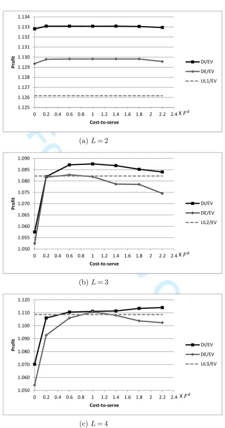
represents the cost of a direct delivery to store i. When we set Fti= 0 for all stores, we obtain an

algorithm that we call DE0. This leads to a high delivery frequency. It provides very fresh products

but ignores, and, implicitly increases, the routing costs. When the delivery quantity is close to the vehicle capacity Q, no other store can be served on the same route, and Fti= K + 2ci0is the correct

routing cost. In this case, each store can be dealt with independently.

When more than one store is served by each route, neither Fti= 0 nor Fti= K + 2ci0 proves to be

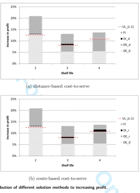
a good setting. In Appendix A, we introduce two methods to calculate an intermediate cost-to-serve to be assigned to each store. The first approach yields a distance-based cost-to-serve Fd

tiwhich focuses

on the average distance between each store and its closest neighbors. The second approach produces a route-based cost-to-serve Fr

ti which allocates the total cost of a route to the stores it includes.

6.

A decomposition-integration method

In this section, we improve our estimate of the expected profit given in Equation (7), by taking into account the actual routing costs in period t and by refining the approximation of the routing costs in period t + 1 (as compared to the costs-to-serve Fti). The values Fti are still used from period

t + 2 onward. Note that given the state of the system at time t, say Xt, and the vector of delivery

quantities denoted by Yt, a first estimate of the total profit for periods t to T is simply obtained as:

π1t(Xt, Yt) = N ∑ i=1 fti(Xti, yti) = N ∑ i=1 fti((x1, . . . , xL−1)ti, yti). (9)

Now, let R(y1, . . . , yN) represent the optimal routing cost with delivery quantities (y1, . . . , yN). Then,

Equation (9) can be improved by replacing the fixed costs-to-serve by the true routing cost in period t. This leads to:

π2 t(Xt, Yt) = N ∑ i=1 fti(Xti, yti) + N ∑ i=1 Fti·1(yti> 0)− R(yt1, . . . , ytN). (10)

In order to apply a similar correction to the routing costs for period t + 1, denote by y+

t+1,1, . . . , y

+

t+1,N

the optimal delivery quantities in period t + 1. Note that these quantities depend in a complex way on (Xt, Yt) and are actually random variables, since they also depend on the realization of the demands

Dt1, . . . , DtN in period t. With these notations, another estimate of the total expected profit can be

derived from Equation (10), as follows:

π3t(Xt, Yt) = N ∑ i=1 fti((x1, . . . , xL₋₁)ti, yti) + N ∑ i=1 Fti·1(yti> 0)− R(yt1, . . . , ytN) + N ∑ i=1 Fti· P r(y+t+1,i> 0| Yt) − ∑ (y1,...,yN) P r((yt+1,1+ , . . . , y + t+1,N) = (y1, . . . , yN)|Yt)× R(y1, . . . , yN). (11) 3 4 5 6 7 8 9 10 11 12 13 14 15 16 17 18 19 20 21 22 23 24 25 26 27 28 29 30 31 32 33 34 35 36 37 38 39 40 41 42 43 44 45 46 47 48 49 50 51 52 53 54 55 56 57 58 59

For Review Only

In this expression, the fourth term corrects the expected value of the cost-to-serve in period t + 1, and the last term represents the expected value of the routing cost in period t + 1, given the delivery decisions Yt.

The optimal delivery quantity y+

t+1,i can be approximated by the expected value of yt+1,i∗ . Based

on Equation (6), this can be estimated as follows (compare with Equation (7)):

E(yt+1,i∗ | yti) = P r(Dti> Iti+ yti) y∗t+1,i(0, . . . , 0, 0)

+

Iti∑+yti

d=0

P r(Dti= d) yt+1,i∗ (Xt+1,i)

(12)

where Xt+1,i is defined by Equation (3).

Replacing the random quantities y+

t+1,i by ⌊E(yt+1,i∗ | yti)⌋ turns (11) into a deterministic problem

where the delivery cost in period t + 1 can be approximated by solving a single VRP. This approach has the drawback, however, of yielding strictly positive values ⌊E(y∗_t+1,i| yti)⌋ for almost all stores

i, which is unlikely to happen for the optimal delivery quantities y_t+1,i∗ because this would result in high routing costs. Therefore, we further modify our approximation by considering delivery quantities (˜yt+1,i| yti) defined by Equation (13) hereunder, where ϵi is a user-parameter whose value depends

on the magnitude of the demand (ϵi=1₂E(Dit) proved suitable in our numerical experiments):

(˜yt+1,i|yti) =

{

⌊E(y∗

t+1,i|yti)⌋ if ⌊E(y∗t+1,i|yti)⌋ > ϵi,

0 otherwise. (13)

The optimal expected total profit is then approximated by solving the optimization problem (14).

max (yt1,...,ytN) ˜ π(yt1, . . . , ytN) = N ∑ i=1 fti((x1, x2, . . . , xL−1)ti, yti) + N ∑ i=1

Fti· (1(yti> 0) +1((˜yt+1,i|yti) > 0))

− R(yt1, . . . , ytN)− R((˜yt+1,1|yt1), . . . , (˜yt+1,N|ytN))

subject to y(1)ti ≤ yti≤ Ci− Iti, i = 1, . . . , N.

(14)

This formulation takes into account the routing costs in period t, the approximated expected routing costs in period t + 1, and costs-to-serve for the following periods. The corresponding algorithm is summarized as follows:

The decomposition-integration algorithm (DI) Begin

Step 0. Set a cost-to-serve, Fti, for each store i and each period t based on one of the algorithms

described in Appendix (A). Set t = 1. 3 4 5 6 7 8 9 10 11 12 13 14 15 16 17 18 19 20 21 22 23 24 25 26 27 28 29 30 31 32 33 34 35 36 37 38 39 40 41 42 43 44 45 46 47 48 49 50 51 52 53 54 55 56 57 58 59

For Review Only

Step 1. Solve Problem (14) to obtain the delivery quantities yti and the corresponding routes in

period t.

Step 2. Serve the stores with the delivery quantities yti through the routes obtained in Step 1. Step 3. For each store i, observe the actual demand in period t, say dti. Calculate the state of the

system in period t + 1, i.e., Xt+1,i by Relations (3). Set t = t + 1 and go to Step 1.

End

In the next section, we propose a matheuristic algorithm to solve Problem (14), as required by Step 1 of Algorithm DI.

7.

A matheuristic for Problem (14)

In this section, we propose a matheuristic for Problem (14).

Starting from the initial solution Yt= (y∗t1, . . . , ytN∗ ) proposed by Equation (6), we generate a new

feasible solution Y_t′ = (y′t1,· · · , y

′

tN) as explained below, and we explore whether ˜π(Y

′

t) is larger

than ˜π(Yt). If so, we move to the new solution; otherwise, we generate another solution. The local

improvement algorithm stops when a pre-defined number of consecutively generated new solutions are rejected due to either lack of improvement or infeasibility. Calculating_{eπ in Problem (14) for any} new solution involves solving two VRPs. In order to avoid these expensive computations, each new solution is not generated randomly but in a systematic way which allows us to recompute ˜π(Yt′)

incrementally, by difference with ˜π(Yt).

When moving from the current solution (the current set of delivery quantities and their optimal routes) to a new solution, the difference in the approximated expected total profit is calculated by Equation (15): ∆ =eπ(y′t1, y ′ t2, . . . , y ′ tN)−eπ(yt1, yt2, . . . , ytN) = N ∑ i=1 (fti((x1, x2, . . . , xL₋₁)ti, y ′ ti)− fti((x1, x2, . . . , xL₋₁)ti, yti)) − (R(yt1′ , . . . , y ′ tN)− R(yt1, . . . , ytN)) − (R((˜yt+1,1′ |y ′ t1), . . . , (˜y ′ t+1,N|y ′ tN))− R((˜yt+1,1|yt1), . . . , (˜yt+1,N|ytN))) + N ∑ i=1 Fti· (1(y ′ ti> 0)−1(yti> 0)) + N ∑ i=1 Fti· (1((˜y ′ t+1,i|y ′ ti) > 0)−1((˜yt+1,i|yti) > 0)). (15)

Assume that in every move from the current solution to a new solution, we change the delivery quantities in such a way that the routes, and so the routing costs, in period t + 1 do not change. Moreover, let us indicate the decrease in the routing costs in period t by δ:

δ = R(yt1, . . . , ytN)− R(y ′ t1, . . . , y ′ tN). (16) 3 4 5 6 7 8 9 10 11 12 13 14 15 16 17 18 19 20 21 22 23 24 25 26 27 28 29 30 31 32 33 34 35 36 37 38 39 40 41 42 43 44 45 46 47 48 49 50 51 52 53 54 55 56 57 58 59

For Review Only

Then, one can rewrite Equation (15) as follows: ∆ = N ∑ i=1 (fti((x1, x2, . . . , xL₋₁)ti, y ′ ti)− fti((x1, x2, . . . , xL₋₁)ti, yti)) + δ + N ∑ i=1 Fti· (1(y ′ ti> 0)−1(yti> 0)). (17)

In the proposed matheuristic, a new solution is generated in such a way that the routing cost in period t decreases while the expected routing cost in period t + 1 does not change. We explain the main idea here.

Assume that in period t, a store j is ejected from its current route and is inserted into another route, say route r∗, without modification of the delivery quantities Yt. Denote by r′ the route in

period t derived from route r∗ _{after inserting store j into it. If route r}′ _{is feasible for the delivery}

quantities Yt and if the routing cost in period t decreases as a result of this ejection-insertion step,

then, clearly, the new VRP solution is preferred to the previous one. Generally speaking, however, since the routes were optimally selected for the delivery quantities Yt, route r′will be infeasible either

with respect to its maximum allowed length or with respect to the capacity of the vehicle. In the first case, we simply reject the new solution. In the second case, we try to determine whether the delivery quantities Ytcan be adapted (presumably, decreased) in such a way that r′becomes feasible. However,

modifying Ytalso induces an effect on period t + 1 (more precisely, on the quantities ( ˜Yt+1|Yt) which

are likely to increase). In order to keep some control over this effect, therefore, we restrict ourselves to certain modifications of Ytwhich do not affect the feasibility of the current routes in period t and

period t + 1.

For an arbitrary set of routes R, we denote by N (R) the set of stores contained in some route of

R (excluding the depot); when R contains a single route, say, R ={r}, we simply write N(r) instead

of N (R). Then, we define:

• Rt, Rt+1are the sets of routes in period t and t + 1, respectively, after the ejection-insertion step

has been performed on store j;

• D = N (r′_{) is the set of stores visited on route r}′_{; we allow their delivery quantities to decrease}

in period t so as to restore feasibility of route r′ (D is for “decrease”);

• Rt+1={r ∈ Rt+1| D ∩ N(r) ̸= ∅} is the set of routes in period t + 1 that contain at least one

store in D; these are the routes in period t + 1 which may be affected when we decrease a delivery quantity to a store in D in period t; we need to make sure that these routes remain feasible, and this can be achieved by decreasing the expected delivery quantities to some of the corresponding stores in period t + 1; or indirectly, by increasing the deliveries to these stores in period t; we model this through the introduction of the sets Rtand I;

3 4 5 6 7 8 9 10 11 12 13 14 15 16 17 18 19 20 21 22 23 24 25 26 27 28 29 30 31 32 33 34 35 36 37 38 39 40 41 42 43 44 45 46 47 48 49 50 51 52 53 54 55 56 57 58 59

For Review Only

• Rt={r ∈ Rt| N(Rt+1)∩ N(r) ̸= ∅} is the set of routes in period t that contain at least one store

in N (Rt+1); the routes in Rtare considered as being potentially affected in period t;

• I = (N (Rt+1)∩ N(Rt))\ D is the set of stores (excluding stores in D) in the affected routes in

both periods t and t + 1; we allow their delivery quantities to increase in period t so as to maintain the feasibility of the routes in Rt+1 (I is for “increase”).

Moreover, define the following binary decision variables:

• for each store i_{∈ D, v}ih= 1 if the delivery quantity to store i decreases by h units; else, vih= 0;

• for each store i_{∈ I, v}ih= 1 if the delivery quantity to store i increases by h units; else, vih= 0.

Assume that m_i (resp., mi) is an upper bound on the largest possible decrease (resp., increase)

of the delivery quantity yti in period t. We will explain in Appendix B how such bounds can be

computed. Then, an IP model to determine new delivery quantities in period t is set as follows.

max ∑ i∈D m_i ∑ h=0 fti(Xti, yti− h) · vih+ ∑ i∈I mi ∑ h=0 fti(Xti, yti+ h)· vih subject to (18) m_i ∑ h=0 vih= 1 ∀i ∈ D (19) mi ∑ h=0 vih= 1 ∀i ∈ I (20) ∑ i∈D m_i ∑ h=0 (yti− h) · vih≤ Q (21) ∑ i_∈N(r)∩I m_i ∑ h=0 (yti+ h)· vih+ ∑ i_∈N(r)\I yti≤ Q ∀r ∈ ¯Rt\r ′ (22) ∑ i∈N(r)∩D m_i ∑ h=0 (˜yt+1,i|yti− h) · vih+ ∑ i∈N(r)∩I mi ∑ h=0 (˜yt+1,i|yti+ h)· vih + ∑ i∈N(r)\(D∪I) (˜yt+1,i|yti)≤ Q ∀r ∈ ¯Rt+1 (23)

vih∈ {0, 1} ∀i ∈ D, h ∈ [0, mi] and ∀i ∈ I, h ∈ [0, mi]. (24)

The objective function (18) maximizes the total expected profit obtained by the new delivery quantities to the stores in sets D and I, i.e., the stores whose delivery quantities may change. Constraints (19) and (20) along with Constraints (24) imply that exactly one of the decision variables

vihtakes value 1 for each store i∈ D ∪I. Constraint (21) indicates that the new delivery quantities to

the stores in the expanded route r′ must respect the vehicle capacity. Constraints (22)–(23) guarantee 3 4 5 6 7 8 9 10 11 12 13 14 15 16 17 18 19 20 21 22 23 24 25 26 27 28 29 30 31 32 33 34 35 36 37 38 39 40 41 42 43 44 45 46 47 48 49 50 51 52 53 54 55 56 57 58 59

For Review Only

that for every affected route in period t or t + 1, the sum of the new delivery quantities does not exceed the vehicle capacity.

If the IP has a feasible solution, the new delivery quantities to the stores in D and I are calculated by using Equations (25) and (26), respectively. Delivery quantities to other stores do not change.

y′ti= m_i ∑ h=0 (yti− h) · vih ∀i ∈ D (25) yti′ = mi ∑ h=0 (yti+ h)· vih ∀i ∈ I. (26)

Note that only the routes belonging to either ¯Rt or ¯Rt+1 appear in the IP formulation. Moreover,

in order to decrease the current excess load on route r′, we only consider in (18)–(24) a subset of promising stores (those in D_{∪ I) for which the current delivery quantities can either increase or} decrease. Thus, we cannot claim that the optimal solution of Problem (18)–(24) provides the optimal adjustment of delivery quantities to restore the capacity constraint in route r′. In particular, Problem (18)–(24) may be infeasible, while there actually exists an adjustment of delivery quantities such that the capacity of route r′ is not exceeded and all other routes in periods t and t + 1 remain feasible.

Thus, summing up, our local search approach to Problem (14) acts as a ”large neighborhood search” framework, which explores the neighborhood of the current solution by solving the IP sub-problem (18)–(24). The solution of (18)–(24) hopefully yields new delivery quantities which increase the expected total profit.

The following algorithm must be embedded in Step 1 of algorithm DI:

The Matheuristic Begin

Step 0. Initial solution: Solve two independent VRPs for periods t and t + 1 where the delivery

quantities are respectively yti= y∗tiand (˜yt+1,i|yti) calculated by Equations (6) and (13).

Step 1. Termination: If Steps 2-5 have been repeated for a predetermined number of iterations,

then stop.

Step 2. Ejection-insertion: Choose two random stores j and j′ which are served in period t but are not included in the same route. Assume that j is ejected from its current route and is inserted immediately before or after j′, whichever leads to a lower cost for the expanded route r′. If the expanded route r′ _{is infeasible in terms of the route length, go to Step 1.}

Step 3. Saving: Calculate δ as the decrease in the routing costs in period t resulting from the

ejection-insertion in Step 1. If δ_{≤ 0, go to Step 1.} 3 4 5 6 7 8 9 10 11 12 13 14 15 16 17 18 19 20 21 22 23 24 25 26 27 28 29 30 31 32 33 34 35 36 37 38 39 40 41 42 43 44 45 46 47 48 49 50 51 52 53 54 55 56 57 58 59

For Review Only

Step 4. New deliveries: If the sum of the current delivery quantities on r′ does not exceed Q, go to Step 5; otherwise, solve Problem (18)–(24). If the problem does not have a feasible solution go to Step 1; otherwise, calculate the new delivery quantities by Equations (25)–(26).

Step 5. Move: Use Equation (17) to calculate ∆, i.e., the difference between the expected total

profit for the new solution and the current solution. If ∆ > 0 move to the new solution. Go to Step 1.

End

The Matheuristic proposed to solve Problem (14) relies on decreasing the routing costs in period t while keeping the expected routes in period t + 1 unchanged. We tested the reverse as well, i.e., modifying the delivery quantities in period t so that the routes in period t do not change while the expected routing costs in period t + 1 decrease. Our results show that this strategy does not perform well. This may be due to the fact that the second strategy tries to decrease the expected costs of routes which may not be realized at all in period t + 1.

8.

Full information

When assessing the performance of the above algorithms, it is interesting to consider the value of

full information, that is, the additional expected profit that could be reaped if full information

about future demands was available to the decision-maker. In that case, the PSIRP simplifies to a deterministic PIRP. In this section, we develop a simple heuristic, denote by F I, for the resulting PIRP.

From an inventory perspective, F I delivers these quantities leading to no waste and no lost sales. There is thus no difference between delivering the demand of the current period only, or the demands of two periods ahead, or the demands of λ periods ahead as long as λ_{≤ L, since no inventory holding} cost is charged. From the routing point of view, however, it can be beneficial to serve all stores in the same periods and with larger delivery quantities. In this sense, when demands are deterministic, serving all stores every λ = L periods sounds like an effective strategy. However, λ < L might be a better choice than λ = L because the average filling rate of vehicles could be higher. Therefore, in our experiments, we tested other λ values too.

The algorithm F I is as follows.

The full information algorithm (F I) Begin

Step 0. Set t = 1 and λ.

Step 1. For each store i, set yti= dti+ . . . + dt+λ−1,i, where dti is the deterministic demand in

period t in store i.

Step 2. Solve a VRP for period t by considering delivery quantities yti, and serve the stores with

these delivery quantities through the optimal routes. 3 4 5 6 7 8 9 10 11 12 13 14 15 16 17 18 19 20 21 22 23 24 25 26 27 28 29 30 31 32 33 34 35 36 37 38 39 40 41 42 43 44 45 46 47 48 49 50 51 52 53 54 55 56 57 58 59

For Review Only

Step 3. For each store i, set yt+1,i= . . . = yt+λ−1,i= 0. Set t = t + λ and go to Step 1.

End

9.

Computational study

All algorithms are coded in Java and the instances are run on an Intel Core i7 processor with 1.8GHz CPU and 8GB RAM. No time limit is imposed to any of the algorithms.

To solve the VRP models, we use a fast but effective heuristic. The heuristic first solves the LP relaxation of a route-based formulation by column generation (Righini and Salani 2006). Then, the restricted master problem obtained at the end of the column generation process is solved to optimality as an integer programming problem by calling ILOG CPLEX 12.4. Testing this heuristic on the original random instances created by Solomon (1987) showed an average optimality gap of 0.6% with respect to the exact optimal values. CPLEX is also used to solve the integer programming problems (18)-(24) described in Section 7.

9.1. Instances

For the computational experiments, the first N = 40 stores in the R-series random instances created by Solomon (1987) are considered with some modifications. Each route length remains limited to 230 time units, but we remove time window constraints. The vehicle capacity is Q = 120. Demands are randomly generated during a planning horizon of T = 30 periods.

Demands from the end customers to the stores, Dti, are i.i.d. random variables following a binomial

distribution with parameters n = 200 and p = 0.1, i.e., Dti∼ Bin(200, 0.1). The average demand is

E(Dti) = 20 for each period and for each store. We consider three shelf lives, namely, L∈ {2, 3, 4}.

As in the original instances, the fixed cost of using each vehicle is K = 0, and Euclidean distances represent the cost cij of traveling from store i to store j. The acquisition price and selling price per

unit are respectively a = 6 and p = 10. A target service level of T SL = 90% is to be respected in every period and every store. We set store capacities such that they are not restrictive in any solution method. When algorithms U Lλ, DE, and DI are applied, Ci= 40 (resp., 60, 80) is large enough

for L = 2 (resp., 3, 4). When algorithm F I is applied, Ci= 80 (resp., 100, 120) is considered for

L = 2 (resp., 3, 4). We will later analyze the impact of limited store capacity on profit, freshness,

and actual service level. In the next subsections, we discuss some of the performance measures that we have collected.

9.2. Simulation

In order to evaluate the performance of different solution methods, we use random scenarios to simulate the sequence of decisions made by each method over a rolling horizon of T = 30 periods. We generate a set of 30 scenarios, where each scenario consists of initial inventory as well as demands 3 4 5 6 7 8 9 10 11 12 13 14 15 16 17 18 19 20 21 22 23 24 25 26 27 28 29 30 31 32 33 34 35 36 37 38 39 40 41 42 43 44 45 46 47 48 49 50 51 52 53 54 55 56 57 58 59

For Review Only

of the stores over the planning horizon. We use the same scenarios for all solution methods and for all shelf lives. The initial inventory of each store is a uniform random number in the interval [0, 30] (resp., [0, 50], [0, 70]) for L = 2 (resp., 3, 4), and is considered to have shelf life L_{− 1.}

For each solution method, the expected profit is estimated by averaging the total profit over the 30 random scenarios. dWe also collect other useful information such as average actual service level and freshness as additional criteria to measure the performance of each method.

9.3. Actual service level

For each run of the simulation, we calculate the average actual service level, based on (1) the number of stock-outs (ξs) and (2) the fill rate (ξf). Recall that, according to Equation (1), Iti indicates the

inventory level at the beginning of period t in store i, i.e., the inventory level before delivery. The quantity_1(dti≤ Iti+ yti) is 1 if no stock-out happens in period t in store i, and 0 otherwise. Hence,

in Equation (27) hereunder, ξs is the proportion of observations where no stock-outs occurred, over

all stores and all periods. This metric is consistent with our initial definition of T SL in Equation (4).

ξs= ∑ t ∑ i1(dti≤ Iti+ yti) T N . (27)

Our second definition of service level considers the fill rate of demands. In this case, min_{dti, Iti+

yti} shows the demand satisfied in period t in store i. Thus, Equation (28) calculates the average fill

rate of demand in all stores over the planning horizon.

ξf= ∑ t ∑ imin_∑ {dti, Iti+ yti} t ∑ idti . (28) 9.4. Actual freshness

For each run of the simulation, the actual freshness of products is calculated in two ways. First, the average actual freshness on shelf ϕs is calculated by Equation (29).

ϕs= ∑ t ∑ i(1x1+ 2x_∑2+· · · + (L − 1)xL−1)ti+ Lyti t ∑ i(Iti+ yti) . (29)

Secondly, Equation (30) is used to calculate ϕc, the average actual freshness from a customer’s

perspective. In this definition, (sk)tiis the number of units with remaining shelf life k sold in period t

in store i. ϕc= ∑ t ∑ i(1s∑1+ 2s2+· · · + (L − 1)sL−1+ LsL)ti t ∑ i(s1+ s2+· · · + sL)ti . (30) 3 4 5 6 7 8 9 10 11 12 13 14 15 16 17 18 19 20 21 22 23 24 25 26 27 28 29 30 31 32 33 34 35 36 37 38 39 40 41 42 43 44 45 46 47 48 49 50 51 52 53 54 55 56 57 58 59

For Review Only

In the decomposition-integration method DI, we use Equation (13) to approximate the expected deliveries in period t + 1. The main purpose of this approximation is to estimate the routing costs in period t + 1; see Equation (14). Therefore, the accuracy of the approximation is evaluated for each scenario by measuring the similarity between the set of routes forecasted when using Equation (13), denoted here by E(Rt+1), and the set of routes actually used in period t + 1, namely, Rt+1. We define

the degree of similarity between these sets by Equation (31):

Similarity = ∑ (i,j)∈(Rt+1∩E(Rt+1))cij ∑ (i,j)∈(Rt+1∪E(Rt+1))cij . (31) 9.6. Results

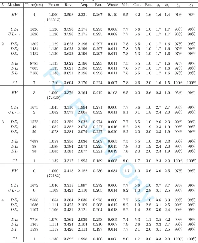
For each scenario, each solution method is applied over a rolling horizon of T = 30 periods. Table 2 summarizes the results. The first column denotes the maximum shelf live L_{∈ {2, 3, 4}. The} sec-ond column indicates the solution methods applied to determine delivery quantities and routes for each scenario, namely: the expected value method (EV ), up-to-level with daily deliver-ies (U L1), deliver-up-to-level with large delivery quantities to satisfy T SL for λ = L− 1 periods

(U LL−1), decomposition without costs-to-serve (DE0), decomposition with distance-based

costs-to-serve (DEd), decomposition with route-based costs-to-serve (DEr), decomposition-integration

without costs-to-serve (DI0), decomposition-integration with distance-based costs-to-serve (DId),

decomposition-integration with route-based costs-to-serve (DIr), and the full information method

(F I).

Column 3 displays the average computation times over 30 scenarios for each instance. When L = 2, most of the computation time is spent in solving the VRPs, in that all N = 40 stores are served in every period when applying U Lλ, DE, or DI. When L = 4, however, most of the computation time

is devoted to solving the expensive SDP relations (7). In the latter case, solving the VRPs takes almost no time because the average number of stores served in each period is around 15.

The next columns report, respectively, average values over 30 scenarios of the profit, revenue, acquisition cost, routing cost, waste cost, average number of vehicles per period, average number of stores per route, average time between two consecutive visits to stores, freshness on shelf, freshness from customers’ perspective, service level based on the number of stock-outs, and service level based on the filling rate.

In order to increase the readability of the table, the values in Columns 4–8 are normalized with respect to the profit obtained by EV for each shelf life (the absolute value of the profit obtained by

EV is shown between parentheses). For U Lλ, we obtained the highest profit by setting λ = L− 1.

For F I, we obtained the highest profit by setting λ = 2 (resp., 3, 3) for L = 2 (resp., 3, 4). 3 4 5 6 7 8 9 10 11 12 13 14 15 16 17 18 19 20 21 22 23 24 25 26 27 28 29 30 31 32 33 34 35 36 37 38 39 40 41 42 43 44 45 46 47 48 49 50 51 52 53 54 55 56 57 58 59