Characterization of time-varying regimes in remote sensing time series: application to the forecasting of satellite-derived suspended matter concentrations

HAL Id: hal-01188636

https://hal.archives-ouvertes.fr/hal-01188636

HAL is a multi-disciplinary open access archive for the deposit and dissemination of sci-entific research documents, whether they are pub-lished or not. The documents may come from teaching and research institutions in France or abroad, or from public or private research centers.

L’archive ouverte pluridisciplinaire HAL, est destinée au dépôt et à la diffusion de documents scientifiques de niveau recherche, publiés ou non, émanant des établissements d’enseignement et de recherche français ou étrangers, des laboratoires publics ou privés.

Characterization of time-varying regimes in remote

sensing time series: application to the forecasting of

satellite-derived suspended matter concentrations

Bertrand Saulquin, Ronan Fablet, Pierre Ailliot, Grégoire Mercier, David

Doxaran, Antoine Mangin, Odile Fanton d’Andon

To cite this version:

Bertrand Saulquin, Ronan Fablet, Pierre Ailliot, Grégoire Mercier, David Doxaran, et al.. Char-acterization of time-varying regimes in remote sensing time series: application to the forecasting of satellite-derived suspended matter concentrations. IEEE Journal of Selected Topics in Applied Earth Observations and Remote Sensing, IEEE, 2014, 8 (1), pp.406 - 417. �10.1109/JSTARS.2014.2360239�. �hal-01188636�

Characterization of geophysical regimes in remote sensing

1

time series: application to the forecasting of satellite-derived

2

suspended matter concentrations.

3

Bertrand Saulquin (1, 2), Ronan Fablet (2, 3), Pierre Ailliot (3), Grégoire Mercier (2, 3), David 4

Doxaran (4), Antoine Mangin (2), Odile Fanton d'Andon (2). 5

(1) ACRI-ST, Sophia-Antipolis, 260 route du Pin Montard, BP 234 6

06904 Sophia-Antipolis, France 7

(2) Institut Mines-Telecom, Télécom Bretagne; UMR CNRS 3192 Lab-STICC, Technopôle 8

Brest Iroise CS 83818, 29238 Brest, France 9

(3) Université Européenne de Bretagne, 35000 Rennes, France 10

(4) CNRS, Université Pierre et Marie Curie-Paris 6, UMR 7093, Laboratoire d’Océanographie 11

de Villefranche/Mer, 06230 Villefranche-sur-Mer, France 12

Corresponding author: bertrand.saulquin@acri-st.fr 13 Submission date: 19/05/2014 14

Abstract(

Satellite data, with their spatial and temporal coverage, are particularly well suited for the 17

analysis and characterization of space-time-varying relationships between geophysical processes. In 18

this study, we investigate the forecasting of a geophysical variable using both satellite observations 19

and model outputs. The studied latent-regime models aim here at identifying time-varying regime 20

Characterization of time-varying regimes in remote sensing time

series: application to the forecasting of satellite-derived suspended

matter concentrations

shifts within a dataset which is a key of interest for geophysical processes driven by the seasonal 21

variability. As a specific example, we study the daily concentration from 2007 to 2009 of mineral 22

suspended particulate matters estimated from the satellite-derived MODIS, MERIS and SeaWiFS 23

dataset, in coastal waters adjacent to the Gironde River mouth (South West of France). We clearly 24

show that the forecast of the high resolution suspended particulate matter dataset using 25

environmental data (wave height, wind strength and direction, tides and river outflow) and a multi-26

regime model is significantly improved compared with a classical multi-regression and a Support 27

Vector Regression model. Each regime is here characterized by a regression function and a 28

covariance structure. 29

From an analytical point of view, we compare the results obtained with four models: 30

homogeneous and non-homogeneous Markov-switching models, with and without an 31

autoregressive term, i.e. the suspended matter concentration observed the day before. Inclusion of 32

an autoregressive term is motivated by the strong natural autocorrelation level depicted by 33

geophysical time series, but, one may avoid this term if, for example, the observations are no more 34

available during specific conditions or periods. With the evaluated models, best results are obtained 35

with a mixture of 3 regimes for both autoregressive and non-autoregressive models. Prediction 36

performance at day+1, using the non-autoregressive models and a validation dataset, reached 80% 37

of the observed variance, compared to 32% for a standard single-regime (regression) analysis, and 38

40 % for a Support Vector Regression. Inclusion of an autoregressive term increases results to 93% 39

of explained variance for the mixture model compared to 80% without autoregressive term and 85% 40

using a Support Vector Regression. These results stress the potential of the identification of 41

geophysical regimes to improve the forecasting, or the inversion, of a high resolution geophysical 42

variable using both observations and model outputs. We also show that for short periods of lack of 43

observations (less than 15 days), estimations using the autoregressive term are better than without. 44

In this case the autoregressive term and the transition probabilities between regimes are estimated 45

using available model outputs. 46

Index term: 1) Satellite-derived suspended matter time series analysis. 2) Statistical forecasting. 3) 47

Regime-switching latent regression models. 4) Joint analysis of satellite-derived products and 48

operational model outputs. 5) Gironde river plume. 49

1 Introduction(

50 51

The forecasting of a geophysical variable using statistical models is an alternative to model-52

based approaches which typically involve complex simulation and/or assimilation [1, 2]. For 53

instance, coupled hydrodynamic and sediment transport models can be used to estimate the 54

concentration of suspended particulate matters within the water column [3] while statistical 55

approaches may use available satellite and model data to predict the same variable [4]. Many 56

statistical approaches have been proposed and evaluated to forecast or infer a studied variable from 57

predictors. Among them, linear multivariate regression [5] and non-linear (polynomial) multivariate 58

regression [6] are the most known. Numerous specific models dedicated to time-series analysis such 59

as AutoRegressive Moving Average (ARMA) and AutoRegressive Integrated Moving Average 60

(ARIMA) models [7] have also been developed initially to address financial time series. These 61

latest, which aim at studying the behavior of a time series without considering forcing factors, have 62

also been applied to geophysical time series [8]. Non-linear regressions, based on supervised 63

learning strategies, such as Neural Networks [9] and Support Vector Regressions (SVR) [10] may 64

provide relevant alternatives to estimate a variable from predictors. In the context of geophysical 65

studies, they may nevertheless suffer from two major drawbacks. First, though relevant regression 66

performances may be reported, these models are not physically interpretable and may be very 67

sensitive to the training dataset. Second, multi-regime dynamics, often exhibited by geophysical 68

processes driven by the seasonality [11], cannot be addressed by non-linear models, contrary to 69

latent-regime models as demonstrated in our study. 70

We propose here to characterize time-varying relationships between a variable and its forcing 71

parameters using latent-regime models, and hence optimize forecasting results. As an illustration, 72

we address the concentration of inorganic suspended particle matters (SPIM), estimated from 73

satellite data using a regional algorithm [12, 13], and observed in the mouth of the Gironde estuary. 74

In this area, sediments are mainly exported from the Gironde estuary [13, 14] and SPIM 75

concentration clearly depends on the local physical forcing: swell, tide, wind and river discharge. A 76

minimum of energy has to be brought by waves and tides to re-suspend cohesive sediments 77

accumulated at the bottom. Conversely, when sediments have been re-suspended in the water 78

column by wave influence, their settling velocity depends on their size and density [15] and 79

physico-chemical properties [16]. This example stresses that the relationships between the studied 80

variable (SPIM) and the causing factors evolve in space and time and potentially requires advanced 81

statistical methods to identify the underlying geophysical regimes. 82

From a methodological point of view, “latent regime regressions” also referred as “clusterwise 83

regressions” [17, 18] are particularly appealing to identify such non-linear and multi-regime 84

patterns within a dataset. Each regime is associated with a linear regression and a non-linear 85

relationship is thus estimated as a sum of linear contributions. Regarding the temporal dynamics of 86

these regimes, we here consider Markovian processes [19], which state the transitions in time 87

between two regimes. The standard Hidden Markov Model (HMM) and Non-Homogeneous 88

Markov Model (NHMM) are evaluated [19]. The inclusion of an autoregressive term (HMM-AR) 89

and (NHMM-AR) is also discussed. This aspect is motivated on the one hand by the strong 90

autocorrelation level depicted by geophysical time series [20]. When the observation at t-1 is 91

available, it is obvious, considering the strong natural autocorrelation of geophysical data that the 92

forecast at time t should take into account the observation at time t-1. Conversely, for specific 93

applications, or if the observations are not available during long periods (such as winter storms, or 94

after a sensor failure), one may need to estimate the variable without using the observations of the 95

previous days. We discuss here the choice between autoregressive or not autoregressive models for 96

long lack of observation period using forecasting results from t+1 to t+15. 97

Model parameter estimation is carried out from a dataset composed of 5862 time series of 1096 98

points in the mouth of the Gironde estuary in the [3°W-1°E ; 45-46.5°N] area during the period 99

2007-2009. Validation is performed on the same area for using the data for the year 2010. We used 100

EOFs to reduce the dimension of the space-time observations. This is a usual approach in spatio-101

temporal statistics [21, 22] although alternatives may be considered such as linear discriminant 102

analysis [23], and, we could also introduce a latent variable to describe the regime at each location 103

and interact with the regimes at other locations. Nevertheless, such models are known to be very 104

difficult to fit on the data and remain a research challenge for statisticians. We infer our mixture 105

model using the expansion coefficients of the first four modes of the EOF which explain 99% of the 106

total variance. The variables used as predictors for the SPIM expansion coefficients (EC) are the 107

wave height issued from a numerical model [24], the wind fields optimally interpolated from 108

satellite observations [25], the tide coefficient [26] and the Gironde fresh water discharge (sum of 109

the Garonne and Dordogne Rivers contributions). 110

2 Methods(

2.1 Markov(switching(forecast(models(

We address here the study of a two dimensional scalar geophysical time series Y. In a hidden 114

Markov model framework (HMM; [19]), one states two different processes, the observed process Y 115

and a hidden process Z. The observed process (here the turbidity) is assumed to be temporally 116

dependent of the hidden process. The hidden process Zt is modeled as a first order Markov chain

117

[19]. At a given time t, the hidden variable Zt = k is a discrete value which states the regime

characterized by a latent [17] regression model with coefficient Bk between the variable Yt and the

119

predictor Xt. At time t, knowing regime variable Zt, the observed variable Yt is modeled as:

120

(𝑌𝑡"|"𝑍𝑡=𝑘)="𝑋𝑡𝐵𝑘" (1) 121

where 𝑋𝑡𝐵𝑘 is the regression function, which predicts variable Yt from some predictors Xt for

122

regime Zt = k.

123

Figure 1 shows a graphical representation of the conditional dependencies involved in the 124

model, in the form of the general Directed Acyclic Diagram (DAG). It illustrates the interactions 125

between the variable Yt,, the predictors Xt, the hidden regime Zt and the covariate St which acts on

126

regime switching. Xt may contain lagged values of Yt (referred as autoregressive terms) and/or

127

exogenous covariates such as wind or wave height. Figure 1 defines a general family of model 128

which encompasses the most usual ones with regime switching. When no covariate is considered 129

i.e., Zt only depends Zt-1, and, Yt, only depends on (Yt,-s ..Yt,-1) and Zt, we retrieve the usual Markov

130

switching autoregressive (MS-AR). If we further assume that s=0 (without autoregressive 131

component where Yt, only depends on Zt) then we obtain the Hidden Markov Models (HMMs).

132

When Zt does not dependent on Zt-1, and the dependence on St is parameterized using indicator

133

functions, we obtain the threshold autoregressive (TAR) model which is the other important family 134

with regime switches in the literature. HMMs, MS-AR and TAR have been used in many fields of 135

applications including geosciences [27]. 136

137

Figure 1: Graphical representation of the various Markov-Switching Models considered in this 138

work: the arrows state the conditional dependencies between the random processes in play, namely 139

hidden regime process Z, observed process Y, prediction process X and regime change covariate 140

process S. 141

In the following equations (2 to 14), Xt and St are known, as they are either observations or

142

numerical model outputs. Given (1) the conditional likelihood of the observation Yt given

143

predictors Xt and regime Zt is expressed as [17]:

144

PYtXt,Zt=k~N(XtBk,σk) (2)

145

where N represents the Gaussian probability density function with mean XtBk and covariance 146

σk. Hence, given predictors up to time t we can predict process Y from its expectation conditionally

147

to process X: 148

𝑌𝑡=𝐸"𝑌𝑡𝑋𝑡=𝑘=1𝐾𝑃𝑍𝑡=𝑘𝑋𝑡"."EYtXt,Zt=k=𝑘=1𝐾𝑃𝑍𝑡=𝑘𝑋𝑡"."XtBk"" (3)

149

where K is the number of regimes. 𝑃𝑍𝑡=𝑘𝑋𝑡=𝜋𝑡𝑘0 is the posterior probability that the 150

dynamical regime Z at time t is of type k [17]. 151

3 Markov=switching(priors(

152 153

Stating hidden regime process Z as a first-order Markovian process amounts to modeling the 154

transition between successive regimes at time t and time t-1. In the simplest case, one assumes 155

homogeneous transitions, i.e. time-independent and context-independent transitions, and the 156

Markovian process is fully characterized by its transition matrix P(Zt =k | Zt-1 =l) for possible pairs

157

of successive regimes (k, l). In the HMM setting the conditional distribution of Zt, given the past

158

values Ys and Zs for s<t, is assumed to depend only on Zt-1 (Fig. 1):

159

𝜋𝑡𝑘0=𝑃𝑍𝑡=𝑘0𝑌0..𝑌t)=0𝑙=1𝐾𝑃𝑌𝑡0𝑍𝑡0=𝑘.𝑃(𝑍𝑡0=𝑘𝑍𝑡−10=𝑙.𝑃𝑍𝑡−1=𝑙0𝑌0..𝑌t−1) (4) 160

A NHMM extends this idea by allowing the transition matrix between the hidden states to 161

depend on a set of observed covariates St. Hughes and Guttorp [28, 29] highlighted the added value

162

of the NHMM to characterize the links between the large-scale atmospheric measures and the 163

small-scale spatially discontinuous precipitation field. In the NHMM settings, the transition matrix 164

between states 𝑃(𝑍𝑡"=𝑘𝑍𝑡−1"=𝑙 in (3) is now time-dependent and conditioned by the covariates St:

165 𝜋𝑡𝑘0=𝑃𝑍𝑡=𝑘0𝑌0,..,𝑌t,00St)= 166 𝑙=1𝐾𝑃𝑌𝑡0""𝑍𝑡0=𝑘,.𝑃(𝑍𝑡0=𝑘𝑍𝑡−1=𝑙,"St.𝑃𝑍𝑡−1=𝑙"0𝑌0"..𝑌t−1) (5) 167 with: 168

𝑃(𝑍𝑡=𝑘0𝑍𝑡−10=𝑙,00St=𝑃St00𝑍𝑡0,=𝑘,"""𝑍𝑡−10=𝑙0.00𝑃𝑍𝑡0=𝑘𝑍𝑡−10=𝑙000/0

169

𝑘,𝑙𝑃St00𝑍𝑡=𝑘0,0"𝑍𝑡−10=𝑙0.00𝑃𝑍𝑡0=𝑘𝑍𝑡−10=𝑙 (6)

170

The non-homogeneous transition between states is derived from the likelihood of the covariate 171

St given the state transition (Zt, Zt+1). We suppose that the probability density function of the

172

covariates during this change of state follows a normal distribution: 173

PSt0""Zt0=k,00Zt−10=l=Nµl,0k,0Σl,0k (7) 174

Where N is a multivariate normal distribution with n means 𝜃𝑠=µl,0 k,0 Σl,0 k, µ is here of 175

dimension n, the number of covariates used to estimate the transitions. For a ‘standard’ multivariate 176

gaussian distribution Σl,k is a covariance matrix. In the present application, and to reduce the

177

number of parameters to be estimated, we consider that the predictors are uncorrelated (null 178

covariance) and their relative influence is identical (same variance), i.e. Σl,k is a multiple of the

179 identity matrix. 180 181

3.1 Estimation(of(the(model(parameters((

The considered models involve two categories of parameters: those of the observation model, θk,

184

namely regression coefficient Bk and standard deviation σk for each regime (Eq. 2) and those of the

185

Markov-swtiching prior, namely θs (Eq. 5). Given observed Y and X series, we proceed to the

186

estimation of model parameters according to a classical maximum likelihood (ML) criterion using 187

an iterative Expectation Maximisation (EM) procedure [30] expressed here without covariates: 188

𝐿𝜃="𝑡PYtY0.."Yt−1,0θ (8) 189

where θ = {θs, θk} is the set of parameters to be estimated. For a given initialization for the

190

parameters the EM procedure iterates estimation steps (E-step) of the posterior regime likelihood 191

𝜋𝑡𝑘"with the given modes and the maximisation step (M-step) for the update of the parameters given

192

these posteriors. The algorithm iterates until convergence between steps n and n+1, i.e. 193

|𝐿𝜃(𝑛)−𝐿𝜃(𝑛+1)|<10−3 . The posterior likelihood 𝜋𝑡𝑘" (Eq 3&4) of the latent regime Zt, is

194

estimated in the E-step using the classical forward-backward recursions [31, 32] given series X and 195

Y and current parameter estimate θk(n), θs(n). The M-step re-estimates the parameters θk(n+1), θs(k+1).

196

For this, it is often possible to break the optimization problem into several lower dimensional 197

optimization problems which are much quicker to solve [32]. More precisely, for all the models 198

considered in this paper, it is possible to separate the parameters related to the evolution of the 199

hidden Markov chain θs, and the parameters related to the evolution of the observed process in each

200 regime θk: 201 θ=0𝑎𝑟𝑔𝑚𝑎𝑥𝜃𝑠00𝑡log⁡(𝑃(𝑍𝑡=𝑘0𝑍𝑡−10=𝑙,00St,θ𝑠(n))𝑃𝑍𝑡=𝑘,𝑍𝑡−10=𝑙"Y0.."YT,0St,0θ(n)00 (9) 202 θ𝑘""𝐵𝑘0(n+1)=𝑎𝑟𝑔𝑚𝑖𝑛𝐵𝑘𝑡𝑃𝑍𝑡=𝑘Y0.."YT,θ(n))0(𝑌𝑡−𝐵𝑘𝑋𝑡2)00000000000000000000000(10)0𝜎𝑘0(n+1)=𝑡𝑃𝑍𝑡=𝑘Y0.." 203 YT,θ(n))00(𝑌𝑡−𝐵𝑘𝑋𝑡2)0000000000000000000000000000000000000000000(11) 204 205

3.2 (Forecasting(application(

The considered multi-regime regression models are applied to the short-term forecasting of 208

series Y. More precisely, at a given time t, we aim at predicting variable Y at time t+dt. We 209

typically assume that prediction variables X and covariates S, typically numerical simulations, are 210

available up to time t+dt whereas the variable Y is only known up to time t. is estimated using 211

X0..t+dt and S0.. +dt (for inhomogeneous transitions). Thus, Y𝑡+dt is given by the conditional

expectation of variable Yt+dt given observations series up to time t and predictor series up to time t+ 213 dt: 214 (12) 215

For HMM and NHMM it resorts to: 216

(13) 217

For autoregressive models HMM-AR and NHMM-AR, i.e. Xt +dt contains Yt +dt -1 which is not

218

available, is estimated using Yt .. , Xt .. Xt+dt-1 and . Estimated Y𝑡+dt resorts to:

219

(14) 220

It might be noted that these predictions actually account for the uncertainties in the 221

determination of the underlying regimes. Contrary to deterministic methods, confidence interval 222

and uncertainties on Y𝑡+dt can be derived [33] which is a key issue for modeling considerations.

223

224

3.3 Model(performance(estimation((

225 226

A key issue in practice, which has received lots of attention in the last few years, is the problem 227

of model selection which aims at finding the ”optimal” number of predictors and covariates [31]. 228

Hereafter, we have chosen to use both the Bayes Information Criterion (BIC) and the explained 229

variance (EVAR) as a first guides. BIC index generally permits to select parsimonious models 230

which fit the data well [34]. It is defined as: 231

BIC = − 2 log*(L) + p*log(S) (15) 232

Where L is the likelihood of the data, p is the number of parameters and S is the number of 233

observations. The likelihood which is an output of the backward-forward recursions performed in 234

the E-step. We also use the classical explained variance, EVAR, to characterize the model 235

relevance: 236

0EVAR=1.−var0Y𝑡+1−Y𝑡+10/0var(Y𝑡+1) (16) 237

BIC and EVAR are partially linked [34]. BIC tends to penalize complex models whereas 238

explained variance criterion only qualifies the result and may lead to the over-parameterization of a 239

model that typically lead to errors when other dataset are tested using the same parameterization. 240

Therefore we consider both BIC and EVAR to assess the model performance. 241

The choice of the predictors and the covariates is performed here as follows. We first select as 242

predictors the variable showing a significant correlation with the studied variable. Given these 243

predictor datasets, we tested all the possible configurations and chose the predictors which provide 244

the lower BIC on the training dataset and the greatest EVAR using the training (EVAR_train) and 245

the validation dataset (EVAR_valid). 246 247

4 The(data(

4.1 The(studied(variable(

Non-algal SPM concentrations (SPIM) are estimated using an analytical algorithm [12] defined 252

as the difference between total SPM and phytoplankton biomass, the latter derived from Chl-a. It 253

incorporates mainly mineral SPM and smaller amounts of organic SPM not related to living 254

phytoplankton. This method to derive non-algal SPM from remote-sensing reflectance is based on 255

the inversion of a simplified equation of radiative transfer, assuming that chlorophyll concentration 256

is known. This merged dataset consists of fields of non-algal surface SPM concentrations, derived 257

from the Sea-viewing Wide Field-of-view Sensor (SeaWiFS), the Moderate Resolution Imaging 258

Spectroradiometer (MODIS) and the Medium Resolution Imaging Spectrometer (MERIS) sensors, 259

provided by the Ocean Colour TAC (Thematic Application Facility) of MyOcean, and interpolated 260

with a kriging method [35] for the period 2007–2009 over the Gironde mouth river from 3°W-1°E ; 261

45-46.5°N. Finally 5682 continuous time series of 1096 days compose our initial dataset of mineral 262

suspended matters concentration. 263

We first account for the space-time variability of the dataset, previously detrended and centered 264

for each time series [37] using a EOF decomposition [21], expressed here using the matrix form: 265

Cov(SPIM)=UVUt (17)

266

where U is a here 5682*5682 matrix containing the spatial modes (Eigenvectors) of the 267

covariance decomposition (ordered by percentage of explained variance). Associated with each 268

spatial mode k, its expansion coefficient (also referred in the literature as principal component) is 269

the time evolution of the kth _mode:

270

EC_SPIM k,t = SPIM t * Uk (18)

271

Figure 2 shows the four first spatial modes of the EOF decomposition. Figure 3 depicts the four 272

associated time series EC_SPIMi=1,4. The first mode (Fig.2a) comprises 85% of the total variance. It

273

clearly addresses the seasonal cycle as shown in Fig. 3a where the switch between winter (high 274

values of EC_SPIM1 correspond here to high values of SPIM observed in winter) and summer

275

periods is clearly visible. The variability around the seasonal mean is captured by the other modes 276

(Fig.2 c-e & Fig 3 c-e). Mode 2 refers to the inter-annual and the intra-seasonal variability in the 277

shoreward gradient and represents 7% of the total variance. Mode 3 addresses some North-South 278

gradients and represents 4% of the total variance and mode 4 is clearly influenced by the Gironde 279

river (Fig. 2d), which brings sediments during water outflow, and represent 3% of the variance. By 280

construction, EOF decomposition imposes the orthogonality [21] of the spatial modes (Fig. 2). 281

Figure 2: spatial modes of the EOF decomposition of the SPIM observed from satellite from 282

2007-2009 in the Gironde mouth river. From left to right and top to bottom the first four EOF 283

modes account respectively for 85, 7, 4 and 3% of the total variance. 284

b a

Figure 3: EOF decomposition of the SPIM observed from satellite from 2007-2009 in the 285

Gironde mouth river: from left to right and top to bottom, the expansion coefficients (EC_SPIM1-4)

286

associated with the first four EOF modes depicted in Fig. 2, i.e. the time evolution of the spatial 287

modes. The reconstruction of the SPIM variable from the estimated ECs is performed as: 288

SPIM𝑡0=0𝑘EC_SPIM0.0𝑈𝑘 (19)

289

The total explained variance using the 4 first modes is shown Fig. 4. On average, the explained 290

variance represents 99 % of the total variability on the areas with some local minima of 60% 291

observed at the very near-shore and the Southwestern part of the area. 292

a b

293

Figure 4: Variance explained by the four first modes of the EOF decomposition of the 294 suspended matters. 295 296

4.2 Predictors(and(covariates(

The predictors X are the variables used in the estimation of Y and Z any time (Eq. 13 & 14). We 299

used here wave height (WH) daily means of the Wave Watch 3 model (WW3; [24, 36]) provided by 300

the IOWAGA and PREVIMER programs, Western and Northern winds interpolated from 301

QuickSCAT and ASCAT observations in conjunction with ECMWF forecasting [25], provided by 302

Ifremer, tide index (SHOM, 2000) at Bordeaux and the flow measurement of river la Gironde. 303

Similarly to the SPIM data, all the data were log transformed. For the wind data which is signed, the 304

transformed log variable was signed negatively a posteriori to the log transformation. The WH first 305

mode of the EOF decomposition explained 98 % of the total variance, 93% for the Northern wind 306

(WND1), and 96% for the Western wind (WND2). Covariates are the normalized predictors used in 307

the estimation but considered at t-2. This lag has been estimated as the optimal time-lag using BIC 308

and EVAR results on the training dataset. 309

310

5 Results(

311 312

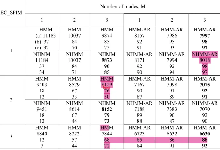
We summarize in Table 1 the prediction performance for the first four ECs of the SPIM issued 313

from four models: HMM, NHMM, HMM-AR, and NHMM-AR. The number of considered modes 314

for the mixture varies from 1 to 3. The one-mode models refer to a simple multivariate regression 315

analysis. For each configuration we provide the BIC and EVAR_train on the training dataset 316

(2007-2009) and EVAR_valid on the validation dataset (2010). Note that the selection of the 317

predictors and resulting covariates is achieved as a prior step as described in Section 2.6. The first 318

mode of the EOF decomposition explains 85% of the total variance. EC_WH1 and EC_WND21

319

(respectively the expansion coefficient of the first EOF of the Western winds) are identified as 320

being the relevant predictors. This mode captures the mean seasonal variability of the SPIM, which 321

is mainly driven by WH and the North Atlantic storms and at a second order by the Western winds. 322

For EC_SPIM1, when no autocorrelation term is used, the best fit is obtained for a 3-regime

323

NHMM model (BIC= 9873, EVAR_train=90% and EVAR_valid=85%). When a first order 324

autocorrelation term is added, the best fit is issued from a 3-regime HMM-AR model: BIC= 7997, 325

EVAR_train = 98% and EVAR_valid = 97%. The lag-1 autocorrelation value is 0.85 for 326

EC_SPIM1, and therefore the weight given Yt-1 is important compared to the other covariates,

327

EC_WH1 and EC_WND21. This stresses the fact that when available first autoregressive term

328

should be included to enhance the performances 329

pas clair Text

The second mode of the EOF decomposition of the SPIM variability explains 7% of the total 330

variance. The selected predictors are the first mode of the Western wind, the tide, and the river 331

flow. The variability captured by EC_SPIM2 relates to the local Westward wind, which is not

332

captured by the WH model, and the very coastal variability introduced by the tide and the river 333

outflow. For the non-AR models the selected model was the three-regime NHMM. It is interesting 334

to note in this case that EVAR_valid increased from 50 to 73% between the HMM and the NHMM, 335

highlighting the contribution of the non-homogeneous transition model. By contrast, the HMM-AR 336

performed slightly better than the NHMM-AR. 337

Table 1: Model performance for each EOF mode of the SPIM variability. For each 338

configuration we report the BIC (a) and the explained variance (EVAR_train, b) for the training 339

dataset (2007-2009), and the explained variance (EVAR_valid, c) for the validation dataset (2010). 340

In bold are highlighted for each EC the selected configurations (see § 5.2). 341 Number of modes, M EC_SPIM 1 2 3 1 2 3 HMM (a) 11183 (b) 37 (c) 32 HMM 10037 84 70 HMM 9874 85 75 HMM-AR 8157 92 91 HMM-AR 7986 95 93 HMM-AR 7997 98 97 1 NHMM 11184 37 34 NHMM 10037 84 71 NHMM 9873 90 85 NHMM-AR 8171 92 90 NHMM-AR 7994 92 94 NHMM-AR 8018 98 97 HMM 9403 18 12 HMM 8579 67 33 HMM 8129 76 50 HMM-AR 7167 90 87 HMM-AR 7098 91 89 HMM-AR 7075 92 91 2 NHMM 9451 18 12 NHMM 8614 67 44 NHMM 8152 79 73 NHMM-AR 7188 89 88 NHMM-AR 7383 90 87 NHMM-AR 7070 92 90 3 HMM 8840 12 7 HMM 8222 57 44 HMM 7844 68 72 HMM-AR 6723 85 84 HMM-AR 6632 86 91 HMM-AR 6630 88 92 niveau de contribution des variables complémentaires

NHMM 8866 11 16 NHMM 8246 59 45 NHMM 7862 75 76 NHMM-AR 6745 88 86 NHMM-AR 6673 88 91 NHMM-AR 6703 88 92 HMM 8248 18 28 HMM 7596 60 63 HMM 7285 71 72 HMM -AR 6398 85 86 HMM -AR 6416 85 86 HMM -AR 6313 86 86 4 NHMM 8276 18 28 NHMM 7628 62 59 NHMM 7267 70 75 NHMM-AR 6426 85 83 NHMM-AR 6445 85 83 NHMM-AR 6357 86 85 342

The third mode of the EOF decomposition of the SPIM variability explains 4% of the total 343

variance. It captures some inter-annual and intra-seasonal variability of the latitudinal gradient of 344

the SPIM. The selected predictors are EC_WH1, EC_WND11 (Northern)and the tide. Once again,

345

three-regime NHMM and HMM-AR provide the best results. 346

Regarding the fourth mode of the EOF decomposition of the SPIM variability, which accounts 347

3% of the total variance, EC_WH1, EC_WND21, the tide and the river flow are selected as

348

contributive predictors. We reconstruct 75 % of EC_SPIM3 variance of the validation dataset using

349

a three-regime NHMM and 86% using a three-regime HMM-AR. We note that globally, the three 350

indices (BIC, EVAR_train and EVAR_valid) tend to select the same models. 351

352

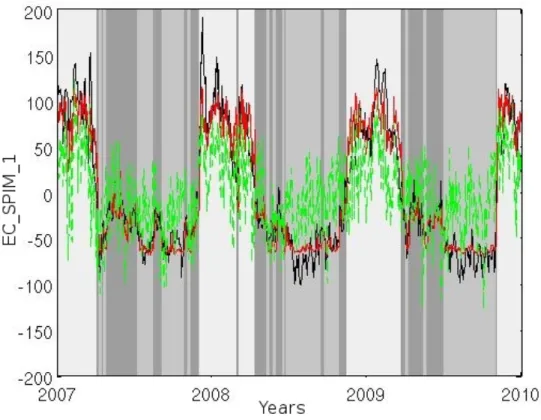
5.1 Example(with(the(estimation(of(EC_SPIM

(

353 354

We report in Figure 5 the temporal evolution of the three regimes of the NHMM for EC_SPIM1.

355

In table 2 are shown the corresponding coefficients for each predictor and the intercept. The first 356

regime (light grey), characterized by high SPIM levels (intercept of 65), is referred as a ‘winter 357

regime’. The’ winter regime’ also strongly relates to the wave height (WH regression coefficient of 358

0.6). Dark grey periods (regime 3) are identified as a ‘transition regime’, and medium grey (regime 359

2) identified as the ‘summer regime’. For regimes 2 and 3, the coefficients for WH decrease 360

respectively to 0.12 and 0.09. In summer the energy brought by waves is not sufficient enough to 361

re-suspend massively the sediments. It might be noticed that for all regimes the wind conditions 362

show a small but significant effect on EC_SPIM1. When an autocorrelation term is added

(HMM-363

AR, table 2), the AR(1) coefficient value is 0.86 for the regime 1 (winter), and 0.9 for regime 2 and 364

3 which underlies the natural higher autocorrelation level of SPIM when the concentration is low. 365

Figure 4 compares the prediction of EC_ SPIM1 using a single multivariate regression (green)

366

and the proposed multi-regime NHMM. In this case the explained variance value (Table 1) is of 367

37% for the multivariate regression model compared to 85% for the three-regime NHMM. 368

369

Figure 5: Estimation of the EC_SPIM1 (in black) using EC_WH1, EC_WND21 anda single

370

regression (green) and a 3 regime NHMM (red). The nuances of grey in the background highlight 371

the temporal distribution of the regimes. 372

Table 2: Estimated regression parameters for each of the three regimes of the NHMM and the 374

HMM-AR for the first mode of the SPIM EOF decomposition: regression parameters involve an 375

intercept and the regression coefficients of the wave height and western wind velocity. 376

EC_WH1 EC_WND2 Intercept

NHMM (1, winter) 0.6037 (2, summer ) 0.0910 (3, transition) 0.1210 -0.0632 0.0006 0.0100 65.0672 -61.6442 -24.6578

EC_WH1 EC_ WND2 Intercept AR(1)

HMM-AR (1) 0.2383 (2) -0.0050 (3) 0.0354 -0.0033 0.0168 0.0035 4.4694 -3.9531 0.6079 0.86 0.90 0.90 377

Figure 6 illustrates the non-homogeneous transition used in the NHMM between the ‘transition’ 378

(Zt=3) and ‘winter’ (Zt =1) regimes. The probability of switching from regime 3 to 1 increases with

379

wave height covariate WH1 with a probability of switching close to zero when WH1 is negative and

380

a probability close to one for large WH1 values.

381

382

Figure 6: Non-homogeneous transition between ‘transition regime’ (Zt=3) (light grey Fig. 5) 383

and ‘winter regime’ (Zt=1) (light grey Fig. 5) as a function of the wave height covariate WH1.

384

variance expliqué par chaque terme

5.2 Forcasting(of(the((SPIM((on(the(2010(validation(dataset(

385 386

We forecast SPIM fields from the reconstructed ECs and the selected models (Table 1 & Eq. 387

19). Figure 7a&7b compare EVAR_valid of the initial field (SPIM) using the three-regime NHMM 388

and NHMM-AR models selected in Table 1 for their results. On average we were able to predict at 389

t+1 80% of the variance using the NHMM (Fig. 7a) and 90% using the NHMM-AR. The spatial 390

distribution of the error is not homogeneous. Fig. 7a shows that EVAR_valid value is of 90% in the 391

Northern part with nevertheless poorer results in the South. Fig. 7b shows that the AR1 component

392

of the model increases EVAR for the whole area. 393

We also considsr the results of a standard multi-regression analysis. If only one regime is 394

considerer NHMM and HMM resort to a strandard multivariate regression and NHMM-AR and 395

HMM-AR to a strandard multivariate regression including an AR1 coefficient the transition

396

probabilities being equal to 1. Fig. 7c shows the obtained results with the standard multivariate 397

regression and Fig 7d the standard multivariate regression including an AR1. From Fig. 7c to 7a, the

398

gain in explained variance is in mean about 250% (from in mean 32% Fig. 7c to 80% Fig. 7a) while 399

for the AR models, the gain is about from 11% (from in mean 83% Fig. 7d to 93% Fig. 7b). 400

401

Figure 7: Explained variance for the 2010 validation dataset reconstructed using the selected 3-402

regime NHMM (a) and NHMM-AR (b), compared with the standard multivariate regression 403

without AR1 (c) and including an AR1 (d).

404

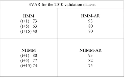
To consider the model forecast performances, we report the short-term forecast results at 405

different time steps (cf. Eq.13 & 14). For the HMM-AR and NHMM-AR (Eq. 14) is the estimated 406

value, the observation being not available (see § 3.2). Table 3 synthesizes the explained variance 407

statistics using 3 regimes and the four tested models for the forecasting at t+1, t+5 and t+15 and the 408

validation 2010 dataset (Eq. 19). 409

The long term forecasting results are globally better with the NHMM. At t+15 using the 410

NHMM we are able to forecast 74% of the variance for 2010, compared with 40% for the HMM. In

411

this case where the covariates and predictors (mode outputs for which the short term predictions are 412

assumed to be available) are used in the estimation of the regime transition probability . For 413

autoregressive models, at t+15, we were able to forecast 75% of the 2010 variance with the 414

NHMM-AR compared with 70% with the HMM-AR. For the NHMM-AR the covariates help in the 415

estimation of both and . At t+15 NHMM and NHMM-AR show equivalent results underlying the 416

maximal time-step to consider for the between these two models. 417

Table 3: Validation results on year 2010. Explained variance (Eq. 16) for the forecast at t+1, t+5 418

and t+15 of the 2010 validation dataset. 419

EVAR for the 2010 validation dataset HMM (t+1) 73 (t+5) 63 (t+15) 40 HMM-AR 93 80 70 NHMM (t+1) 80 (t+5) 77 (t+15) 74 NHMM-AR 93 82 75 420

SVR model was also evaluated to evaluate the performances of a non-linear model on the studied 421

dataset. To perform the comparison, we train the SVR model (http://www.csie.ntu.edu.tw) for each 422

EC using the same training dataset (2007-2009) and performed forecasting using the same 423

validation dataset (2010). We used the setting as following: model epsilon-SVR (s=3), linear or 424

polynomial kernel (t=0 or 1) and the same inputs (predictors, covariables) for each EC. Parameters 425

c and g [10] were optimised for each EC using the training dataset and the cross validation mode. 426

On the 2010 validation dataset, better forecast results reached 40% at t+1 of the EVAR (without 427

AR) and 85% with an AR coefficient. The results were significantly worse than those obtained 428

using the time-varying models for increasing time steps. The SVR can address non-linear 429

relationships, it cannot nevertheless deal with multi-regime processes. By contrast, the latent-regime 430

model addresses by nature multi-regime processes and can approximate non-linear relationships as 431

a series of linear models. 432

433

6 Discussion(

434 435

We investigated the relevance of four regime-switching latent regression models, namely 436

HMM, NHMM, HMM-AR and NHMM-AR to characterize time-varying linear relationships 437

between the high resolution inorganic suspended matter concentration (SPIM), estimated from 2007 438

to 2009 using MODIS, SeaWiFS and MERIS data in a coastal area, and its forcing conditions, i.e. 439

the wave height, the Northern and Western winds, the tides and the river flow. The estimated 440

regimes are then used to forecast the SPIM using the independent year 2010 dataset, from t+1 to 441

t+15. 442

An optimal number of three distinct geophysical regimes were needed to capture the different 443

dynamics and optimize forecasting performance. Autoregressive and non-homogeneous model 444

showed better performances. With the evaluated models and the 2010 validation dataset we were 445

able to forecast at t+1 80 % of the variance explained using a NHMM and 93 % using a NHMM-446

AR. In the latest case the strong natural autocorrelation of the studied signal is an important 447

predictor to consider. The explained variance on the prediction at +1 for a standard multivariate 448

regression was of 32% and 80% (with an AR1 term). Using a SVR we were able to forecast at t+1

449

respectively 40% and 85% (with an AR1) of the explained variance.

450

As illustrated for the first SPIM EOF component (Figure 5), the proposed multi-regime setting 451

allowed us to identify three seasonally varying relationships between the observed turbidity, the 452

wave height and the wind. We did not drive the model to account for seasonal regimes but we 453

identified three seasonally-discriminated regimes, with two leading factors: the mean SPIM level 454

(intercept) and the Western wave height. These regimes identified directly physical behaviors, here 455

the minimum of energy to be brought by the Western swell to re-suspend the sediments. This is 456

regarded as a key feature of the latent-regime model compared to other non-linear regression 457

models, such as Neural Networks [38] or SVR [10] which cannot address multi-regime 458

relationships and are hardly interpreted in general. Using our dataset the non-linear SVR was not 459

able to retrieve the regime changes. 460

Regarding long-term forecast performance, at t+15 best results obtained were of 74% of 461

explained variance for the NHMM and 75% for the NHMM-AR. For short period, typically from 1 462

to 15 days, when the observed Y is not available, NHMM-AR provided the best results. In this case 463

the predictors and covariates are used in the estimation of both and . At t+15 NHMM and NHMM-464

AR showed similar results underlying the maximal time-step to consider, when no observation of Y 465

is available, for the choice between these two models. 466

In the future, we will address the forecasting of the chlorophyll-a using satellite-derived 467

observations such as the photosynthetic available radiation, the temperature, the suspended matters 468

(as index of available nutrients) and light attenuation [39]. In this more complicated case, second 469

order relationships between the variable and its predictors have to be evaluated, the chlorophyll-a 470

dynamic being not anymore a passive result of the forcing conditions, as expected with the SPIM, 471

but having its proper characteristics depending on each phytoplankton specie. Extensions of the 472

considered latent regime setting to other inverse problems in satellite sensing data analysis are also 473

under investigation, such as latent regime inversion procedures for satellite-derived chlorophyll-a 474

concentration to account for different water types (turbid or not turbid) and/or the presence of 475

specific phytoplankton species. 476

7 Acknowledgements((

477 478

The authors thank Aldo Sottolichio from the Université of Bordeaux 1, for the provision of the 479

in-situ Gironde flow measurement, Pierre Tandeo for fruitful advises and the MCGS (Marine 480

Collaborative Ground Segment; http://www.mcgs.fr) project which aim at making the most of ESA 481

Sentinels satellites potential for users driven services based on high level products. MCGS 482

Tex t

addresses the need of the European Space Agency to build up data processing centers in 483

conjunction with the Copernicus Program for the provision of services to local and national, public 484

and private European institutions or entities involved in marine activities. The project is co-funded 485

by the French Government (Fonds Unique Inter-ministériel), local authorities of the Bretagne and 486

Provence-Alpes-Côte d'Azur regions and the European Regional Development Fund (ERDF), under 487

support of the French Space Agency (CNES). 488

8 References(

489 490

1 P. Lazure, V. Garnier, F. Dumas, C. Herry, M. Chifflet. “Development of a hydrodynamic model of

491

the Bay of Biscay”. Validation of hydrology. Continental Shelf Research, 29(8), 985-997, 2009.

492

2 L. Debreu, P. Marchesiello, P. Penven and G. Cambon, “Two-way nesting in split-explicit ocean

493

models: algorithms, implementation and validation”, Ocean Model., 49-50, 1-21, 2012.

494

3 A. Sottolichio, P. Le Hir, P. Castaing. “Modeling mechanisms for the turbidity maximum stability in

495

the Gironde estuary, France”, Coastal and Estuarine Fine Sediment Processes, pp 373-386, 2000.

496

4 A. Rivier, F. Gohin, P. Bryere, C. Petus, N. Guillou, G. Chapalain. “ Observed vs. predicted

497

variability in non-algal suspended particulate matter concentration in the English Channel in relation to tides

498

and waves”. Geomarine Letters, 32(2), 139-151, 2012.

499

5 C. Aitken, “On Least Squares and Linear Combinations of Observations”, Proceedings of the Royal

500

Society of Edinburgh, 55, 42–48, 1935.

501

6 William E. Wecker, Craig F. Ansley, The Signal Extraction Approach to Nonlinear Regression and

502

Spline Smoothing Journal of The American Statistical Association , 78(381):81-89, 1983.

503

7 Box, George; Jenkins, Gwilym, Time Series Analysis: forecasting and control, rev. ed., Oakland,

504

California: Holden-Day, 1976.

8 Tesfaye, Y. G., Meerschaert, M. M., and Anderson, P. L. Identification of periodic autoregressive

506

moving average models and their application to the modeling of river flows. Water Resources Research,

507

42(1), 2006

508

9 Some Neural Network applications in environmental sciences part I: forward and inverse problems in

509

geophysical remote measurements, V. Krasnopolsky and H. Schiller, Neural Networks, vol 16 (2003),

321-510

334.

511

10 Chih-Chung C., Chih-Jen L. LIBSVM: A library for support vector machines Transactions on

512

Intelligent Systems and Technology (TIST), 2011.

513

11 P. Ailliot, V. Monbet. “Markov-switching autoregressive models for wind time series”.

514

Environmental Modelling & Software, 30, 92-101, 2012.

515

12 F. Gohin, S. Loyer, M. Lunven, C. Labry, J.M. Froidefond, D . Delmas, M . Huret, A. Herbland,

516

“Satellite-derived parameters for biological modelling in coastal waters: illustration over the eastern

517

continental shelf of the Bay of Biscay”. Remote Sensing of Environnement 95(1), 29–46, 2005.

518

13 D. Doxaran, « Télédétection et modélisation numérique des flux sédimentaires dans l’estuaire de la

519

Gironde », PhD thesis, University Bordeaux 1, France, 326 pp, 2002.

520

14 D. Doxaran, J.M. Froidefond, P. Castaing and M. Babin. “Dynamics of the turbidity maximum zone

521

in a macrotidal estuary (the Gironde, France): Observations from field and MODIS satellite data”, Estuarine

522

Coastal and Shelf Science, 81, 321–332, 2009.

523

15 D.G. Bowers, C.E. Binding.”The optical properties of mineral suspended particles: a review and

524

synthesis”. Estuarine Coastal Shelf Science, 67(1/2), 219–230, 2006.

525

16 D. Eisma, P. Bernhard, G.C. Cadée, V. Ittekkot, J. Kalf, R. Laane, J.M. Martin, W.G. Mook, A. Van

526

Put, T. Schuhmacher, “Suspended matter particle size in some West-European estuaries; part II: a review on

527

floc formation and break up”, Netherlands Journal of Sea Research, 28(3), 215–220, 1991.

528

17 W. S. DeSarbo and W. L. Cron, “A maximum likelihood methodology for clusterwise linear 469

529

regression”, Journal of Classification, 5, 249–282, 1998

18 P. Tandeo, B. Chapron, S. Ba, E. Autret, R. Fablet, “Segmentation of Mesoscale Ocean Surface

531

Dynamics Using Satellite SST and SSH Observations Geoscience and Remote Sensing”, IEEE Transactions

532

on Volume, pp 1 – 9, 2013.

533

19 B.H. Juang, and L.R. Rabiner. “Hidden Markov models for speech recognition”, Technometrics, 33,

534

251-272, 1991.

535

20 C. Frankignoul and K. Hasselmann, “Stochastic climate models. Part II: Application to SST

536

anomalies and thermocline variability”. Tellus, 29, 289-305, 1977.

537

21 R.W. Preisendorfer, “Principal Component Analysis in Meteorology and Oceanography”, Elsevier,

538

New York,. pp 425, 1988.

539

22 Cressie NAC, Wikle CK. Statistics for Spatio-Temporal Data. Wiley; New York: 2011.

540

23 Abdi, H. "Discriminant correspondence analysis." In: N.J. Salkind (Ed.): Encyclopedia of

541

Measurement and Statistic. Thousand Oaks (CA): Sage. pp. 270–275, 2007.

542

24 F. Ardhuin, E. Rogers, A.V. Babanin, J. Filipot, R. Magne, A. Roland, A. van der Westhuysen, P.

543

Queffeulou, J.M. Lefevre, L. Aouf, F. Collard, “Semi-empirical dissipation source functions for ocean

544

waves. Part I: Definition, calibration, and validation”. Journal of Physical Oceanography, 40(9):1917–1941,

545

2010.

546

25 A. Bentamy, D. Croizé. Fillon, “Gridded Surface Wind Fields from

547

Metop/ASCAT Measurements”, International Journal of Remote Sensing, 33:

548

1729-1754, 2011.

549

26 Courants de marée et hauteurs d’eau. La Manche de Dunkerque à Brest. Service Hydrographique et

550

Océanographique de la Marine, Brest, Rapport 564-UJA, 2000

551

27 Tong, H. Non-linear time series, a dynamical systems approach. Oxford University Press, 1990.

552

28 J. P. Hughes and P. Guttorp. “A Class of Stochastic Models for Relating Synoptic Atmospheric

553

Patterns to Regional Hydrologic Phenomena”, Water Resources Research, 30, 1535-1546, 1994a.

29 J. P. Hughes and P. Guttorp, “Incorporating Spatial Dependence and Atmospheric Data in a Model

555

of Precipitation”. Journal Applied Meteorology, 33, 1503-1515, 1994b.

556

30 A.P. Dempster, N.M. Laird and D.B. Rubin, “Maximum likelihood from incomplete data via the EM

557

algorithm”, Journal of the Royal Statistical Society. Series B (Methodological), 39, 1–38, 1977.

558

31 F. Castino, R. Festa, and C.F. Ratto, “Stochastic modelling of wind velocities time series”, Journal of

559

Wind

560

32 W. Zucchini and P. Guttorp. “A hidden Markov model for space-time precipitation”, Water

561

Resources Research, 27, 1917–1923, 1991.

562

33 O. Cappe, E. Moulines, and T. Ryden. “Inference in hidden Markov models”. Springer-Verlag, New

563

York, 2005.

564

34 H.S. Bhat, N. Kumar, “On the derivation of the Bayesian Information Criterion”, 2010, Available

565

from http://nscs00.ucmerced.edu/~nkumar4/BhatKumarBIC.pdf.

566

35 B. Saulquin, F. Gohin, R Garrello, “Regional objective analysis for merging high-resolution MERIS,

567

MODIS/Aqua, and SeaWiFS chlorophyll-a data from 1998 to 2008 on the European Atlantic shelf”, IEEE

568

Trans Geoscience Remote Sensing 49(1), 143–154, 2011.

569

36 H.L. Tolman. “A mosaic approach to wind wave modeling”. Ocean Modell, 25(1/2), 35–47, 2008.

570

37 B. Saulquin, R. Fablet, A. Mangin, G. Mercier, D. Antoine, and O. Fanton d'Andon, “Detection of

571

linear trends in multisensor time series in the presence of autocorrelated noise: Application to the

572

chlorophyll-a SeaWiFS and MERIS data sets and extrapolation to the incoming Sentinel 3-OLCI mission”,

573

Journal of Geophysical Research Oceans, 118, 3752–3763, 2013.

574

38 H. Schiller, R. Doerffer, “Neural network for emulation of an inverse model operational derivation

575

of Case II water properties from MERIS data”. International Journal of Remote Sensing, 20(9), 1735-1746,

576

1999.

39 B. Saulquin, A. Hamdi, F. Gohin, J. Populus, A. Mangin, O. Fanton D'Andon, “Estimation of the

578

diffuse attenuation coefficient K-dPAR using MERIS and application to seabed habitat mapping”. Remote

579

Sensing Of Environment, 128, 224-40

580