Parameters estimation of the discrete stable distribution

Université de Moritréal

PARAMETERS ESTIMATION 0F THE

DISCRETE STABLE DISTRIBUTION

par

$hu Mei Jiang

Département de mathématiques et de statistique Faculté des arts et des sciences

Mémoire présenté à la Faculté des études supérieures en vue de l’obtention du grade de

IVlaître ès sciences (M.Sc.) en mathématique

décembre 2006

v.oû

n

J ‘1

de Montréal

Direction des bibliothèques

AVIS

L’auteur a autorisé l’Université de Montréal à reproduite et diffuser, en totalité ou en partie, par quelque moyen que ce soit et sur quelque support que ce soit, et exclusivement à des fins non lucratives d’enseignement et de recherche, des copies de ce mémoire ou de cette thèse.

L’auteur et les coauteurs le cas échéant conservent la propriété du droit d’auteur et des droits moraux qui protègent ce document. Ni la thèse ou le mémoire, ni des extraits substantiels de ce document, ne doivent être imprimés ou autrement reproduits sans l’autorisation de l’auteur.

Afin de se conformer à la Loi canadienne sur la protection des renseignements personnels, quelques formulaires secondaires, coordonnées ou signatures intégrées au texte ont pu être enlevés de ce document. Bien que cela ait pu affecter ta pagination, il n’y a aucun contenu manquant.

NOTICE

The author of this thesis or dissertation has granted a nonexclusive license allowing Université de Montréal to reproduce and publish the document, in part or in whole, and in any format, solely for noncommercial educational and research purposes.

The author and co-authors if applicable retain copyright ownership and moral rights in this document. Neither the whole thesis or dissertation, nor substantial extracts from it, may be ptinted or otherwise reproduced without the author’s permission.

In compliance with the Canadian Privacy Act some supporting forms, contact information or signatures may have been removed from the document. While this may affect the document page count, it does flot represent any loss of content from the document.

Faculté des études supérieures

Ce mémoire intitulé

PARAMETER$ ESTIMATION 0F THE

DI$CRETE STABLE DISTRIBUTION

présenté par

Shu Mei Jiang

a été évalué par un jury composé des personnes suivantes IManuel Morales (président-rapporteur) Louis G. Doray (directeur de recherche) Richard Duncan (membre du jury)

IVlémoire accepté le:

6 december 2006

o

1

2001

ACKNOWLED GMENT

I would like to express my heartfelt gratitude to rny supervisor, Professor Louis G. Doray, for not only his guidance, patient help and constructive criticism through out ail the course of this thesis work, but also his trust, understanding and support. I am lucky to work with an expert like him in the field of Actuarial Mathematics.

IVioreover, I would like to express my appreciation to Professor Roch Roy, Professor Martin Bilodeau, Post-doctoral Researcher Abdessamad Saidi for their excellent lectures and for their valuable help.

Thanks are also due to computer administrator Francis Forget, coadminis trators Alexandre Girouard and Rony Tourna. I have benefitted greatly from interactions with them.

$UMMARY

In this thesis, we analyze the method of parameter estimation of the discrete two-parameter stable distribution. We present an estimation method based on minimizing the quadratic distance between the empirical and theoretical prob ability generating functions. This method makes it possible to use the discrete stable distribution model in a variety of practical problems.

Firstly, we introduce some of the properties of the discrete stable distribution and review some theorems. Secondly, we clevelop an expression for the variance covariance matrix for the terms of errors between the empirical and theoretical probability generating functions, and we give the formula.s of the estimators. Thirdly. numerical examples are provided and the asymptotic properties of the estimators are studied.

We simulate several samples of discrete stable distributed datasets with dif ferent parameters. The estimators ohtained were quite good.

We also conduct illference about the parameters such as confidence intervals of the parameters and tests concerning the parameters.

SOMMAIRE

Dans cette thèse, nous analysons une méthode d’estimation des paramètres de la distribution discrète stable avec deux paramètres. Nous présentons la mé thocle d’estimation basée sur la minimisation de la distance quadratique entre les fonctions génératrices des probabilités empiriques et théoriques. La méthode permet d’utiliser le modèle de la distribution discrète stable pour une diversité de problèmes pratiques.

Premièremeit, nous introduisons quelques propriétés de la distribution dis crète stable et revisons certains théorèmes. Deuxièmement, nous développons une expression pour la matrice de variance-covariance des erreurs entre les fonc tions génératrices des probabilités empiriques et théoriques et nous donnons les formules des estimateurs. Troisièmement, des exemples numériques sont fournis et les comportements asymptotiques des estimateurs sont étudiés.

Nous simulons plusieurs échantillons de jeux de données suivant une loi dis crète stable avec des paramètres différents. Les estimateurs obtenus sont bons.

Nous faisons aussi l’inférence sur les paramètres, construisons les intervalles de confiance et nous faisons des tests d’typothèse sur les paramètres.

CONTENTS

Acknowledgment _iii Summary _iv Sommaire y List of figures _ix List of tables _x Chapter 1. Introduction ₁

1.1. Stability of a random variable ₁

1.2. Contributions of this thesis ₂

1.3. Organization of the thesis ₃

Chapter 2. Discrete Stable Distribution ₄

2.1. Poisson clistribiltion as a special case 4

2.2. As a compound Poisson distribution ₅

2.3. As a Poisson random variable ₅

2.4. Infinite divisibility ₆

2.5. Discrete self-decornposability ₇

2.6. _{Sorne other representations with discrete stable distribution 8}

16 16 16 18 18 21 22 24 26 26 28 30 31 33 33 36 38 40 40 41 41 42 2.8. Morneut characteristics 2.8.1. Case c = 1 . 2.8.2. Case c

e

(0, 1)

Chapter 3. Statistical Review

3.1. Linear regression

3.2. Empirical probability gelleratiiig function 3.3. Moments of multinomial distribution 3.4. Delta theorem

3.5. The singular value decomposïtion (SVD) of a matrix and the Pseudo Inverse matrix

3.5.1. The singular value decomposition 3.5.2. Computing the SVD

3.5.3. Rank deficiency alld numerical rank determination 3.5.4. The pseudo-inverse matrix

Chapter 4. _{Estimation and Hypothesis Testing of the Parameters}

4.1. Themodel

4.2. The variance-covariance matrix 4.3. The initial values of the parameters 4.4. The algorithm

4.5. Inferences concerning the vector O

4.5.1. Sampling distribution of the standardizeci statistic 4.5.2. Confidence intervals for

_/

and

4.5.4. Tests concerlli11g ,\. 43

Chapter 5. Numerical Examples 45

5.1. Effect of the number of points taken 45

5.2. Confidence intervals for the parameters 49

5.3. Tests concerning ,\ and c ₅₀

5.4. Effect of truncation ₅₂

Chapter 6. Conclusion ₅₉

Bibliography ₆₁

LIST 0F FIGURES

2.1 Probabilities with À = 4.5 alld different a’s ₁₃

2.2 Probabilities with À = 1 and different cv’s 14

2.3 Probahilities with a = 0.4 and different À’s 15

LIST 0F TABLES

5.1 Effect of the numbers of the points of z 48 5.2 Confidence interval for 3 and À with 10 points 50 5.3 Conficlence interval for c with 10 points 51

5.4 Test concerning a with 10 points 51

5.5 Test concerning À with 10 points 52

5.6 The effect of truncation on (n=2000) 55

5.7 The effect of truncation (n1000) ₅₆

5.8 The effect of truncation (n50O) 57

INTRODUCTION

The discrete two-parameter stable distribution is a special case of certain mixtures of Poisson distributions. It was first introduced by Steutel and van Harn in 1979. It is a distribution that allows skewness and heavy tails and lias many intriguing mathematical properties. _{The lack of closed formulas for the probability and} distribution functions lias been a major drawback to the use of discrete stable distribution by practit.ioners. _{For example, it is difficuit to estimate the two} parameters, to compute probabilities or quantiles.

In this thesis, we will develop a metliod to estirnate the parameters by mm imizing the quadratic distance between the empirical and the theoretical prob ability generating functions. This method makes it possible to use the discrete stable distribution model in a variety of practical problems.

1.1. $TABILITY 0F A RANDOM VARIABLE

Nolan (2004) defined a stable random variable as folÏows.

Definition 1.1.1. A random variable X is stable or stable in the broad sense if for X1 and X2 mdcpendent copies of X and any positive constants a and b,

aX1 + bX2 eX + U (1.1.1)

hotUs for sorne positive e and U E R, where the symbot means equatity in distribntion, i.e. both expressions have the sarne probabitity iaw.

The random variable is strictÏy stable or stable in the narrow sense if the eq’uation (1.1.1) hotds with d = O for alt choices ofa and b. A random variabts

is symmetr’ic stable if it is stable and symrnetricatty distributed around O, e.g.

x-x

The word “stable” is used because the shape is stable or unchanged uncler suins of the type (1.1.1).

Examples of stable distribution include normal distribution, Cauchy distribu tion and Lévy distribution.

1.2. CoNTRIBuTIoNs 0F TRIS TRESIS

When no explicit expression for the probability function exists, it will not be possible to use a rnethod like the maximum likelihood estimation method to estimate the parameters. We will present an alternative estimation method basecl on minimizing the quadratic distance between the empirical and theoretical probahility generating functions. The quadratic distance method 15 a usefiil tool which uses theory developed for the classical linear regression model. In order to obtain the estimators of the parameters, we need to minimize numerically the quadratic distance between the empirical and theoretical probability generating funct ions.

$econdly, the asymptotic properties of the estimators are studied. The consis tency, asymptotic norrnality and robustness of the estimators will be investigated. Thirdly, numerical examples are provided. We will conduct numerous calcu lations using Kanter’s (1975) simulation method to generate groups of discrete stable datasets, and will estimate the parameters hased on these datasets. Luong and Doray (2002) found that the quadratic estimators are robust and our results showed the same _{thing for the stable distribution. So, we can use this methoci} to deal with truncated datasets. We will also give the effect of the percentage of truncation on the bias of the estimators.

1.3. ORGANIzATI0N 0F THE THESIS

The thesis is organizeci as follows. In chapter 2, we introduce some of the properties of the discrete stable distribution. In chapter 3, we review sorne re suits that wiÏl be used later, such as the -theorem, the moments of multinomial random variables, the quaclratic distance estimation method, the siilgular vaine decompositon rnethod for reai matrix and the pseudo-inverse of a matrix. In chapter 4, we _{deveiop an expression of the variance-covariance matrix for the er} ror terms between the empiricai and theoreticai probabiiity generating functions. We also give the formulas of the estimators. In chapter 5, we use exampies to iilustrate the estimation method we produced. In chapter 6, we wiil summarize the main conclusions.

DISCRETE STABLE DISTRIBUTION

Steutel and van Haru (1979) introduced the discrete stable distribution for jute ger valued random variables (the discrete stable family), and analyzed some of the properties of this distribution, such as infinitely divisibility and self-decomposability.

The discrete stable distribution was introduced via its probability generating function. If X is a discrete random variable taking values on some subset of the non-negative integers {O, 1,

_...},

then the probability-generating function of X is defined as

Px(z) = E(zX) _f(i)z.

where

_f

is the probability mass fmiction of X.

For c (0, 1] and À > 0, let c) be a discrete stable random variable, with probability generating function given by

F(z) exp[—À(1 — z)], z <1 (2.0.1)

2.1.

PoIssoN

DISTRIBUTION AS A SPECIAL CASE Obviously, with c = 1, we obtain

Px(z) exp[—À(1 — z)]

= exp[À(z — 1)], zI 1, À > 0.

2.2.

As

A COMPOUND POISSON DISTRIBUTION The discrete stable random variables eau be obtained as

XM1+M2+••+My (2.2.1) where Y ‘- Poisson(À). and Y is independent of M, where M1, M2,..., are i.i.d.

random variables with probability generating function

Pw(z) = 1— (1— z). (2.2.2)

The cliscrete random variables M follow the Sibuya distribution with param eter c (introduced by Sibuya (1979)). Note that

Px(z) E(zx) = E’{E[(z’Yj} = Ey[E(P(z)Y)] = exp{[Pij(z) — 1]} = exp{À[1 — (1 — z) — 111 = exp[—À(1 — z)a]

This is the probability generating function of discrete stable distribution, hence the discret.e stable distribution is a compound Poisson distribution.

2.3.

As

A POISSON RANDOM VARIABLE

Devroye (1993) proved that a discrete stable random variable with parameters À and o is a conditional Poisson random variable with parameter ÀSQ1, where

S,1 is a positive stable random variable with pararneter n and Laplace transform

= Re(s) > O.

Si can easily 5e generated hy the method given by Kanter (1975)

L (sin((1- U)

f

sin(U)

2.3.1

Esin(cv’jrU) _{y \ sinQrU)} where

is the positive stable random variable with parameter c. U Uniform(O,1)

E Exponential(1) U and E are independent.

Theorem 2.3.1. _{A discrete stable random variable X(.À, a) is distributed as a} conditionat Poisson random variable with paTameteT )‘S,1, where is a positive stable random variabte with parameter a.

X(, c) Poisson(’$Q,l)

See Zolotarev (1986).

PROOF. The characteristic function of X is obtained as E(eitX) =

EEc = exp[—(1 — et)].

We recognize that this is the characteristic functioll of the discrete stable distri

biltion. _D

Rernark 2.3.1. For c = 1, S,i becomes the degenerate distribution with atom

at X = 1.

2.4.

INFINITE DIVISIBILITY

Steutel and van Harn (1979) give the definition of infinite divisibility as fol

lows.

Definition 2.4.1. _{A discrete random variable with pro bability generatingfunction} P(z) is infinitely divisible if and only if P(z) has the foltowing form

P(z) = exp[(G(z)

where )> O and G(z) ‘is a unique probabitity gene’rating function with G(O) = O.

Note that the probability generating function of a discrete stable distribution is given by

F(z) exp[—(l — z)]

= exp[À(G(z) — 1)]

We already know that G(z) 1 — (1

— z)a is the probability generating

function of a $ibuya(c) random variable and G(O) = O. This is in accordance

with definition 2.4.1. Therefore a discrete stable distribution is infinitely divisible.

2.5. DIscRETE SELF-DECOMPOSABILITY

Steutel and van Harn (1979) define discrete self-decomposahility as follows.

Definition 2.5.1. A discrete distribution is calÏed discrete setf-decomposabte

if

iLs probabitity generating function satisfies

P(z) Px(1 — o + aZ)Pa(z), Z < 1, Q E (0. 1], (2.5.1)

with P(z) a probabitity generating function.

Theorem 2.5.1. A probabitity generatingfunction P(z) is discretesetf-decornposabte if and onty if it lias the foïtowing form

P(z) = exp

{f’

1 G(n)

du} (2.5.2)

where,\ > O and G is a ‘unique probabitity generating function with G(O) = O.

As a special case, consider the probability generating function of a Sibuya(c) distribution

Since [‘1 — G(u) du

f’

(1 — u) d

J

l—u

_J

1—u =

f

(1 — u)’ du = (1 — hence Px(z) = exp[—À(1 —

It is the probability generating function of a discret.e stable distribution. \iVe conclude that the Sibuya(c) distribution is seif-decomposable.

2.6.

SOME OTHER REPRESENTATIONS WITH DISCRETE STABLE DIS TRIBUTION

Pakes (1998) gave out some other properties of discrete stable distributions.

11e fouiid that some other cliscrete distributions such as the discrete Linnik dis

tribution can be forrned from discrete stable distribution.

Bouzar (2002) presented four other distributions derived from the discrete stable distribution.

1. The following representation is the discrete analogue of a result obtained in the continuous case. Let X(c, À) be a discrete stable random variable with parameters c, À, and Y(, À) be a stable continuous counterpart of X(c, À) with Laplace transform:

= exp(—Àr), T > 0 (2.6.1)

theri

X(c, À) X(j3, Y(, À)) (2.6.2)

We cari prove it in the following way.

If Q(z) and F(x) denote the pgf of the right-hand side of (2.6.2) and the distribution function of Y(, .>) respectively, then, since 3S ci,

Q(z)

f

e_1_dF(x) =

—

z)1

=

= Px(z).

2. Let La,.\(i) denote the discrete Linnik distribution with probability generating funct ion

PL(z) = [1 + )(1 — z)a], z 1 (2.6.3) whereci E (0, 1], )> O and y> 0, and let Mi,(v) denote the Gamma distribution with clellsity

f(x)

— x> 0 (2.6.4)

and Laplace transform

= (1 + Àr) (2.6.5)

then, forci E (0,1] and ,c’ >0

L,À(M) X(ci, A’ii(v)) (2.6.6) where X(ci, Ml,À(v)) is the discrete stable distribution with parameters ci and

We can prove it in following way.

Let Q(z) be the pgf of the right-hand side of equation (2.6.5), we have:

Q(z)

=

f

e_x(l_f,v(x)dx = —

z)j

= [1 + (1 —

3. Let L(v) be a discrete Linnik distribution with parameters ci and and

probability generating function (2.6.3) and let M(v) be the positive continuous counterpart of the Linnik distribution with parameters 5 and ), and Laplace transform

then, we have

L(v) X(, M,À(z’)) (2.6.8)

where 0 < c < /3 < _{1 arid} ,y> 0, and c /t3, auJ XcB, M,À(v)) is a discrete

stable distribution wit.h parameters

_/3

and M(u).

We can prove it in following way. Note that Mi(v) denotes the Gamma distribution with density (2.6.4) and Laplace transforrn (2.6.5), and M(v) is the positive continuous counterpart of the Linnik distribution with parameters and

)s, and Laplace transform (2.6.7). Let Y(S, Mi,(t’)) be the positive continuous

counterpart of the discrete stable random variable X. By (2.6.2) and (2.6.6) we have

X(,M1À(v)) X. Y(, M1À(v))) (2.6.9)

If k(r) denotes the Laplace transform of Y(, M1,(v)),then

k(T)

f

e_xT3f,(x)dx _{(1 +} Hence,

D

Y(à, i’vi(v)) = I’i(i)

which, combined with (2.6.9), implies (2.6.8).

4. Let M1,,(1) be an exponentially distributed random variable, and V,1(1) be a special case of the classical Linnik distribution with i-’ = 1. It was first established

by Kotz and Ostrovskii (1996) that V,1(1) has density function c—1

g(x;, 1) =

t

—sin(n) , x> 0 (2.6.10)

j 1 + x2 + 2x cos(rrci)

and note that Pillai and Jayakumar (1995) give a mixture representation for the discrete Mittag-Leffler distribution. The mixing random variable L,À(1) follows the Mittag-Leffier distribution auJ density function given by

f(x; )

= _{(\‘)‘g(x;}

Then

L(1) X(1, Ml,À(1)V,l(1)) (2.6.12) where c

e

(0, 1] aiid ) > 0, y = 1.

X(1, Ai1(1)V,1(1)) is a discrete stable distribution with pararneters 1 and Ml,À(l)V,l(l).

2.7. PROBABILITIES

Expanding the probability geiierating function Px(z) in a power series (first the exponential function and then (1 — z)i, we obtairi the expression of the probability distribution of the discrete stable random variable.

P(X = k) = (_i)k

(ai) (_)3

(2.7.1)

where k = 0, 1, 2, ..., and

e

(0, 1].

Christoph and Schreiher (1998) represented these prohabilities with finite sums as follows.

P(X k) _{= (_1)ke}

(j

(°)

(2.7.2)

where k = 0, 1, 2,... and c

e

(0, 1]

Another representation of these probabilities is given by

P(X = 0) (2.7.3) Vm k P(X = k) =

(

l)ke_À

> II

, (2.7.4) m=i rn in where k = 1, 2, ..., and c

e

(0, 1]

The sllmmation is carried over ail non-negative solutions (u1, u2 13k) of the equation u1 + u2 + ... +uk = k.

Let X be a discrete stable random variable with exponent c and parameter ). Then k (a\ (k + 1)P(X = k + 1) P(X k — m)(rn + 1)(_1)rn

t

J

(2.7.5) m=1 \m+1J fork=O,1,2,... andP(X=O)=e*

These forms of the probability distribution of the discrete stable distribution are mathematical expressions, difficult to use to estimate the parameters.

In Appendix A, we give several terms of the probability function by expanding the probability generating function; it shows that the expressions of the proba bility distribution of the discrete stable distribution are difficult to deal with in practice.

In figures 2.1 to 2.4, we use the expression(2.7.1) of the probability function of the discrete stable random variable and give different values of cv and À to see the changes of the probability distribution of the discrete stable distribution with parameters cv and À.

,=4.5 c0.1

1

0.1 1 3 — 5 7 9 11 13 15 17 19 ,=4.5 &0.3 0 I flflflflflflr, 1 3 5 7 9 11 13 15 17 19 ;=4.5 =O.7 015 0_1 005 o 1 3 5 7 9 71 13 15 17 19 =4.5 a=0.9 0.15 0.1 0.05 o 1 3 5 7 9 11 13 15 17 19 ,4.5 c=O.S 0.15 0_1 — 005 o nflflflflflflFflflflrnrngn

1

—H —1 11flfl 2 3 4 5 6 7 8 91011121314151817181920 1 2 3 4 5 6 7 8 9 1011 121314151617181920 61 O.6 n L 1 2 3458 7 8 9 1011121314151617181920 —i (.•0 I 14 0.12 0 08 0 04 0 02 0.18 0.14 012 0.1 0 00 O 06 004 0.02 o 1 a=O.3 0.16 0.14 0.12 01 0.08 0 06 0 04 0 02 o

z=

I 2 3 4 5 6 7 8 9 10 11 12 13 14 15 1617 18 1920 ?=1 0.7 0 16 I 0 14 0.12 01 0.08 _î 0 06 O 04 0 02 o10 1 0.12 01 0 08 _1 ø&0.9 S 2 3 4 = 6 7 8 9 10 11 12 13 1415 1817 18 1920[

0 N (D N (D I N

E

N(D(D(DN(D(D(DNO O————00000 0000 0000 C)) -ç I o N I o o N (D (D N (D (D (D N N o (D N (D (D (D N N N I (D o o N (D (D N (D (D (D N N o (D (D N (D (D (D N N (D I (D o o N (D (D N (D (D (D N N o C) (D N (D (D (D N N (D I (D o o N (D (D N (D (D (D N N o (D (D N (D (D (D N N N(D(D(DN—(D(D(DN0 N(D(D(DN—(D(D(DN0 0000 0000 0000 0000 N(D(D(DNfl(D(D(DN0 0000 0000 N(D(D(DN—(D(D(DN0 0000 0000

2.8. MoMENT CHARACTERISTICS

For the moments E(XT) _{with r an integer, we consider this problem in two}

cases.

2.8.1. Case c=1

With c = 1, the discrete stable random variable X(À, o) follows a Poisson

distribution, and ail moments exist. They are equai to

drp f. _d’ —À(1—z) E(XT) = xj = e dZT _dz’ z=1 where r=1,2 2.8.2. Case ci é (0, 1)

Steutel and van Harn (1979) mentioned that if we define a probability gener ating function P to be in the domain of discrete attraction of a stable probability generating function P7, and if there exist a o such that

11m {P(1 — o + cz)} P7(z),

then it foilows that ail distributions with fuite first moment are attracted by the Poisson distribution by taking o 1/n. As for the discrete stable random variable with 0 < a < 1, it belongs to the domain of normai attraction of a

(strictiy) stable random variable S. That is the discrete stabie random variabie X with 0 < c < 1 is in the domain of discrete attraction of P7 if and only if it is in the domain of attraction of $. Hence E(XT) < oc only for 0 r < c < 1.

For r > c, c < 1, E(XT) = oc; which is consistent. with the resuits of Christoph

r=O.8 ,1 0.2 0. 18 0. 16 0.14 012 01 0.08 0.06 0.04 0.02 o 1 2 3 4 5 6 7 8 9 10 11 12 13 1415 1617 18 1920 =0.8 2 0.2 0.16 0.16 0 14 0.12 0.1 0.08 0.06 0.04 0.02 o

nz*-1 2 3 4 5 6 7 8 9 1011 121314151617181920 0.a ,3 0.2 0.18 0.16 -0.14 -0.12 0.1 -0.08 0 06 0.04 H 0.0 - --—1 1 2 3 4 5 6 7 8 9 10 11 12 13 14 15 16 17 18 1920

f

_flEï

1 2 3 4 5 6 7 8 9 10 11 12 13 1415 1617 18 1920 rO.8 ,,-5 0.2 — .—. -0.18 . 0.16 — — ---_____ 6 z

RJmflEn-

fl.fl b 1 2 3 4 5 6 7 8 9 10 11 12 13 14 15 16 17 18 1920 .=0.8 ,44 0.2 0.18 0.16 0.14 0.12 0.1 0.08 0.06 0.04 0.02 o

STATI$TICAL REVIEW

3.1. LINEAR REGRESSION

Standard parameter estimation methods such as maximum likelihood or the method of moments are not applicable to the discrete stable distribution since its density function cannot be written in a simple form, except for special cases, or its moments may not exist. We will use the probability generating function and some technique such as quadratic distance method to formulate our model and to estimate the parameters c, \. for this purpose, vie review some theory first.

Recail the classical multiple linear normal regression model, (see Weisberg (1985) or I\’Iontgomery and Peck (1992)).

Y=rXO+f (3.1.1)

where the vectors Y e, O and matrix X are defined

<nxi(Y1 2 ... (3.1.2) 1 Xii X12 ... X1 1x2’x22...x2 X = p (3.1.3) 1 À1 -n2 ... Xjp =

(

ei e ...

Y

(3.1.4)

0pxl =

(

0 02 •.. 0 )‘ (3.1.5)

and where the ej ‘s are independent errors distrihuted with a normal distribution

N(o,

o2) SO that E(e) = O. Var(e) = g2j.

2 _{is an unknown parameter that needs to be estimated,}

is the respose variable,

are explanatory variables (known and fixed), i = 1,2, ..., n,

j

1,2, ...,p,

O is an unknown parameter vector of dimension p and needs to be estimated. With the least squares method, we obtain an estimator which is also the maximum IikeÏihood estimator of 0

= (X’X)X’ (3.1.6) and we have E(ê) E [(x’x)x’Y] = E [(x’x)’x’(xO + e)] = E [(x’X)’x’xO + (X’X)X’e] =0

Var() Var [(X’X)1X’Y]

= [(X’X)’X’] [Var(Y)] [(X’X)X’]’ = 2

_{[(‘x)-’’] {(x’x)1x’]’}

= = The estimator of 2 33E [Y - XêY - Xê] (3.1.7)

is an _{unbiased estimator of 2 where SSE is the residual sum of squares}

SSE —

Sometimes the assumption Var(e) = u21 is unreasonable. We then need to

modify the ordinary least squares procedure. Suppose that we know the value of a symmetric positive definite matrix , siich that the covariance matrix for the

error vector c is given hy Var(f) with u2 > 0, but not necessarily known. The model will be

Y=XO+c

where E(e) = O and Var(e) = u2Z e is an error vector distributed with a normal

distribution N(0, u2Z)

We can estimate O by minirnizing the generalized quadratic distance

S(O) = (Y — XO)’’(Y— XO). (3.1.8) Minimizing this expression, we get the estimator

ê

= (XTz’X)’XTz1Y. (3.1.9)

We can show that

(3.1.10) and

Var() = (X’’X)’. (3.1.11)

But in some cirdumstances, the covariance matrix will be a function of the parameter O and needs to be estirnated. Luong and Doray (2002) present examples where this happens and use the following procedure to estimate the parameter vector O and the variance-covariance matrix (O), where (O) is a function of parameter O.

The algorithm is the following. By choosing ‘(O) = I, the iclentity matrix,

XO) we obtain . Despite the fact that is less efficient, it can be useci to estimate

>(O) by letting _1(O)

= Z—’(&). We then cari use Z’(O) to obtain the second

iteration for

Ô

and this proceclure eau he repeated with 1(8)

re-estimated at each step; and

Ô

is defined as the convergent vector value of the procedure.

Luong and Doray (2002) also studieci the asymptotic properties of the qua dratic distance estimator

Ô.

1. 0 is a consistent estimator.

2.

Ô

is asymptotically distributed as normal distribution with mean 9 and variance

(XTz1X)’.

3. For certain parametric families,

Ô

lias high efficiency.

4. For protection against misspecification of the parametric family as regards to truncation, the quadratic distance estirnator

Ô

has clear advantages over the maximum likelihood estimator.

3.2. EMPIRIcAL PROBABILITY GENERATING FUNCTION

Since we will estimate the parameters using the empirical probability gener ating function, we need first to consider its asymptotic behaviour.

Nakamura and Pérez-Abreu (1993) give the definition of the empirical prob ability generating function as follows.

Let X1, X2, ...,X be arandom sample from a discrete distribution over 0,1,2,

with corresponding probabilities_Pk k 0, 1, 2, .... Tire empirical probability gen

erating function is defined as

P(z) = (3.2.1)

for _{z E (0, 1]. It is an estimator of the theoretical probability generating function}

Px(z) = E(zx)

Rémillard and Theodorescu (1991) have proved that, as n —* oc, _{s’upZC(ol]P(z)—}

Px (z) converges to zero almost surely, i.e.

P (lim _{SUPZE(o,l]IPfl(z)} — Px(z) =

o)

= 1. (3.2.3)

fl—+œ

For the discrete stable random variable X anci for a fixeci z, cali it z0, we have

E(z’) = Px(zo) = e__z’,

which exists for z0 <1. Since z0 < 1, we have z <1, so E(z) =

also exists, where E(zX) _{O. By the central limit theorem, the standardized}

empirical probability generating function will converge to a standard normal dis tribution N(O, 1), and the mean of the empirical probability generating function will be

E(z’) Px(zo) =

the theoretical probability generating function.

We can use the empirical probability generating function and the minimum quadratic distance method to estimate the two parameters .) _{and c of the discrete} stable distribution.

3.3.

MoMENTs 0F MULTINOMIAL DISTRIBUTION

Johnson, Kotz and Balakrishnan (1997) introduce the definition and the prop erties of the multinomial distribution.

Consider a series of n independent trials, in each of which just one of k mu

tually exclusive events E,, E2, ...,Ek can be observed, and in which the prob

ability of occurrence of event E in any trial is equal to _Pj (with, of course, Pi + P2 + ... + Pk = 1). Let

f1,

f2,

...,

f

be the random variables denoting the

numbers of occurrences of the events E,, E2, ..., Ek, respectively, in these n trials,

with fi + f2 + + fk = n. Then the joint distribution of

f,

_{f2 fk} is given by

k

t

P

fl(f

= n) = P(ni,n2, ...nk) =

(

n

)

(3.3.1) ni,n2,...,nk

_J

i1

This is the probahility function of a multinomial distribution with parameters (n;pi,p2. ...,p).

Note that if k _{2, the distribution reduces to a binomial distribution tfor} either fi or f2). The marginal distribution of

f

is binomial with parameter t,p)• If we define the b descending factorial of a as = a(a — 1)(a — 2).. (a —

b + 1), with a° = 1, the mixed factorial tri, r2, ...,Tk) moments of a multinomial

distribution are given by

E(fT1)fT2)...f)) = (r;) (r2) (rk)

(

_k

)

û

_ji

= OE=1T) k

from the above equation we obtain, in particular,

E(f) (3.3.2)

Var(f) np(1 —pi). (3.3.3) In terms of the relative frequency,

E(f/n) = ri (3.3.4)

Var(f/n) = pjt1

—Pi) (3.3.5)

hecause

_f

_{has a binomial (n, p,) distribution. More generally, from the equation} of mixed factorial moments, we also obtain

E(ff) = n(n

— l)pp. (3.3.6)

Thus, we have

Cov(f, fi) E(ff) - E(f)E(f)

= n(n — 1)pp

— 2PiPj

and

Cov(f/n, fi/n) Cov(f,

_f)

= PiPj

n

3.4. DELTA THEOREM

In our later study we need to estimate the variance of a function of an esti mator by using the delta theorem. Rao (1973) presents the multivariate Delta theorem and Rice (1995) gives the univariate version of it.

It is of interest to estimate a nonlinear function g(O) of O. The variance of g(Ô) can he approximated from the variance of

Ô

b expanding the function g(O) about

its mean, usually with a one-step Taylor approximation, and then by taking the lirniting distribution.

Theorem 3.4.1. _{(Multivariate delta theorem) Let X, be a k-dimensionat random}

variabtes (X1, X2, ...,Xk) and 11 be a vector ([Ii, 112, 11k), such that the joint

asymptotical distribution of /(X1—111), v’(X2—ti2) 1(Xkfl—11k) is a k

variate normal with mean zero and variance-covariance matrir = (oj). Fnrther

let g be a function of k-variabtes (g : n —* k) which is tot alty differentiable, that is,

att

-, -, ...,

Ç-

exist and not equal to zero. Then the asymptoticat distribution

of \/[g(X1, ..., X,) — 9(111, 11k)] is normal with mean zero and variance

Var = u,j (3.4.1)

provided Var O.

PRO0F. Since _{g is a totally differentiable function, then}

g(X1, _n)

— 9(11i ,11k) (xin 11i)

()

+ E — 11

where e — O as Xi,, — ,u. This implies that for any small 6 > O, e, < 6 whenever X,, — < 6. Hence P(e < 6) — 1 as n —* oc. Since 6 is arbitrary,

e —- O. And since X — n(X — )2]1/2 has an a.symptotic distribution X71) — g(,

...,

—

— O.

But the asymptotic distribution of JZ(X, — ti)-, heing a linear function

of limiting normal variables is normal with zero mean and variance as given in (3.4.1). By the lirniting distribution theorem (if Y —- Y and X — ‘Ç —-* O,

then X Y), the a.symptotic distribution of [g(X1,

_...,

X) —g(’1, ...,

is the same as the asymptotic distribution of

— LI

Theorem 3.4.2. (Univariate delta theorem) Let X be a sequence of reat-vatned

random variables such that for some u and u,

—

t) converges in distribu

tion as n —÷ oc to N(O, u2). Let g(•) be a reat continuons differentiabte function

from R to R having a derivative g’(i) att, and g’(i) O. Then /[g(X) —g()}

converges in distribution as n — oc to N(O,g’([L)2u2).

PR00F. _{We have X7, —t} = o(1/1/) as n —* oc. Also by Taylor-series expansion

of the functioll g(x) in a neighborhood of

,

— <6, we have

g(x) = g([t) + (x — )g’() + o(x —

I)

as x — u by definition of derivative.Thus g(X) = g([L) + g’([L)(X —

)

+ — 50 [g(X7,) - g()] = g’()(X _-

)

+ o(1/).

3.5. THE SINGULAR VALUE DECOMPOSITION

($VD)

0F A MATRIX AND THE PsEuDo-INvER5E MATRIX

3.5.1. The singular value decomposition

In our calculation example in chapter 5, we encounter the case where the variance-covariance matrix is nearly singular. We need to use the pseudo-inverse matrix to replace the variance-covariance matrix when the number of points of z of the probahility function we take is large. So we first need to review some theory about pseudo-inverse. Golub and Van Loan (1989) and Watkins (2002) introduce the method of singular value decomposition as follows. Let A e

where A is a matrix and n and in. are positive integers. We make no assumption about which of n or in is larger. The rank of A is the dimension of range(A), and the range of A is clefined by range(A) = {y e W y = Ax for some x e R”}.

Theorem 3.5.1. (SVD Theorem) If A e R71)<m is a reat nonzero matrix with

rank T, then A cari be express cd as the prodnct

A=UV’ (3.5.1)

where U E R’< and V E are orthogonat matrices, and E R” j5 _a nons quare “diagonal” matrix as

J1 O 0 _°2

where o 02 ... cx > O such that

The coefficients , o2,..- are the singular values of A and they are uniquely

determined. The columns of U, u1, u2, ..., u, are orthonormal vectors called right

singular vectors of A, and the columns of V, u1, u2, ...,v, are called left singular

vectors of A. The transpose of A has the SVD A’ = V>Z’U’.

It is easy to verify by comparing columns in the equations AV = U and A’U

Z’V that

Av =r iu, _(3.5.2)

A’u uv (3.5.3)

where i = 1, 2, ...miri{n, rn}.

It is convenient to have the following notation for designating singular values:

u(A)=the ith largest singular value of A,

umax(A)=the largest singular value of A,

(A)=the smallest singular value of A.

The SVD reveals a great deal about the structure of a matrix, it is a powerful tool. The SVD may be the most important matrix decomposition of ail, for both theoretical and computational purposes.

Moreover, if the a.ssociated right and left singular vectors of A are u1, ...,Vr

and u. ...,u, respectively, then, from equation (3.4.2) we have

r

A _(3.5.4)

i=1

Finally, front the definition of the 2-norm, AH2 = sup0

,

where x

e

Rtm

and the definition of the frobenius norm, lAjf

Vz

ajj)2, where aj are elements of the matrix A, hoth the 2-norm and the Frobenius norm are neatly characterized in terms of the SVD as folÏows

auJ

=

lA’))2

= ui (3.5.6)

3.5.2. Computing the SVD

011e way to compute the SVD of A is sirnply to caldillate the eigenvalues auJ eigenvectors of A’A auJ AA’.

Exemple 3.5.1. Find the singutar values and right and teft singuÏar vectors of

the matrix A defined as

/1 2 0

2 0 2

Since A’A is 3 x 3 and AA’ is 2 X 2, it seems reasonable to WOTk with the latter.

We easily compute

t5

2

AA’=(

8 so the characteristic polynomial is

(À—5)(À—8)—42—13À+36=(À—9)(À—4),

and the eigenvalues of AA’ are À1 = 9 and À2 = 4. The singular values of A are

therejore

U1 = 3

= 2.

The left singutar vectors of A are eigenvectors ofAA’. $oÏving (ÀiI—AA’)u = 0,

we find that multiples of [1, 2]’ are eigenvectors of AA’ associated with À. Then solving (À21 — AA’)u = 0, we find that the eigenvectors of AA’ corresponding to À2 are multiples of [2, —1]’. _{Since we want representatives with ‘unit Euclidean} norm, me take

1 (1 UI

1(2

These are the teft singutar vectors of A. Notice that they are orthogonal. We can find the right sing’utar vectors y1, u2 and e3 by calculating the eigenvectors oJA’A.

However, y1 and e2 are more easity found by the formula v = u’A’u, = 1, 2,

thus 5 1 v1=— ₂

3V

4

o

1 v=— ₂ —1

Notice that these vectors are orthonormaÏ. The third vector must satisfy Au3 = O.

Sotving the equation Av = O and normalizing the solution, we get

—2 1

1 2

Now that vie have the singutar values and singular vectors of A, we can construct the $VD of A as A = UZV’ with U E R2x2 and V E R3x3 orthogonal and

E E R2x3 and get U(U1n9)(’ 2)

(1

o o’\

(3 O O

I=1

O °2

o)

\\02 O and 5 0 —2’J

(

V1 V2 _‘3

)

= 2 6 4 —3 2i/ 117c can check that A = UEV’.

In MATHEMATICA we cari use tire command ‘SingularValueDecomposition to compute tire singular values or tire singular value decomposition of a matrix.

3.5.3. Rank deficiency and numerical rank determination

One of tire most valuable aspects of the SVD is that it enables us to deal sensibly with tire concept of matrix rank. Rounding errors and fuzzy data make raiik determinat.ion a nontrivial job. For example

1 12 333 224 333 Ar 1 333 224 555 314 555

we note that the tirird column is tire sum of tire first two. A iras rank 2. However, if we compute its rank with IvIATLAB, using IEEE standard double precision floating point aritirmetic, we obtain

cr = 2.5987

= 0.3682 and

8.66 x l0.

$ince tirere are 3 nonzero singular values, we must conclude tirat tire matrix iras rank 3. But it is wrong! For tins reason we introduce tire notion of numerical rank.

We may consider the matrix that iras k “large” singular values, tire otirer being “tmy”, iras numerical rank k. For tire purpose of determining wiicir singular values are “tinv”, we need to introduce a tolerance c tirat is rougirly on tire level of uncertainty in tire data in tire matrix.

Indeed, for some smaiÏ e we may be interested in the e-rank of a matrix which we define by

rank(A, e) = min rank(B)

where e can be e = 1OuUAW, u is the unit roundoif error. Then, we say that A

has ilumericai rank k if A has k singular values that are substantiaily larger than

e, a.nd ail other singular values are smaller than e, that is

Thus, if A

e

R has rank r, then we cari expect n—r of the nurnerical singular

values to be smali.

In MATHEMATICA, there is a command “MatrixRank[m,Toierance->t]”

that gives the minimmu rank with each element in a numerical matrix assurned

to he correct only within tolerance t. 3.5.4. The pseudo-inverse matrix

Watkins (2002) present the method to construct the pseudo-inverse matrix, aiso knowri as the Moore-Penrose generalized inverse. It is a generalization of the ordinary inverse. Note that if we define the matrix A R’11<7’ by

A = VU’ where 10 g1 0 1 O•3 o-,.

o

A+ is referred to as the pseudo-inverse of A. It is the unique minimal F-norm solution to the problem

min _AX—TflWF. XERmX

We see immediately by $VD

rank(Aj = rank(A),

and U1, U2 V1, V2, ...,Vm are left and right singular vectors of A+, respec

tively, and ...,

are the nonzero singular values.

The pseudo-inverse A+ satisfies the following four Moore-Penrose conditions: (i) AAA = A (ii) AAA = (iii) (AAj’ = AA (iv) (AA)’ = AA Especially, if m = n rank(A), then = A-’.

In MATHEMATICA, for numerical matrices, the command “Pseudolnverse[ml” is based on the method of singular value decomposition.

ESTIMATION AND HYPOTHE$I$ TESTING

0F THE PARAMETERS

In _{this chapter, we will develop the methods to estimate the parameters based}

on

minimizing the quadratic distance (see Doray and Luong (1997)) between the empirical and the theoretical probability generating functions of the discrete stable distribution.

4.1. TI-IE MODEL

Let the theoretical and empirical prohability generating functions he denoted by Px(z), P(z), respectively,

Px(z) = exp[—.)(1

—

z)],

n

E (O, 1J, ).> O, z 1

anci

P(z) = zj 1.

In order to clefine the linear regression model, we take the logarithmic transfor mat.ion of Pv(z),

Let us define the function g(.) as

g(Px(z)) ln[-ln(Px(z))1 ln{(1

—

z)]

==1n)+a1n(1—z) =13+in(1—z)

where j3 = in À. It is a linear function of the parameters

13

and a. Now we can

define a linear model in terms of parameters

_{13, c,}

and an error term , with the empirical prohability generating function.

The model is the following:

g(P(z5)) =

g(Px(z5))

+ c, s = 1,2. ..., k (4.1.1)

1n[—lnP(z)] = ln[—inPx(zs)1 +s

=/3+in(1 —z5)+E5

where

z1, z2,

..., z are selected points in the interval (—1, 1).

Silice ln[—lnPx(z3)] is not a random variable, from equation 3.2.2 and the delta-theorem we can prove that, asymptotically,

= E[g(P(z3))

-

g(T(z))]

E{ln

_[—

inP(z8)]}

—

in

_[—

_1nPx(z)] = in

[—

in

Px(z5)]

—

in

[—

in Px(z5)] =0 anci E(cc’) = = Var(e).

Here, the variance-covariance matrix Z is a function of the paraineters /3 and c and needs to be estimated. The formilla to estimate is presented in section (4.2). Let Yxi = (ln(—luPx(zi)) ln(—lnPx(z9))

...

1n(—1nP(z))

)‘

(4.1.2) 1 1n(1—z) 1 lll(1—Z2) XkX2 = (4.1.3) 1 lfl(1 Zk) 02X1 =

(/3

)‘

(4.1.4) kx1 =

(

e e2 k

)‘•

(4.1.5)

The model written in matrix form becornes

Y=X8+e.

The quadratic distance estimator (QDE) of the parameter vector 0

_(/3,

a)’, denoted by 0, is obtained by minimizing the quadratic form

Y — X0’Z1Y — X0. Explicily, O eau be expressed as:

ê

= (X’’X)’X’Zz’Y. (4.1.6)

from section 3.1 we have

E(ê)=8

anci

4.2.

THE VARIANCE-COVARIANCE MATRIX

To find the variance-covariance matrix of the error tenn e, we need to use the theory in section 3.3 and section 3.4, the moments of a muitinomial distribution and the delta theorem.

from the model (4.1.1), we have

= ln[—1nP(z5)] — ln[—lnPx(z8)], s = 1,2, ...,k.

Since in

_[—

in Px(z5)] is flot a random variable, we get

= Var(e) = Var[in(—inP(z)],

where is a function of the parameters _{t3 and c and takes the foliowing form} Var(ei) Cov(ei,e2) Cov(ei,e3) ... Cov(ei,e)

Cov(e2,ei) Var(e2) Cov(e2,e3) ... Cov(e,e,)

Cov(e3, e) Cov(e3,€2) Var(e3) ... Cov(e,€k) . (4.2.1)

Cov(ek,el) GOV(€k,62) Cov(fk,e3) ... Var(e,)

Now we need to define _{the frequencv of the sample point. Let X1, X2,} ...,X,

5e a random sample of X, we define

11(X), = 1, 2, ...,n,

where 1(X) = 1, if i

=j;

1(X) O, if j 4j.

Roussas (1997) presents a limit theorem which will 5e useful to us to find the estimator of the probability generating function.

Theorem 4.2.1. _{Let X, n> 1, and X lie random variabtes, and let g: R} —* R lie bounded and continuons, so thatg(X),n > 1, andg(X) are random variables.

Suppose X X, as n oc then g(X) g(X), as n oo. Since j5 = f/n, we can prove that

P

lnPx(z) —* _lnPx(z),

In our calculations, we have

f’x(zs)

from section 3.2, we know that we can also use Px(z) to estimate P(z3). Now suppose the iargest value of the observations in the sample is h, replacing

p by its estimator jj = f/n and by theorem (3.4.2)

Var(8) = Var[1n(—1nP(z5)] Var[ln

_(—

inf(z5)] Var[ln

_{t_}

h = Var[ln

H

inX)] (1/) 2h = _{Var[ z]} 1 Var[ —z].

[(Z=

z) in z)]2 s

Now, we only coisider the term Var[ z] and get

Var[ z] = _{Z(z)2Var() + 2} zzCov(L,

L)

j=1 i<i

(z)2pj(l p) +2zz(-pjpj).

i<i

The variance of e is given by

Vai5) = 1(z)2pj(1 — p) + 2 (4.2.2)

[(=

z)in

t::=

z)]2 wheres=1,2,...,k.

Sirniia.riy, we cari also finci the covariances of the error terms as follows: Cov(e,

₎

= Cov[in

t—

lu in

(—

in

jz)1

= Cov[ln

t—

inX),in

t—

inY)] x=_, , tdln(—1nt1)

₁

din(—in/Vt2) V =

L

dt1 I=iP] dt2 L2=;PjZ Goy

b

z) Cou

(z

=

[t=1

z)in

%)]

[(z=1

z)in

(=

%)]

-[(zz5)pi1 - pi)] + [(zz + zz)(-ipjpj)] -

[t>=1 %)

in z)]

[t=1

z)in

(=

%)]

= COV(Cs,cr).

We have the terms to evaluate au the eiements of the variance-covariance matrix .

Since in the expression of the probability generating function

v(z) =

ail p ‘s are correiated, the variance-covariance matrix must be a fuii matrix.

4.3. THE INITIAL VALUES 0F THE PARAMETERS

In order to estimate the parameter vector O, we need to determine the initiai vaiue of the parameter vector. We can use either of the foliowing two methods to find the initiai vaiue of O, denoted 8o = t!3o,&)‘, where j3 = in À0.

Method 1. By repiacing _{by the identity matrix, we obtain a consistent esti}

mator of the parameter vector O,

ê0

= (X’X)’X’Y.

t4•3J)

Method 2. Using f2/n to estimate p in the probability generating function, we get = f/n, (4.3.2) X(z) = E(zX) = =zi.

For initial values, we take the logarithmic transformation of ix(z), and use

1nfx(z) to estimate lnPx(z), we get

in (z) = —À(1 — or

in (PiZ) —(1 — z).

By Rémiliard and Theodorescu (1991), using only two points z1 and z2, we have

in (Piz) = —(1 — zi) (4.3.3) and

in (Pi%) = —(1 — z9). (4.3.4)

Dividing (4.3.3) by (4.3.4) and repiacing p by its estirnatorj = f/n, we obtain

1n(°z1) - (1-zi inoz) — Solving, we get i (4.3.5) in()

then from (4.3.3),

00 j

= ln(_0pz1)

(4.3.6) (1 —

In order to get more precise initial value of the two parameters, we should take the two values of z far apart, for example, z1 = 0.1 and z2 = 0.9.

4.4. THE ALGORITHM

1. Calculate the initial value of 8, _{denoted by o (/o,}

_&),

using either of the methods in section (4.3).

2. By the series expansion of the probability generating ftmction in terms of z

Px(z) = exp[—o(1 — z)°] to calculate ps using 8 (see appendix A).

3. Estimate the variance-covariance matrix

Ê

using the method provided in section (4.2). It is function of the ps.

4. Use our model to obtain the new values of i and &i by the equation (4.1.6). 5. For iteration, redo the steps 2, 3 and 4 to estimate newps, j and O =

(/, ),

where j = 2, 3..., up to the desired acduracy.

4.5.

INFERENCES CONCERNING THE VECTOR O

Neter, Wasserman and Kutner (1989) describes the method for hypothesis testing on the estimators. When n — oo, the sampling distribution of the vector

= (/3, &)‘ will follow an asymptotically normal distribution

Ou) A$N

(o,

(X’1X)’) (4.5.1)

and, separately

— i3o) ASN

(o.

(Var(/3)) (4.5.2)

where O is the true value of the vector 0, and t3, c0 are the true values of the parameters

_/3

_{and c, respectively, and Var(/3), Var(c) are the diagonal elements} of the variance-covariance matrix (X’’X)—’.

4.5.1. Sampling distribution of the standardized statistic

Since

_/

_{and â are asymptotically normally distributed, we know that the} standardized statistic

_(/

— /3)/Var(), and

(&

— )/Var(&) are standard

normal variables. OrcÏinarily, we need to estimate

_(/3

—

/3)/

Var(), and

(&

—

)/Var(&) by

₍

—/3)/Var(/3), and

(

— )/Var(), and hence are inter

ested in the distribution of the statistics (/3—/3)/Var(/3) and (&—)/Var(). When a statistic is standardized but the denominator is an estimated standard deviation rather than the true standard deviatiori, it is called a studentized statis tic. An important theorem in statistics states the following about the studentized statistic (see Montgomery and Peck (1992)):

(t/3

- t(n -2) alld

(

- t(n

- 2),

where n is the nmnber of the selected points of z, i.e. n = s. The reason for the

degrees of freedom is that two parameters (/3 and c) need to be estimated for the model, hence, two degrees of freedom are lost.

This resuit places us in a position to make inferences concerning

_/3

and o. 4.5.2. Confidence intervals for

_/3

and c

Since

_(/3

—/3)/Var(/3) and

(

— )/Var() follow t-distributions, we can

make the following probability statement with confidence 1 —

P t12(n — 2) < <t(l/)(fl — 2) = 1 — (4.5.4)

f

Var(13)

_J

and

P t/2(n —2) < <t(i_G/2)(n — 2) = 1— c. (4.5.5)

42 Here, tc/2(fl — 2) denotes the (o/2)100 percentile of the t-distribution with n — 2 degrees of freedom.

Because of the symmetry of the t-distribution around its mean O, it foilows that

ta/7(Ti 2) = _t(ia/2)(fl 2). (4.5.6)

Rearrauging the probability inequalities , we obtain:

P {_tfi/9)(n - 2)() </3 <

/3

+ t(l/9)(n - 2)()}

and

{ t(l/2)(n - 2)() + t(l/2)(fl

- 2)V(}

Since the above equations hoid for ail possible values of /3 and a, the 1 — c (this is the sigiiifica.nce level) confidence intervais for /3 and c are

/3

+t(i/2)(fl - 2)() (4.5.7)

& + t(l/9)(fl — (4.5.8)

4.5.3. Tests concerning c

Neter, Wasserman and Kutner (1989) have shown that since is dis /Var(c)

tributed as a t-distribution with n—2 degrees of freedom, tests concerning c cari

be set up in the ordinary fashion using the t-distribution. 1. Two-Sided Test

To test

fi0 : =

VS Ha:*,

an explicit test of the alternatives H0 is based on the test statistic & —

=

. (4.5.9)

The decision fuie with this test statistic when controlling the significance level at

c is

If t < t(l_a/2)(fl —2), accept H0, i.e. c =

If tj > t(l_a/2)(fl — 2), reject H0, i.e. c 2. One-Sided Test

Suppose insteaci we had wished to test whether or not the parameter c is greater than some specified value c, controlling the significance level at . The alterna

tive then would be:

H0 : <

VS Ha:cy>*.

The test statistic would stili be

Var()

and the decision rule based on the test statistic would be:

If t < _{ti_(n} — 2), accept H0, i.e. c =

If t > tl_Q(n — 2), reject H0, i.e.

4.5.4. Tests concerningÀ

In section (4.1), we defined

4?

_{as the logarithmic transformation of the param} eter À, SO we have

À e.

To determine the sampling distribution of

z?

, we need first to calculate the Var(À)

estimated variance of using the delta-theorem,

Var(À) e2Var(4?). (4.5.10)

By the delta-theorem, we know that À is asymptotically normally distributed, then will be t-distributed. t(n — 2).

Var() Var()

Tests concerning À can he set up in the following fashion using the t-distribution.

44 To test

H0 A =

V5 Ha:A#A*, an explicit test is based on the test statistic

*—

The decision mile with this test statistic when controlling the significaiice leVel at cv is

If

IttI

— 2), accept H0, i.e. A =

If t > t(l_a/2)(fl— 2), reject H0, i.e. A At.

NUMERICAL EXAMPLES

In this chapter, we will use the method of Kanter (1975) (see section 2.3) to gener ate samples of discrete stable random variables and use the parameter estimation method provided in chapter 4 to estimate the two parameters of the distribution auJ test hypothesis on the parameters.

5.1.

EFFEcT 0F TI-JE NUMBER 0F POINTS TAKEN

Considering the probability generating fiinction of the discrete stable distri bution

Px(z) = exp[—(1 — z)],

IzI

<1,

we select pararneters ) = 1 and c = 0.9 to generate 5000 discrete stable random

variables, since when c close to 1, the distribution is much like a Poisson distribu tion with parameter .X. With this set of data, we analyze the effect of the selected nuinber of points of z that we should take in the process of the estimation. We also consider the situations in which z takes negative values with 18 points, 10 points, 4 points and 2 points.

We consider the following cases:

1. z takes 19 points without negative values

z {0.05, 0.10, 0.15, 0.20, 0.25, 0.30, 0.35, 0.40, 0.45, 0.50, 0.55, 0.60, 0.65, 0.70, 0.75, 0.80, 0.85, 0.90, 0.95}

2. z takes 18 points with negative values of z

z = {—0.9, —0.8, —0.7, —0.6, —0.5, —0.4, —0.3, —0.2, —0.1,

0.1, 0.2,0.3, 0.4, 0.5, 0.6, 0.7, 0.8, 0.9} 3. z takes 10 points with negative values

z {—0.9, —0.7, —0.5, —0.3, —0.1, 0.1, 0.3, 0.5, 0.7, 0.9}

4. z ta.kes 9 points without negative values

z {0.1, 0.2, 0.3, 0.4, 0.5, 0.6, 0.7, 0.8, 0.9}

5. z takes 4 points with negative values

z {—0.9, —0.3, 0.3, 0.9}

6. z takes two points

z = {—0.5, 0.5}

7. z takes two points

z {—0.9, 0.9}

When z takes 19 values, at the second iteration, the inverse of the variance covariance matrix _{does not exist since the inverse matrix is singular (rank()=12).} The reason is that the seÏected points of z are too close. The same thing happens when z takes 9 values, where rank(>)r8, and when z takes 18 values, where the rank(Z)=15. In these situations we use the pseudo-inverse of instead of the inverse of _{and get the resuits. Those results have heen marked with} * in table 5.1.

When the number of selected values of z is 18, the variance-covariance matrix Z is a 18 x 18 matrix and the variance-covariance matrix of the parameter vector &, cÏenoted hy Var(O) is a 2 x 2 matrix. If we generate 5000 random variables,

then and Var() are given by 0.00170892 0.00149471 0.00131009 0.00115104 ... 0.000198651 0.00149471 0.00132283 0.00117182 0.00103977 ... 0.000201909 0.00131009 0.00117182 0.0010484 0.000939041 ... 0.000203492 0.00115104 0.00103977 0.000939041 0.000848695 ... 0.000204558 0.00101372 0.000924303 0.000842276 0.000767863 ... 0.000205569 0.000225341 0.000226796 0.000226852 0.000226469 ... 0.000286112 0.000198651 0.000201909 0.000203492 0.000204558 ... 0.000335412

j

and

t

0.000251019 0.0000283142 Var(O) ₌

_I

0.0000283142 0.000034218

When the number of selected values of z is 10, the variance-covariance matrix is a 10 x 10 matrix and the variance-covariance matrix of the parameter vector O, denoted by Var(O) is a 2 z 2 matrix. If we generate 5000 raudom variables, then and Var() are given by

0.00170892 0.00131009 0.00101372 0.000791541 ... 0.000198651 0.00131009 0.0010484 0.000842276 0.000680596 ... 0.000203492 0.00101372 0.000842276 0.000700581 0.000584763 ... 0.000205569 0.000791541 0.000680596 0.000584763 0.00050339 ... 0.000208052 0.000623099 0.000553014 0.000489813 0.000434216 ... 0.000211567 0.000252964 0.000250874 0.000246846 0.000243059 ... 0.000261848 0.000198651 0.000203492 0.000205569 0.000208052 ... 0.000335412 and

t

0.000251444 0.0000288046 Var(O) ₌

_f

0.0000288046 0.0000354222

TABLE _{5.1. Effect of the numbers of the points of z}

points of z initial value first iteration second iteration relative error 19 points 0.913933 c 0.917313 c = 0.916731* _1.859

_¾

Ào =0.994707 À =0.998783 À = 0.997756* _-0.224

¾

18 points c =0.913933 c =0.919324 = 0.91825* _2.028

¾

Ào =0.994707 À =0.997456 À = 0.99742* _-0.258

_¾

10 points =0.913933 c =0.916447 c =0.916447 1.827

¾

À0 =0.994707 À 0.996336 À =0.996336 -0.366

¾

9 points _{c =0.913933} c =0.916731 = 0.916731* 1.859

¾

À0 =0.994707 À =0.997725 À 0.997725* -0.227

¾

4 points c =0.913933 c =0.914694 c =0.914694 1.633

¾

À0 =0.994707 À =0.996986 À =0.996986 -0.301

¾

{

-0.5, 0.5

_}

co =0.913933 c =0.910087 ci =0.910087 1.121

¾

À00.994707 Àzz0.99298 À0.99298 -0.707

¾

{

-0.9, 0.9

_}

c0=0.913933 c=0.910871 a=0.9Ï0871 1.208

¾

À0=0.994707 À=0.987717 À= 0.987717 -1.228

¾

When the number of selected values of z is 4, the variance-covariance matrix is a 4 x 4 matrix and the variance-covariance matrix of the parameter vector

8,

denoted by Var(O) is a 2 x 2 matrix. If we generate 5000 random variables, then

Ê

and

Var()

are given by

0.00170892 0.000791541 0.000394247 0.000198651 0.000791541 0.00050339 0.000324684 0.000208052 0.000394247 0.000324684 0.000267138 0.000224311 0.000198651 0.000208052 0.000224311 0.000335412 and

t

0.00025702 0.000029364 Var(O) 0.000029364 0.0000388233

Also note that only with 2 iterations, the algorithm converged except when using the pseudo-inverse variance-covariance matrix Z. Using values of z too close to calculate the estimators makes the variance-covarince matrix Z singular and we have to use the pseudo-inverse matrix. It also makes the calculat.ions much more time-consuming and since the relative errors of the parameters do not decrease with the number of selected values of z, it is not suggested to use values of z too close. 10 points of z with negative values

z = {—0.9, —0.7, —0.5, —0.3, —0.1, 0.1, 0.3, 0.5, 0.7, 0.9}

and 4 points with negative values

z = {—0.9, —0.3, 0.3, 0.9}

are recommended.

But too few points ofz may cause a large bias of tIre estimators. To investgate tire relative errors of the parameters and the variance-covariance matrix of the parameters we note that when the number of selected values of z equals 10 or 4, the resuits are quite good. The relative errors increase a lot (especially tIre relative error of )

₎

_{as for tIre results obtained with only two points of z. (Refer} to the last two lines of Table 5.1).

Note that there is no significant difference between the results if we use or not tIre negative value points of z.

We conclude that calculations with 10 or 4 values ofz give tIre better estima tion, tIre relative errors are srnaller than that of the others, and tIre calculation speed is much faster.

5.2.

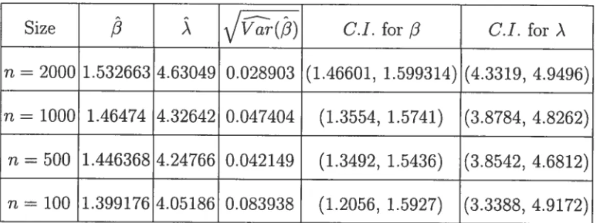
CONFIDENCE INTERVALS FOR THE PARAMETERS

We have used many sets of data and have found that when the pararneter becomes much smaller, the calculation speed is much siower. Thus to calculate tIre confidence intervals of the parameters \ and a, we generated several datasets

TABLE 5.2. Confidence interval for /3 and À witli 10 points

Size C.I. for

_/3

Ci. for À

n = 2000 1.532663 4.63019 0.028903 (1.46601, 1.599314) (4.3319, 4.9496) n = 1000 1.46474 4.32642 0.047404 (1.3554, 1.5741) (3.8784, 4.8262)

n = 500 1.446368 4.24766 0.042149 (1.3492, 1.5436) (3.8542, 4.6812)

n = 100 1.399176 4.05186 0.083938 (1.2056, 1.5927) (3.3388, 4.9172)

with À = 4.5 and c = 0.4. We use the resuits of Chapter 4 to caldulate the

confidence intervals of the two parameters c and À,

+t(l/2)(n - 2)()

& +t(l_/2)(fl — 2)().

Assume the significance level c is 5% and n = 10,

— 2) = t0975(8) 2.306,

we get the C.I. for the parameters o and À in Tables 5.2 and 5.3. Notice that the confidence intervals of the parameters become wider when n decreases.

5.3.

TEsTS CONCERNING

À

AND

o

We use the estimation resuits of the previous section to conduct a two-sided test concerning parameters c _{and À. The results are found in Tables 5.4 and 5.5} respectively.

1. To test

51

TABLE 5.3. Confidence interval for c with 10 points

Size C.I. for o

n = 2000 0.41506 0.00896627 (0.394384, 0.435736) n = 1000 0.383514 0.0180303 (0.341936, 0.425092)

n = 500 0.380229 0.014749 (0.346217, 0.4414241)

n = 100 0.39524 0.0299940 (0.326120, 0.464281)

TABLE 5.4. Test concerning c with 10 points

Size t” t0975(8) 2.306 conclusion ‘./Var(c) n 2000 0.41506 1.6796 2.306 accept H0 n = 1000 0.383514 -0.9144 2.306 accept H0 n = 500 0.380229 -1.3405 2.306 accept H0 n = 100 0.39524 -0.1587 2.306 accept H0

the test statistic is

vs Ha:d4O.4,

—

t

-

-The decision mie with this test statistic at the 5% significance level is: If t < _{t0975(8) 2.306, accept H0, i.e. OE 0.4,}

If > t0 (8) = 2.306, reject H0, i.e. 0.4.

2. To test

H0 : = 4.5

52 TABLE 5.5. Test concerning À with 10 points

Sïze to97(8) 2.306 conclusion

n = 2000 4.63049 0.133835 0.975 2.306 accept H0

n = 1000 4.32642 0.205090 -0.846 2.306 accept H0

n = 500 4.24766 0.179035 -1.409 2.306 accept H0

n = 100 4.05186 0.340105 -1.318 2.306 accept H0

the test statistic is

À—4.5 t*=

frar(À) Var(À)

note that we defined À = e3 and by the delta-theorem Var(À) ₌ e2VarCB).

The decision rue with this test statistic at the 5% significance Ïevel is: If t) < t0975(8) 2.306, accept H0, i.e. À = 4.5,

If t > t075 (8) 2.306, reject H0, i.e. À 4.5.

5.4. EFFEcT 0F TRUNCATION

In this section we will discuss the effect of data truncation. When the dataset is heavy tailed or with some extreme values, it must he truncated in order to obtain the estimators with the algorithm proposed.

We use the parameters c=0.4 and À=4.5 to generate samples of discrete stable random variables with different sample sizes (n=2000, n=1000, n=500 and n 100). These datasets are distributed with a heavy tau and the largest value of the observation in the sample are so large (when n = 2000, it is 446,630,588; when

n = 1000, it is 47,287,674; when n = 500, it is 1.24 x 108 and when n = 100,

it is 149,289) that we must cut the datasets somewhere in order to estimate the pararneters.

To conduct our calculation, we take:

{—0.9, —0.3,0.3, 0.9}

We put ail the calculation resuits in Tables 5.6 to 5.9 to compare the clifferences arnong the different situations.

Notice that at the same percentage of truncation, the absolute value of the relative errors of estimator ) increases when the sample size decreases.

With 8% or 10% truncation, when n = 2000, the absolute value of the relative

errors of estimator is 1.3%; when n 1000, it is 3.5%; when n 500, it is 7.7% and when n = 100, it is 12.1%.

With 20% truncation, when n = 2000, the absolute value of the relative errors

of estimator is 1.3%; when n = 1000, it is 8.1%; when n = 500, it is 10.0% and

when n _{100, it is 14.4%. We eau see that the absolute value of the relative}

errors of estirnator ) increases a lot with the decrease of the sample size n. In total, the sum of the absoute value of the relative errors of the two esti mators increase with the decrease of the sample size n.

With 15% truncation, when n 2000, the sum of the absolute value of the relative errors of the two estimators are 9.8%; when n 1000, it is 9.3%; when n = 500, it is 10.6% and when n = 100, it is 19.5%.

With 30% truncation, when n = 2000, the sum of the absolute value of the

relative errors of the two estimators are 23.1%; when n = 1000, it is 23.7%; when n 500, it is 23.7% and when n = 100, it is 33.9%.

Also notice that the relative errors of estimators increase when the percentage of truncation increases.

With n = 2000, the relative errors of estimator & increase from 3.8% (without

truncation) to 19.5% (with 30% truncation). At the same time, the absolute values of the relative errors of the parameter À, fluctuate from 2.9% to —3.7% with the percentage of truncation 8% to 30%.

With n = 100, the relative errors of estimator & increase from 3.5% to 16.9%

values of the relative errors of the estimator ? iucrease from 12.Ï9o to 16.9% when the percentage of truncation changed from 10% to 30%.

After using many different percentages of the truncation to estimate the pa rarneters, we conclude that with the percentage of truncation less than 15% and the sample size n > _{500, the estimation gives better resuits, the relative errors of}

TABLE 5.6. The effect of truncation on (n=r2000) estirna.tors relative errors without trunction cv0=0.41337 initial values À0 =4.6587 first iteration ci =0.41506 3.765 9’ À =4.63049 2.90

¾

with truncation c =0.426388 off 8

¾

À0 =4.57748 first iteration a=0.424454 À=4.55938

second iteration c= 0.424454 6.11

¾

À4.55938 1.320 ¶Y0 with truncation o=0.439585

off 15

¾

À0=4.50096 first iteration =0.438582 À=4.49284

second iteration c=0.438582 9.646

¾

À=4.49284 -0.159

¾

with truncation _o=0.450307 off 20 À0rr4.44248 first iteration c= 0.450093

À=4. 44256

second iteration o=0.450093 12.523

%

À=4.44256 -1.276

¾

with trunction a0 =0.476048 off 30

¾

À0 =4.31414 first iteration o= 0.477842 À=4.33432 second iteration =0.477842 19.461

¾

À=4.33432 -3.682

¾