HAL Id: hal-02137448
https://hal-mines-albi.archives-ouvertes.fr/hal-02137448
Submitted on 3 Jun 2019
HAL is a multi-disciplinary open access
archive for the deposit and dissemination of
sci-entific research documents, whether they are
pub-lished or not. The documents may come from
teaching and research institutions in France or
abroad, or from public or private research centers.
L’archive ouverte pluridisciplinaire HAL, est
destinée au dépôt et à la diffusion de documents
scientifiques de niveau recherche, publiés ou non,
émanant des établissements d’enseignement et de
recherche français ou étrangers, des laboratoires
publics ou privés.
Improving parcels transportation performance by
introducing a hitchhiker parcel model
Quentin Schoen, Franck Fontanili, Matthieu Lauras, Sébastien Truptil
To cite this version:
Quentin Schoen, Franck Fontanili, Matthieu Lauras, Sébastien Truptil. Improving parcels
trans-portation performance by introducing a hitchhiker parcel model. ICIEA 2019 - IEEE 6th
Interna-tional Conference on Industrial Engineering and Applications, Apr 2019, Tokyo, Japan. pp.420-429,
�10.1109/IEA.2019.8715142�. �hal-02137448�
Improving parcels transportation performance by introducing a hitchhiker parcel
model
Quentin Schoen*⸶, FranckFontanili*, Matthieu Lauras*, Sébastien Truptil*
*Centre Génie industriel, IMT Mines Albi81000 Albi, France
⸶Service logistique, Etablissement Français du Sang Toulouse, France
e-mail: {Quentin.schoen, franck.fontanili, matthieu.lauras, sebastien.truptil}@mines-albi.fr Abstract—Thanks to technological opportunities on data
acquisition, broadcast and treatment in real time, new logistics opportunities are emerging quickly. These opportunities are about to change deeply the way we transport parcels through hyper-connected and open networks. In order to monitor the logistics flows on these routes and hubs, new ways of thinking are developed, like the Physical Internet paradigm. Because the current transport management systems should not be able to deal with this complex and open environment, we have to design new ways of monitoring parcels on the network. We describe here the \emph{hitchhiker parcel model}, a new paradigm allowing each parcels to take advantage of the local opportunities and beware the risks. The targeted organization described and the underlying questions have to be evaluated through performance indicators. The first experiments presented here aims to give first insights about the model evaluation and its relevance.
Keywords- Physical Internet; Transportation; Monitoring; Simulation
I. INTRODUCTION
If we take a look to expected logistics trends [1] [2] [3] [4], it appears that the way we manufacture, store, distribute and use objects are about to change deeply. In fact, new technological opportunities like Internet of Things (IoT), cloud computing and data treatment abilities are enabling and fostering a relevant hyper-connection of any object to the World Wide Web.
This ability to equip any physical object with sensors (motion, temperature, pressure, location, etc.) and connect it easily and quickly to the Internet opens new opportunities in the logistics field. In particular for transport management, knowing the status and location of any actors and objects while they are spread in a region/country might be relevant to make appropriate decisions and meet new challenges. These technological opportunities are fostering an "anytime, anything, anywhere delivery" model [1] in order to satisfy the customers' needs. This model implies a network complexification and require from carriers agility. As a consequence, logistics activities breakdown between stakeholders and servicisation try to offer solutions to link the producer to the customer in effective, agile and efficient way, wherever they are and whenever the order is made. These trends are already visible in our everyday life with
resource sharing platforms (car and flat sharing, food delivery) and new delivery hubs as smart-lockers [5].
Despite these new trends, abilities and tools to manage the supply chain appear no longer adapted. In one of the first article presenting the Physical Internet paradigm, \cite{montreuil_toward_2011} illustrates some problems the \emph{current} logistics organisation is facing with on social, economical and environmental aspects. Air and packaging shipping, empty travel of vehicles and containers, carriers poor social working conditions, storage and transportation facilities misused and/or under-utilized are some of the symptoms presented in this paper. Meantime, despite the use of Transport Management Systems (TMS) by companies, we already observe lacks in the ability to deal with parcels in agile, effective and efficient manner [6]. These centralized and deterministic systems were not designed initially to deal with the upcoming network complexity and parcels traceability while numerous actors are successively in charge with different logistics means (vehicles, hubs, storage facilities, etc.). This leads, among other issues, to the symptoms described above, and it should be worse in few years if do not try to re-design these systems.
In order to answer the parcels transportation monitoring challenge, the Physical Internet paradigm [6] makes a list of disruptive recommendations and assumptions about the physical and informational standardisation of the supply chain. On the physical aspect it considers the encapsulation of the products in world-standard smart green modular
containers, handled, sorted, stored and transported through
adapted facilities. On an informational aspect it considers an hyper-connected world in which any object (container, vehicle, hub) may collect, treat, broadcast and receive data about its environment and/or state. In this situation, 3 types of monitoring are proposed:
1. A centralised monitoring: objects do not barely make decisions but relays informations to a agent 2. A pre-planned and de-centralised monitoring: the
containers follow one of the several itineraries planned before its departure
3. A fully de-centralised monitoring: objects make decisions about themselves autonomously
The first proposition looks like the current organisation with a higher visibility of the field situation in real time. The second one tries to take advantage of parcels and tags new abilities in order to decentralised the parcels routing decisions, following one of the pre-determined schedules. The third one allows a full autonomy of the parcels, depending on the real time surrounding environments.
These three monitoring types may be relevant, depending on the situation and the maturity level of the interacting objects. However, a centralized system may not be truly relevant to deal with specific parcels and amounts of local transportation opportunities and breakdowns between stakeholders. Secondly, considering the expected network complexity in terms of nodes and stakeholders diversity and quantity on one hand, and on another hand, the agility need in this almost unpredictable system, the second proposition with schedules to follow appears a bit tight. For these reasons, trying to take full advantage of IoT expected capabilities in term of data exchange and treatment in real time, we think relevant to consider in the following parts the third parcel monitoring system.
As a consequence, in this paper we address the following research question: “Does a parcel decentralised monitoring
system, based on smart and opportunistic parcels, increase the whole performance of the logistics network?”. To answer
that, we first describe the TMS evolution we think necessary to monitor the upcoming supply chain. Then, we describe the
hitchhiker parcel model, a new paradigm we think relevant
to deal with it. After that, we define a targeted organisation and some KPIs we should used to allow the parcel to find its way and make its decision itself. Next, we propose an experience plan and present the first experiments. Finally, we discuss this model and give perspectives to pursue these experiments.
II. BACKGROUND AND RESEARCH QUESTIONS
In this part, we describe in which extent the current TMS should evolve in order to pursue opportunities offered by the expected logistic environment. The first part gives on overview of the logistics opportunities and trends whereas the second one is focused on the current TMS approach and the required evolutions. In the third part we describe the
hitchhiker parcel model we propose and address the research
question.
A. New opportunities of the expected logistics network An hyper-connected network: For Small and Medium
Enterprise (SME) it may be expensive and it represents an important risk to buy a software to deal with their supply chain. For several years, the development of Software as a Service (SaaS) model is allowing a broader access to IT systems [7] [8], giving to SMEs the opportunity to choose precisely the functionalities they want [9] and take full advantage of cloud computing. In addition, the SaaS provider takes care of the infrastructure (hardware, network, updates) to support the software. Thus, a plug-and-play approach allows the SMEs to focus on their process and core system rather than on the software. Moreover, because of
this approach all the software units must be easily connected to other ones, which implies interoperability and foster data exchange. Little by little, this model creates an informational network through companies and customers, each one taking advantages of web services through Application Programming Interface (API).
Combined with the cloud computing and computing power increase, we assist for few years to the use of smart, small and affordable devices allowing people and objects to be connected anywhere at anytime [9]. The Internet of Things (IoT) development allows easier and more reliable data collection and broadcast from the field to a decision support system [10]. On a transportation point of view it means an ability to know the location and state of any parcel and vehicle any time. Considering that we are able to treat in real time these amount of data through Big Data technologies [11], the supply chain management should be deeply modified thanks to the real time understanding of the field situation.
This hyper-connection of the objects should allow the firm to reach the objective of “any-time, anywhere delivery
model” [1]. In fact, we are facing with a distribution
customization based on the consumers desires, which implies to build a network agile and reactive enough to fit with the consumer lifestyle. In order to reach this objective, the number of potential paths for a parcel between the firm and a consumer increase and the transshipments must not be a problem. The last mile delivery, the reverse logistic management, and the implementation of smart lockers [5] and shared warehouse are examples of facilities which should create a strong and agile network.
An open logistics network: In order to take advantage of
these opportunities, we assist for some years to a splitting of logistic activities, each stakeholders being responsible of its own perimeter. Thus, to deal with this complexity, companies are requiring services from 3-4-5PL providers [12] which aim to deal with their logistics activities (storage, transportation, product flow and supply chain management, optimization, etc.). Meantime, people are taking advantages of new services like shared car, shared flat, on demand transport, through new sharing economy platforms \cite{hamari_sharing_2016} which aim to link individuals needs with available abilities (Uber, Deliveroo, AirBnB, Blablacar, etc.). In both case, logistics activities are more and more considered as services offered by specialist companies and individuals as it is the case for SaaS.
This new way of thinking imply more collaboration and interfaces when a parcel needs to be transported from point A to point B. In fact, one actor may be responsible for the first transportation, a second one for the temporary storage on a transshipment hub, a third one for the last mile delivery and a forth one was responsible of real time data collection and traceability. Moreover all this transportation steps may be achieved by different transportation means like autonomous cars [14], platooning trucks systems [15], bicycle, drones, smart lockers [5] and shared [16] autonomous hubs. These opportunities imply an ability for
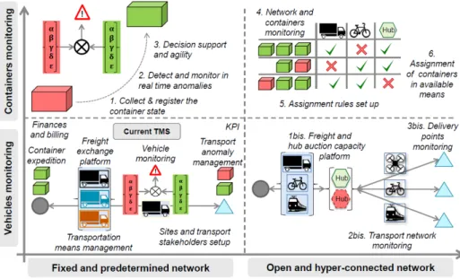
Figure 1. TMS evolution
parcels to be suitable for this automation and multi-modality which should contribute to improve the performance. Indeed, as explain by [9] the multimodality adds constraints on the package, the transport and storage conditions but allows to combine the advantages of each transportation mean used (flexibility of road haulage, high capacity of trains, lower costs of boats). In order to reach this physical intermodality, [6] wants to create and use standardise and smart
Pi-containers.
In this context of logistics activities servicization, splitting of responsibilities between several stakeholders, and use of different means more and more autonomous all the supply chain along, the logistics network appears more and more open and flexible. However, if we compare these expected needs and the TMS abilities, it seems that there is a gap to fill if we want tools able to deal with products all along the supply chain.
TMS origins: The Transport Management Systems were
initially created in 90s to provide "an enabling tool for the
safe and efficient operation of Freight Transport systems
[17]. According to [18] the major functionalities were: Following the vehicles location in real time and provide KPI about them
Providing a delivery proof
Monitoring the load through sensors and data collection (temperature, remaining capacity, etc.) In 2000s, the logistics network and activities became more complex, involving more and more actors responsible of specific perimeters. Because of this complexity, the interconnectivity between IT systems was not as efficient and relevant as it should have to be as [17] foresaw it. In order to solve these issues TMS functionalities and software components are becoming more interoperable for few years through plug-and-play components, available on SaaS platforms.
Current TMS functionnalities: As a consequence, the
current TMS are most of the time split in components "activated" or not, depending on the company needs: the carriers may need transportation means and drivers management module whereas the companies which need their goods to be transported by subcontractors may need freight and vehicle exchange platform and real time traceability. This structure offers more flexibility and allows even SME to access this kind of service.
The current most common functionalities are represented in Figure 1 [19]: form edition for each entity to be transported, vehicle rounds planning and optimizing, real time vehicle monitoring, vehicle and container track and trace of each transportation step, freight and vehicle exchange platform, transport quality management, transportation means management, finances and billing activities, etc.
Current TMS approach and limitation: One of the main
objective of the current TMS is to design in real time the most effective and efficient transportation rounds, minimizing the cost and maximizing the vehicle load. In addition, following the vehicle status and trailer/goods vehicle we consider that we follow the containers status. Nevertheless, it appears that this system does not prevent to ship a lot of air packaging [6] and multi-modality is still hardly considered because the current practices may slow down the delivery and endanger the parcel. The TMS organisation with rounds and vehicles monitoring does not foster agility [20] in case of unexpected event requiring products transported detour and real time decision. The whole logistics network is split between numerous competitive stakeholders networks with their own means which implies redundancy and inefficiency. Finally, this organisation and vehicle monitoring is often not sufficient
for sensitive products monitoring which require more precision about their environment (temperature, shocks, direction, etc.).
Considering the expected logistics environment described before, these current limitations should have a strong impact, preventing to monitor in a relevant way the parcel on the upcoming network.
B. Expected failures and key elements to improve
Taking into account the previous sections, we summarize here some key elements we should work on in Figure 1 [19]:
Parcels monitoring: Following in real time each parcel status and location. Ability to make decision about them considering all their constraints and their environment.
Vehicles and hubs monitoring: Taking advantage of any storage and load displacement capability in order to improve the whole network effectiveness and efficiency.
Automatic parcel assignment in the available means: Defining rules based on KPIs and compatibility between parcels and vehicles/hubs in order to assign automatically the first ones to the second ones.
Considering the expected capabilities of data collection and treatment technologies, on one hand, and on the other hand, the major logistics trends described above, these TMS evolution appear feasible and relevant.
C. The hitchhiker parcel model
Description: In this hyper-connected and open
environment, it appears to us (cf. Introduction) that a decentralised and opportunistic model to monitor parcels would be relevant. In this situation, each parcel may be compared with a hitchhiker. In fact, it takes advantages of the opportunities and beware the risks, without knowing in advance its itinerary to reach the recipient, as a hitchhiker during its trip. Analysing its environment and knowing its products constraints, each parcel should be able to make relevant decisions about vehicles to take and hubs to be stored in, waiting for another displacement opportunity. As it is anticipated in the future by [6], we consider distributed multi-segment intermodal transport as the major transport organisation. This means that on the whole network vehicles are mostly similar to shuttles between hubs able to deal with different vehicle types.
In our study, considering the collaborative economy and platforms which already emerged, we think relevant to take also into account the vehicles that did not initially planned to carry parcels. The vehicles flow, regardless of their type, is considered as load capacity displacement. Any vehicle, in particular private ones, passing nearby the hub a parcel is stored in, planning to pass close to another one considered interesting by the parcel to get closer to its destination, is susceptible to carry it. To summarize, we consider the parcels displacement needs on one hand, on the other hand, we consider the displacement and storage means susceptible to meet the parcels needs.
Decision making: Currently each carrier takes in charge
the parcel he has been ordered for. In the hitchhiker parcel
model the parcel decides itself whether or not a
transportation availability is relevant for it. Thus, in this context we have to answer the following questions:
1. How does a parcel decide that a transportation opportunity is relevant for it?
2. When a vehicle offers a transportation opportunity to parcels, how does the vehicle decide the ones it takes in charge if the interested parcels number / volume / weight exceeds the vehicle capacity? Our goal is to define a new way of monitoring the parcels in the upcoming logistics environment, because we expect the current monitoring systems inappropriate to deal with it. To answer this challenge, we make the assumption that the Physical Internet opportunities and the hitchhiker parcel
model are adapted. As a consequence, in order to evaluate
the relevance of our model, we have to answer the following research question: “Does a parcel decentralized monitoring
system, based on smart and opportunistic parcels, increase the whole performance of the logistics network?
To answer it, we have to describe the targeted organization and KPIs that parcels, vehicles and hubs may use to make decisions. In fact, depending on KPIs and decision making algorithms used, the parcels behavior will change, so will the global logistics network performance. Experiments in section IV are designed to answer the research question, evaluating the performance of this model.
III. PROPOSAL
A. The hitchhiker parcel and sensitivity
In the described hitchhiker parcel model, each parcel must be able to track physical data about its environment, exchange them with the surrounding elements (vehicles, hubs), interpret them and make decisions based on these treatments by itself.
As a hitchhiker, each parcel may be different and more or less affected by its environment and unwanted events like delay or unsuitable transportation conditions. The
Merriam-Webster dictionary define sensitivity as:
the quality or state of being sensitive: such as the capacity of being easily hurt
Thus, in order to distinct the parcels we define a
sensitivity factor si which aims to make a difference between
a parcel we should monitor strictly and another one which may not be affected as much by an unexpected and/or unwanted event. This factor is set arbitrarily between 1 (ie. low sensitivity) and 10 (ie. high sensitivity) and depends on the parcel internal factors (product fragility, scarcity, dangerous nature, cost, thermal/mechanical/chemical/... insulating capacity of the container, etc.) and external ones (impacts of a delivery issue on the parcel recipient). In the further KPIs description we use this factor dimensionless to discriminate the parcels and set a priority between them.
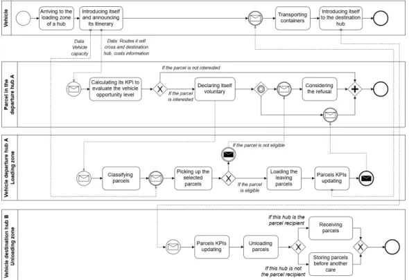
Figure 2. Parcel transportation: Expected scenario
B. Targeted organisational model
Common shipping process without transshipment: This
process gathers in a chronological way the different tasks required in order to send products inside a parcel from site A (vehicle departure hub) to site B (vehicle destination hub) directly with one transportation step:
The sender (shipment tasks):
- T1: Prepares the parcel storing the products inside and editing the documentation associated.
- T2: Stores the "ready to go" parcel in an adapted storage area.
The carrier (transportation tasks): - T1: Arrives on site A
- T2: Takes in charge the parcel - T3: Transports the parcel
- T4: Delivers it in an adapted storage area on its destination site
- T5: May take in charge other(s) parcel(s) to deliver them on another site
- T6: Leaves the site The receiver (receipt tasks):
- T1: Opens the package and take the products In case of transshipment, a second carrier repeats the same process with parcels left on this site by the first one. In any case, we do not consider in the whole paper the steps achieved by the sender nor the recipient because it does not belongs to the transportation steps.
In our proposal, the key questions (cf. II-C) are asked in carrier's task T2 when several options are possible for the parcel.
Organizational model: We describe in the figure 2 the
organizational model with BPMN language. We make the assumption that vehicles arrive empty in the loading area of the departure site and unload all the parcels they have transported in the destination hub. As we see it on the diagram, we can split the decision process in 3 steps:
1. Arrived vehicle broadcast of its identity and route to the parcels on the site
2. Parcels KPI calculation and decision on the willingness to take advantage of this transportation opportunity
3. Classification of the voluntary parcels in case of vehicle capacity issue
We observe the data exchange between the vehicle and parcels once a new opportunity appears. The decision of being volunteer for this transportation opportunity is calculated considering the vehicle parameters, the itinerary parameters (edge and destination hub) and the parcel parameters (state, destination, sensitivity factor, etc.).
C. KPIs to make a decision
We describe in the following parts some KPIs which appear to us relevant for a parcel to decide whether or not a vehicle represents an opportunity and to classify the volunteer parcels. We make the assumption that any parcel must reduce as much as possible the time spent between the sender and the recipient. In fact, during transportation and transshipment steps parcels are expected by their recipients and exposed to risks that may injured products inside, in particular if the sensitivity factor si is high.
In the following parts, for each parcel, we settle the first step (n=1) when a vehicle leaves the sender's hub, and the last one (n=2N+2) when a vehicle stops in the parcel's recipient hub, considering N as the number of transshipment hubs.
Real time and step sensitivity: In order to take into
account the sensitivity of each parcel in the shipments monitoring, we define in (1) the real time sensitivity for each parcel i, just after the step n, which means between
.
(1) Based on (1) we define in (2), the step sensitivity of parcel i between steps n and n+1.
(2) Based on historical values registered by former parcels on the same place, if a parcel is able to estimate the time it will spend between two steps (loading - unloading or unloading - loading) it is able to estimate in advance its potential future step sensitivity.
Cumulative real time and step sensitivity: Based on the
former equations we can add up the step sensitivities all the transportation steps along in order to compare the parcels, whatever their previous itinerary were. This is possible if parcels considered crossed at least one transshipment site, ie. N>1. Thus, we define the cumulative real time sensitivity of each parcel i between its departure from the sender site and any given moment in (3):
(3) Based on (3) we define in (4), the cumulative step
sensitivity of parcel i considered at step n.
(4) As a consequence, (3) may be simplified with (5):
Equation (5) registers the transportation duration of each parcel so far and take into account their sensitivity to compare them. The highest this value is, the fastest the parcel
should be transported to its recipient. However, we do not know if the situation is urgent or not, the parcel may have plenty of time to reached the recipient.
Maximum transit time: In order to fill this gap, we define
for each parcel i. This is the difference between the latest arrival time (LA) and the earliest departure time (ED. Thanks to we define as the portion of available time
consumed in real time} in (6) which add the time consumed
between the earliest departure and the first care, and the time consumed in transportation step(s) so far.
(6) If their is no transshipment, (6) is simplified with (7).
(7)
Finally, we can calculate the portion of available time
consumed on step n} with (8).
(8) Thus, this indicator is useful to detect the parcels which should be transported quickly in order to respect their latest arrival time. However, this indicator does not take into account the network ability to forward the parcel on time. In fact, even if = 0.8, if this parcel is very close to its recipient it might be more relevant to make it wait, compared with another one with = 0.5 but very far from the recipient.
NB: The sensitivity factor is not part of these equations not
to make them more complex but it could be a perspective.
Network conveyance capacity: Considering the hitchhiker parcel model we do not know in advance edges
and hubs a parcel will pass through to reach its destination. Nevertheless, we can use the shared historical data about previous parcels which pass through these links. In fact, thanks to these data we may predict how much time will be necessary to leave a hub and reach another one, regardless the itinerary. We define as the average time for a
y type parcel to travel from step n to step m in a vehicle type z. is defined between two steps which implies that it is a discrete variable. To define , the network
conveyance capacity, we use to evaluate the time already consumed and the time that should be consumed to reach the recipient site in (9). In this specific case, the step m is the recipient.
Figure 3. Experimental network required time
(9) This indicator is useful if compared to 1:
If Λ << 1, apparently the parcel will arrive on time to its destination
If Λ ≈ 1, apparently the parcel should arrive on time to its destination but the probability is lower than the first one
If Λ >> 1$, apparently the parcel will be late to reach its destination, an alternative solution should be found to avoid this.
This indicator appears as a good one to evaluate in real time a parcel status. Combined with and it allows the parcel and the vehicle to evaluate the urgency of parcel to be taken in charge.
In the organisation we described so far, parcels may go through several hubs to reach their destination. In order to determine if a hub is relevant for a parcel to get closer to the recipient hub we define 4 steps:
n is the potential loading step of a parcel $i$ in its
current hub
v is the step of delivery on the temporary hub v+1 is the loading step on the temporary hub m is the delivery step of a parcel i on its recipient
hub
With these steps we define , the convergence
rate of type y parcel which is offered to go on site v to reach
its destination m in (10).
(10) Equation (10) compares two options:
1. The estimated time to leave from the current site to the vehicle destination added to the time spent there and the time to go from there to the parcel destination
2. The average time to leave from the current site and go the destination site
It is important to understand that all the are considered regardless to the itinerary. allows us to evaluate if a vehicle destination is relevant for a parcel. Once again, this indicator is useful if compared to 1:
If Cv << 1, it is really interesting to take this transportation because it shortens the time to reach the destination compared with a direct path
If Cv = 1, the vehicle destination may be the parcel destination. If it is not, the detour is not disadvantageous from a time perspective (it might be less interesting on a cost or risk exposure perspective).
If Cv >> 1, the vehicle destination represents a detour time consuming, compared with an average lift from the current site to the parcel destination site.
Based on this, we can imagine a Cv maximum level, above which a parcel does not even consider the transportation opportunity because the vehicle destination would represent a too-long detour.
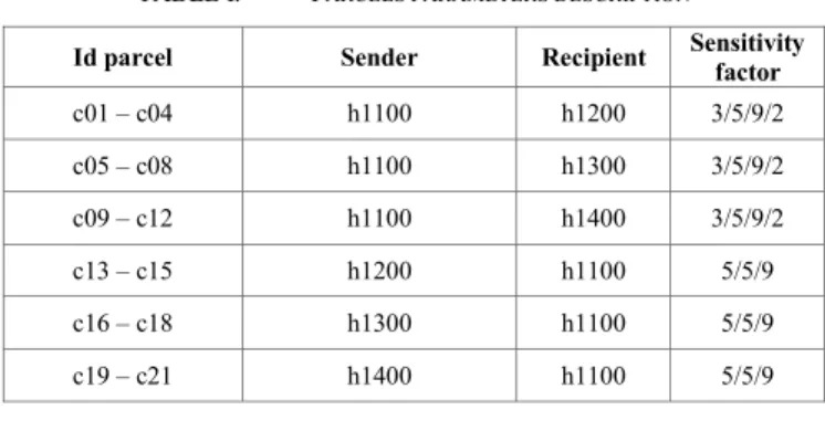
TABLE I. PARCELS PARAMETERS DESCRIPTION
Id parcel Sender Recipient Sensitivity factor
c01 – c04 h1100 h1200 3/5/9/2 c05 – c08 h1100 h1300 3/5/9/2 c09 – c12 h1100 h1400 3/5/9/2 c13 – c15 h1200 h1100 5/5/9 c16 – c18 h1300 h1100 5/5/9 c19 – c21 h1400 h1100 5/5/9
IV. EXPERIMENT AND DISCUSSION
In order to answer our research question, we define an experimental plan to measure in what extent the hitchhiker
parcel model improves the performance of the whole
expected network. The main idea is to compare current optimal rounds organisation with our model, modifying and improving the KPIs used and the decision making algorithms. We present here the first experiment we led to measure in a simple use case if our model may be relevant. A second experiment is led in order to improve the effectiveness and discuss the targeted organisation. We built from scratch a discrete-event simulation model runned by Witness© in order to lead these experiments. This simulation platform is relevant because the number of parameters (about vehicles, parcels, hubs, routes) we can play with is high. In addition, we need to understand precisely, step by step, what would happen with each decision making algorithms.
A. Description of the experiment and assumptions
Being the first experiment we run on this model we first make it simple to be able to analyse the results and consistent with a real use case. In fact, the situation described is based the blood supply chain [21] where a major hub (the production plant) needs to send different products to distribution centres. These distribution centres are meantime
TABLE II. FIRST EXPERIMENTAL RESULTS Id Ωhh Ωr Ωr - Ωhh Ψh Ψr Ψr - Ψr c01 18 18 0 0.52 0.26 -0.26 c02 30 30 0 0.52 0.26 -0.26 c03 54 54 0 0.52 0.26 -0.26 c04 12 12 0 0.52 0.26 -0.26 c05 156 48 -108 1.62 0.5 -1.12 c06 260 80 -108 1.62 0.5 -1.12 c07 468 144 -324 1.62 0.5 -1.12 c08 104 32 -72 1.62 0.5 -1.12 c09 36 84 48 0.62 0.79 0.17 c10 60 140 80 0.62 0.79 0.17 c11 108 252 144 0.62 0.79 0.17 c12 24 56 32 0.62 0.79 0.17 c13 30 170 140 0.33 1.12 0.79 c14 30 170 140 0.33 1.12 0.79 c15 54 306 252 0.33 1.12 0.79 c16 100 120 20 0.71 1.12 0.4 c17 100 120 20 0.71 1.12 0.4 c18 180 216 36 0.71 1.12 0.4 c19 60 60 0 0.95 1.12 0.17 c20 60 60 0 0.95 1.12 0.17 c21 108 108 0 0.95 1.12 0.17
collection centres of raw materials. This organization is based on the well-known milk-run problem [22].
The network is made of 4 sites, 1 major and 3 secondary ones. The transport commonly used in this situation is a pick-up and delivery rounds, leaving first from the major site and visiting all the secondary sites one after the other. If a parcel needs to be transported from a secondary site to another one, it might needs to be stored temporarily on the major site before the second same round begins.
The figure 3 represents this network. First, we define the required time to cross each edge (yellow continuous lines). Secondly we define the average time spends by a parcel on a hub in the hitchhiker parcel model (grey circles on hubs). Considering a vehicle stays 2 time units on a hub (yellow circles on hubs) and might be anywhere when a parcel is ready to go, we use the average between the half of a return trip to its both surrounding site. For instance, the calculation for 8 on h1200 is: ((6+2+6)/2)+((8+2+8)/2)/2. The yellow
dotted lines define the time to go from one hub to the other one but does not represent a passable edge. The average time on them is the average between both paths in the hitchhiker
parcel model. For instance, the calculation for 28 between
TABLE III. SECOND EXPERIMENTAL RESULTS
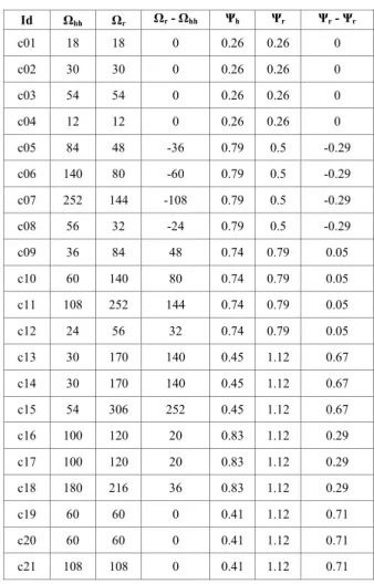
Id Ωhh Ωr Ωr - Ωhh Ψh Ψr Ψr - Ψr c01 18 18 0 0.26 0.26 0 c02 30 30 0 0.26 0.26 0 c03 54 54 0 0.26 0.26 0 c04 12 12 0 0.26 0.26 0 c05 84 48 -36 0.79 0.5 -0.29 c06 140 80 -60 0.79 0.5 -0.29 c07 252 144 -108 0.79 0.5 -0.29 c08 56 32 -24 0.79 0.5 -0.29 c09 36 84 48 0.74 0.79 0.05 c10 60 140 80 0.74 0.79 0.05 c11 108 252 144 0.74 0.79 0.05 c12 24 56 32 0.74 0.79 0.05 c13 30 170 140 0.45 1.12 0.67 c14 30 170 140 0.45 1.12 0.67 c15 54 306 252 0.45 1.12 0.67 c16 100 120 20 0.83 1.12 0.29 c17 100 120 20 0.83 1.12 0.29 c18 180 216 36 0.83 1.12 0.29 c19 60 60 0 0.41 1.12 0.71 c20 60 60 0 0.41 1.12 0.71 c21 108 108 0 0.41 1.12 0.71
h1100 and h1300 is: ((6+8+8)+(12+12+10))/2. Each edge may
be used both directions.
We consider just one type of vehicle, the same for both cases (rounds and hitchhiker parcel model), with the same speed and an infinite capacity.
We consider that all parcels are the same in term of weight, dimensions and maximum transportation duration (earliest departure ED = 0). The only differences are the sender, the recipient and the sensibility factor, depending on the parcel type. We consider that the major hub h1100 sends 4
parcels to each hub. Meantime, each site sends 3 parcels. We summarize these parcels sending in table I.
B. Round description
In order to compare the effectiveness of both models, rounds and hitchhiker parcel model, we begin to design a simple pick up and delivery (P&D) round. We consider that all the parcels are available on each site at the beginning (t=0) and the vehicle arrives at t=3, because the round is well designed to suit the needs. As define hereafter the vehicle arrives on hub h1100 (t=3), it loads all the parcels, leaves the
hub (t=5), arrives on hub h1200 (t=11), unload the parcels
whose the recipient is this site and loads the parcels addressed to hub h1100. Then, it leaves the hub (t=13), etc.
C. The hitchhiker parcel model, first experiment
Experiment: With parcels described in Table I we test
here the model defined above, considering as a decision on the willingness to take advantage of a transportation opportunity: Cv ≤ 1. In this case the parcel is eligible to the transport, in the other case it stays on hub waiting for another opportunity. We checked before that this rule does not prevent a parcel to reach its destination thanks to at least one specific way. We used 4 vehicles equivalent to shuttles, each one responsible of an edge. When the experiment begins, each of them leaves a hub empty, travelling to the next one.
We gather on Table II the results and a comparison with the round. KPIs used to compare the scenarios are the
cumulative step sensitivity Ω and the portion of available time consumed Ψ. The first one indicates for each parcel how
long was the trip and the second one indicates when it took place.
Analysis: As we can see, Ψhh > Ψr for parcels c01 to c04
because even if these 4 parcels took the same time to travel from h1100 to h1200 (Ωhh = Ωr) with both organisations, the
round took them first. Secondly, Ωhh is very high for parcels
c05 to c08. This implies they waited a long time on hub h1200
to go from h1100 to h1300, after travelling with c01 to c04.
On the contrary, all the other parcels took less time with the hitchhiker parcel model than with the round Ωhh < Ωr).
Parcels c09 to c12 either stayed all the round along transported
in the vehicle waiting for h1400, either took the vehicle which
go back and forth from h1100 to h1400. The second option takes
less time than the first one. Conclusions are the same for c13
to c15, the travel is shorter taking directly the vehicle between
h1100 to h1200 than waiting into the vehicle to reach h1100.
Parcels c16 to c18 are an example of the parcel selection
rule based on Cv. In fact, the travel is shorter passing by h1200
than h1400. Thus, thanks to a vehicle available at the right hub
at the right moment these parcels took less time to go from h1300 to h1100 with the hitchhiker parcel model and arrived
before the round (Ψhh < Ψr).
Finally, parcels c19 to c21 arrived before the round with
the hitchhiker parcel model but consumed a very long time (0.95). This is explainable by the fact that the vehicle initial conditions (leaving h1400 empty) are not optimal for these
parcels. As for the round this is logical, they waited for the vehicle to arrive from h1300.
Conclusions: As we can see, the initial conditions have a
major impact on the results. In fact, in the hitchhiker parcel
model experiment, the vehicle synchronisation is essential
not to make parcels waiting too much time on a hub. In a larger extent, the highest is the frequency of vehicle visits on a site, the best effective this organisation will be. Moreover, as the parcels c16 to c18 demonstrate it, passing by a hub with
a transshipment may be more efficient than waiting in a hub a round to come. In fact, as for the parcels leaving from h1200
and h1400, the frequent vehicle visits in both direction creates
several opportunities to reach hub h1100. Finally, to make this
system efficient, it appears necessary to share the vehicles with other company needs and to consider private vehicles to fill them as much as possible . In fact, whereas the round
travelled 36 time units, the hitch-hiking vehicles consumed 214 time units.
D. The hitchhiker parcel model, second experiment Experiment: In this second experiment, considering that
frequency and initial conditions are key elements for the
hitchhiker parcel model to be effective, we change them. The
major improvement are the initial conditions, considering that the 4 vehicles are similar to the round, arriving on a site after 3 time units and offering a load capacity displacement to another hub. We do not change anything else in the
hitchhiker parcel model experiment. Nothing is changed in
the round experiment.
Analysis: Parcels c01 to c04 obtain logically the same
results with both organisation. A vehicle arrives (t=3), leaves h1100 to reach h1200 and unload parcels. Parcels c05 to c08 need
more time with the hitchhiker parcel model compared with the round (Ωhh > Ωr), waiting on h1200 but the synchronisation
is far better than before. In fact, in total these 4 parcels use 532 time units versus 988 in the first experiment. In addition, Ψhh as decreased from 1.62 to 0.79 which confirms that they
are cared fastest than in the first experiment. Parcels c09 to c12
require logically the same time than in the first experiment, as it is the case for parcels c13 to c15 and c19 to c21. Indeed
they just need to be transported one time directly to h1100,
thus Ωhh does not change, compared with the first
experiment. Finally, we notice that Ψhh raises a bit, compared
with the first experiment for parcels c09 to c18. This is
explained by the initial conditions change, vehicles arriving 5 time units later.
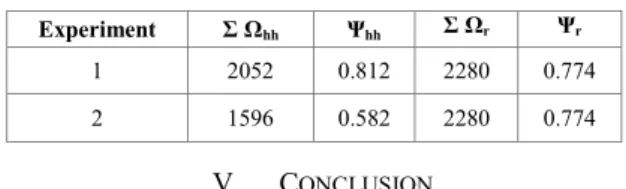
Conclusion: This second experiment allow us to
conclude that in this very simple case initial conditions and vehicle hub visits frequency are key elements. The results are presented in Table IV. These encouraging results confirm that the model we present in this paper may be relevant in the expected logistics environment. The vehicle synchronisation is essential and have a direct impact on the network capacity to dispatch parcels. Indeed, contrary to the first experiment, vehicles in the hitchhiker parcel model uses 92 time units instead of 214. Hubs with the highest vehicle opportunities will be apparently preferred to less visited ones. Another option could be to signal to any vehicle around a hub that a parcel just arrived on it and broadcast its parameters. This would allow parcels not just to wait for a vehicle but inform and encourage the transportation means to pay attention to this need.
TABLE IV. EXPERIMENTS COMPARISONS
Experiment Σ Ωhh Ψhh Σ Ωr Ψr
1 2052 0.812 2280 0.774 2 1596 0.582 2280 0.774
V. CONCLUSION
As we demonstrate it, the upcoming logistics environment is about to offer new opportunities the current management systems should not be able to seize. In order to
meet the upcoming logistics challenges offered by new technologies, required by the ineffectiveness of the current system and customers wishes, new way of thinking like the Physical Internet emerged. Based on these assumption, our model aims to provide a original way of monitoring parcels on an open and hyper-connected network. The hitchhiker
parcel model we built and evaluated is the first step before
other experiments. The first ones we present here prove that on a simple case, this model may be relevant to carry parcels on time. In addition, as we presented it, this decentralised system based on smart and opportunistic parcels could increase the whole performance of the network. In this simple case, compared with the round organisation, parcels were transported less time and delivered in average sooner. However, the efficiency must be improved, considering crowd-sourcing transportation and mixing all the parcels to raise the vehicles fill rate. In fact, the first experiments lead to an important increase of the time units consumed by vehicles.
This model have to be improved and its effectiveness confirmed by broader and more complex experiments. This future research works will compare the current situation with the expected one considering for example:
Vehicles capacity issues
A bigger network with more hubs, edges and vehicles
Cost relevant indicators to monitor the parcel which owns a pot
Risks relevant indicators to monitor the parcel through secure hubs and edges
New parcel choices algorithms combining time, cost and risks indicators
Unwanted event during transportation steps and parcel surveillance to measure agility capabilities Ephemeral hubs settled dynamically by vehicles exchanging parcels without long term storage facilities
Etc.
Future paper addressing these parameters and limitations should allow a better understanding of this kind of model capabilities and relevant implementation perimeters.
VI. REFERENCES
[1] “Logistics trend radar 2016.” [Online]. Available: http://www.dhl.com/content/dam/downloads/g0/aboutus/logistics insights/dhl logistics trend radar 2016.pdf
[2] “Logistics trend radar 2018.” [Online]. Available: https://www.logistics.dhl/content/dam/dhl/global/core/documents/pdf/ glo-core-trend-radar-widescreen.pdf
[3] M. Savelsbergh and T. Van Woensel, “50th anniversary invited article—city logistics: Challenges and opportunities,”vol. 50, no. 2, pp. 579–590. [Online]. Available: http://pubsonline.informs.org/doi/10.1287/trsc.2016.0675
[4] D. T. Matt, E. Rauch, and P. Dallasega, “Trends towards distributed manufacturing systems and modern forms for their design,” vol. 33, pp. 185–190. [Online]. Available: https://linkinghub.elsevier.com/retrieve/pii/S2212827115006770
[5] L. Faugere and B. Montreuil, “Hyperconnected pickup & delivery locker networks,” in Proceedings of the 4th International Physical Internet Conference.
[6] B. Montreuil, “Toward a physical internet: meeting the global logistics sustainability grand challenge,” vol. 3, no. 2, pp.71–87. [Online]. Available: http://link.springer.com/article/10.1007/s12159-011-0045-x
[7] T. Weber, “Cloud computing goes mainstream.” [Online]. Available: https://www.bbc.com/news/10097450
[8] D. O’sullivan, “Software as a service: developments in supply chain IT,” vol. 9, no. 3, pp. 30–3.
[9] I. Harris, Y. Wang, and H. Wang, “ICT in multimodal transport and technological trends: Unleashing potential for the future,” vol. 159, pp. 88–103.
[10] M. E. Porter and J. E. Heppelmann, “How smart, connected products are transforming competition,” p. 23.
[11] S. F. Wamba, S. Akter, A. Edwards, G. Chopin, and D. Gnanzou, “How ‘big data’ can make big impact: Findings from a systematic review and a longitudinal case study,” vol. 165, pp. 234–246.
[Online]. Available:
https://linkinghub.elsevier.com/retrieve/pii/S0925527314004253 [12] A. V. Vasiliauskas and G. Jakubauskas, “Principle and benefits of
third party logistics approach when managing logistics supply chain,” no. 2, p. 6.
[13] J. Hamari, M. Sj¨oklint, and A. Ukkonen, “The sharing economy: Why people participate in collaborative consumption”vol. 67, no. 9, pp. 2047–2059. [Online]. Available: https://onlinelibrary.wiley.com/doi/abs/10.1002/asi.23552
[14] B. Van Meldert and L. De Boeck, “Introducing autonomous vehicles in logistics: a review from a broad perspective.” [Online]. Available:
https://lirias.kuleuven.be/bitstream/123456789/543558/1/KBI 1618.pdf
[15] E. Chan, P. Gilhead, P. Jelinek, P. Krejci, and T. Robinson, “Cooperative control of SARTRE automated platoon vehicles.” [Online]. Available: https://trid.trb.org/view/1263454
[16] R. Franklin and S. Spinler, “Shared warehouses – sharing risks and increasing eco-efficiency,” vol. 10, no. 1, pp.22–31. [Online]. Available: http://link.springer.com/10.1007/s12146-011-0070-3 [17] G. Giannopoulos, “The application of information and
communication technologies in transport,” vol. 152, no. 2, pp. 302– 320. [Online]. Available: http://linkinghub.elsevier.com/retrieve/pii/S0377221703000262 [18] V. Zeimpekis and G. M. Giaglis, “Urban dynamic real-time
distribution services: Insights from SMEs,” vol. 19, no. 4, pp.367– 388.
[19] Q. Schoen, S. Truptil, M. Lauras, and F. Fontanili, “A new approach for supply chain management monitoring systems adapted to crisis,” in Working Conference on Virtual Enterprises.Springer, pp. 512–523. [20] A.-M. Barthe-Delanoe, M. Lauras, S. Truptil, F. B´enaben, and H. Pingaud, “A platform for event-driven agility of processes: A delivery context use-case,” in Collaborative Systems for Reindustrialization, ser. IFIP Advances in Information and Communication Technology, L. M. Camarinha-Matos and R. J. Scherer, Eds. Springer Berlin Heidelberg, pp. 681–690.
[21] Q. Schoen, F. Fontanili, A.-G. Anquetil, S. Truptil, and M. Lauras, “Tracking in real time the blood products transportations to make good decisions,” in ISCRAM 2017 - 14th International Conference on
Information Systems for Crisis Response and Management, pp. 173– 180.
[22] G. S. Brar and G. Saini, “Milk run logistics: Literature review and directions,” in WCE 2011, vol. I, p. 5.