OATAO is an open access repository that collects the work of Toulouse
researchers and makes it freely available over the web where possible
This is a publisher’s version published in: http://oatao.univ-toulouse.fr/24147
To cite this version:
Tchangani, Ayeley A Model to Support Risk Management
Decision-Making. (2011) Studies in Informatics and Control,
20 (3). 209-220. ISSN 1220-1766
Official URL:
https://doi.org/10.24846/v20i3y201102
1. Introduction and Statement
1.1. Introduction
Facing an adverse event (an earthquake, a hurricane, a malicious action, the failure of a machine, etc.), managers of an entity (a physical system, a human organization, etc.) will be concerned with the impact on their objectives or stakes that we will generically refer to as their desires in this paper. These desires are the main issues that will guide actions which managers may consider in order to reduce as much as possible the negative impact of the event. But the outcomes of these actions are always subject to uncertainty creating then a risky situation. So risk can be defined as the uncertainty of the consequences or outcomes of events and/or actions. To correctly address uncertainties mainly in terms of mathematical tools to represent them, we need to know their nature.
Roughly, there are three types of uncertainties briefly explained below.
Epistemic uncertainty: this type of uncertainty is
due to incomplete knowledge and it ranges from deterministic knowledge to complete total ignorance; for instance the question "are genetically modified organisms dangerous for human being?" is subjected to epistemic uncertainty. Epistemic uncertainty can be reduced or transformed to variability uncertainty provided that the analyst or decision maker
disposes of time and/or resources to do studies or to observe the system; decision making problems where this type of uncertainty also known as severe uncertainty occurs are generally solved by worst case analysis or Wald's maxi/min principle [23]; we are not going to address this kind of uncertainty in this paper.
Variability uncertainty is due to the inherent variability in the behaviour of some components of a decision making problem (environment, humans, outcomes, etc.). The uncertainty related to a question such as "what will be the magnitude of the next earthquake in Japan?" can be considered to be subjected to variability uncertainty. Contrary to epistemic uncertainty, variability uncertainty is not reducible and must be adequately addressed by mathematical tool in any rational decision making problem. The appropriate mathematical tool to manage variability uncertainty is the theory of probability and its connected graphical tools such as Bayesian networks and influence diagrams [9, 14].
Fuzzy uncertainty: this uncertainty comes
mainly from the impossibility of humans to precisely define events or variables and/or the fuzzy discretization of continuous variables. Indeed, humans usually express their opinions in terms of linguistic variables such as: this is a tall person, this season we expect our sale to be high, etc. The mathematical tool to address
A Model to Support Risk Management Decision-Making
Ayeley P. Tchangani1,2 1
Université de Toulouse, Université Toulouse III - IUT de Tarbes, 1 rue Lautréamont, 65016 Tarbes Cedex, France.
2
Université de Toulouse, Laboratoire Génie de Production - ENIT, 47 Avenue d’Azereix, 65016 Tarbes Cedex, France.
Abstract: This paper considers the issue of designing a framework to efficiently manage the risk due to some adverse
events an organization or a system may face. Risk comes from human being’s incapacity to predict the consequences or outcomes of some external events and/or their own actions, or to express precisely their knowledge about things. Thus, risk is linked to uncertainties that are inherent to almost all activities of human being. Designing an effective risk management decision making framework necessitate to correctly address these uncertainties in terms of appropriate mathematical tools along with procedures to identify variables (risk factors, state of the system, consequences, objectives or stakes, possible actions, etc.) impacting decision process and relationships linking them and finally aggregating approaches to present high level managers with concise information. In this paper we will use a meta-matrix analysis to identify relationships between previously determined variables, Bayesian networks and influence diagrams, graphical tools that permit easy representation of probabilistic relationships (independence, causality, correlation, etc.) between variables to quantify these relationships, and Choquet integral as an aggregation tool.
fuzzy uncertainty is naturally the fuzzy set theory (see [21]).
In this paper we will be concerned by variability and fuzzy uncertainties.
Integration of risk factors in decision making or risk informed decision making is receiving a great attention by researchers and decision makers in many domains such as engineering (designing technical systems that mitt some requirements in terms of safety), finance (set up norms to monitor finance activities in order to avoid companies collapse), environment (develop sustainable agriculture and natural resources extraction actions), science and medical research (monitoring scientists activity by the society to avoid creating new threats) because national and international opinions are being more and more sensible to risk issues from all human activities. The purpose of this paper is to develop a risk management framework and a generic model that can be used to support making and planning pre-active, reactive or proactive decisions.
Pre-active decisions: these decisions consist in
doing things to prepare the entity under consideration to face potential adverse events (one knows that such events will occur soon or later). Actions such as transferring risk by contracting insurances, editing anti-seismic construction norms in the case of natural disasters or prudential norms such as those of Bâle II (see for instance [22]) concerning banking activities, preparing population on how to behave in the case of an earthquake, constructing and organizing emergency facilities, etc. are pre-active decisions.
Reactive decisions: reactive decisions consist in
real time actions when the adversary events are present; decide which emergency unit will be affected to which zone or region during an earthquake; which credit to reduce by a government when an unplanned event such as petrol price raise occurs, renegotiating contracts with partners when they fail to realize their duties or redirecting activities in a supply chain for instance, etc. constitute reactive decisions.
Pro-active decisions: they consist in things that
must be undertaken to force a particular situation (avoiding catastrophic situation for instance). Risk prevention using redundancy for instance (to avoid the failure of a function or component in an industrial system), destroying or weakening terrorist groups such
as Al Quaida by military actions in order to prevent events like that of 9/11 participate to such proactive decisions.
Risk and uncertainty are fundamental elements of modern life so they must be managed effectively to protect people from injury and to permit the development of reliable, high-quality products. Today an ever-increasing number of professionals and managers in industry, government, and academia are devoting a larger portion of their time and resources to the task of improving their approach to, and understanding of, risk-based decision making [7, 10]. Indeed, decision making under uncertainty (risk) literally encompasses every facet, dimension, and aspect of our lives. Any decision maker needs to cope with uncertainty in order to rationally act in the sense of risks reduction. To correctly and scientifically address risk management process, one needs a precise definition and measure of risk; this is the object of next paragraph.
1.2. Risk definition and measure
Risk is jointly associated with the likelihood (probability) of something (an event or a sequence of events) happening and the negative impact (severity) on the entity which arises if it does actually happen. As stated previously the impact will be considered with regard to the entity managers desires. So to formerly define the risk, let us consider that when facing an adverse event X entity managers have identified a finite discrete set D of desires. The measure
Rd(X) of the risk for a desire d with regard to an
adverse event X is consequently formed by two components: the likelihood Pr(X) of the event X (probability of occurrence) and the severity
Sd(X) (a conditional measure of the extent to
which the desire d will not be satisfied if event
X actually happens). The severity depends on
the entity state that is all things that make it being vulnerable or resilient with regards to the adverse event. These components are such that if one of them is given, the risk is commensurate to the another and there is no risk if one of them is null; indeed, if an event is almost impossible (Pr(X) ≈ 0)) it does not matter if its severity is high or not and a highly probable event does not matter if its severity can be neglected (Sd(X) ≈ 0). Thus the measure
Rd(X) of the risk on desire d with regard to
event X is given by equation (1) below.
) Pr( ) ( ) (X S X X Rd d (1)
The severity measures conditional negative impact on the desire and generally expressed by the amount of some losses (economic loss, lives loss, etc.) or by the probability of it being not satisfied; desire that may be formulated as a constraint on some consequences of. When severity is considered to be the conditional probability of no satisfaction of desire knowing the event X, that is
S
d( X
)
is given by equation (2).
d X XSd( )Pr / (2)
the risk corresponds to the joint probability of the occurrence of event X and non satisfaction of desire d, that is
R
d( X
)
will be reduced to equation (3).
X d X X S X Rd d , Pr ) Pr( ) ( ) ( (3)The global risk R(X) for the entity given the event X will be obtained by aggregating risks related to all desires as shown by equation (4) below.
( )
) (X R X R d D (4)where
D is an aggregating operator over the desires set D.Many approaches, see [4], exist to construct aggregation operator
D ranging from simple weighted sum to more sophisticated approach that take into account some interaction between measures to aggregate, see [5]. One such approach known to cope with synergy (when some measures are complementary) between measures, redundancy (the case where some measures are substitutable) and independency between measures is the Choquet integral [3]. The following definition gives necessary materials to compute this overall risk as a Choquet integral.Definition: Let 2D be the power set of D, a
function :2D
0, 1
is a capacity or a fuzzymeasure over D if it verifies:
) 0, ) 1, ) , , i ii D iii A B D A B if A B (5)Given a capacity
over the set of desires D,the global risk R(X) is given by the Choquet integral associated to this capacity as given by the following equation (6)
D d d d d A X R X R X R 1 ) ( ) 1 ( ) ( ) ( ) ( ) ( (6)where D is the cardinality of the set D,
is apermutation over D such that
D andA
d d
D
(1) (2) ... ( ), ( 1),..., 0
The difficulty of computing Choquet integral is to define a fuzzy measure over the set D that necessitates obtaining
2
D
2
coefficients that represent the measure of subsets of D other than and D. This can be done by experts if the set D is not too large otherwise, by some practical considerations, such as k-additive fuzzy measure, one can obtain this integral with less computational effort through interaction indices for instance [5].Now that risk and its measure are defined, we consider the way to manage it. The process of coping with risks in running an entity is twofold: be aware of what kind of risks the entity can face (risk assessment) and what can be done to reduce the overall impact of those risks (risk management); these two issues will be considered in the following paragraph.
1.3. Risk assessment and management
Assessment process is a purely analytic activity where the analyst is willing to characterize the risks faced by an entity by following some procedures. In risk assessment, the analyst often attempts to answer the following set of triple questions.What can go wrong? Answers to this question
will permit to identify all events or sequence of events (or scenarios) that have an (negative) effect on the entity.
What is the likelihood that it would go wrong?
This is the quantification process to estimate probability of occurrence of formerly identified risk factors or events.
And, what are the consequences? Answers to
this question permit to identify and estimate the possible negative impact on the entity (complete failure of a system, approximate running of a system, serious disorganization of an organization, dangerous situation for users, etc.) if the undesired events do occur. These consequences result from the events as well as the state of the entity; the state of an entity here consists in all things (cognitive, physical, organizational, architectural, sensitivity,
adaptive capacity, etc.) that make it vulnerable or in contrary resilient to undesirable events. Answers to these triple questions help risk analysts identify, measure, quantify, and evaluate risks and their consequences and categorize the risk factors (adverse events). In general the categorization of risk factor is done as given on Figure 1 where we have: critical
events (either frequent and severe events), these
events must be seriously monitored; frequent
but not severe events (one may consider
reducing their frequency by improving the technology of related components in a system for instance); severe but not frequent events (one may consider actions that prevent their impact by organizing the architecture of the system to tolerate related faults); not critical
events (not frequent nor severe events, no real
danger concerning these events)
Formalized tools such as that developed in dependability engineering namely, FMECA (Failures Modes, their Effects and Criticity Analysis), fault tree analysis, reliability diagrams and many other specialized approaches, see for instance [1, 4, 17, 18, 19], can be useful for risk assessment purpose .
If being aware of risks that an entity is facing (risk assessment) is a necessary non avoidable condition, being able to act to reduce this risk (risk management, acting in the sense of arrows shown on Figure 1, rendering all events not critical) is probably the better thing to do; in the following paragraph risk management process will be formulated.
Risk management is decision making under uncertainty using quantified measure of the later [16] and its objective is to investigate the trade-off between the conveniences and the consequences. Risk management builds on the risk assessment process by seeking answers to a second set of three questions:
What can be done and what options are available? The answer to this question permit
to identify a finite discrete set A of possible actions that can be undertaken to either mitigate the risk (reducing the severity) or to prevent the risk (reducing the likelihood) or both of them. Notice that depending on the nature of the events some of these actions may be impossible; for instance it is not possible to prevent a natural risk such as an earthquake; these risks can be just mitigated by taking appropriate actions such as respecting seismic norms when constructing infrastructures and buildings and/or preparing population to have good reflex when necessary.
What are the associated trade-offs, in terms of
all costs and benefits and constraints in the realization of actions identified in the previous point?
And what are the impacts of the undertaken management actions on future options.
In the next section, we will expose the framework we are proposing to support risk management decision making process
S(X)
Pr(X)
Frequent but not severe events
Critical events
(frequent and severe)
Not critical events
(not frequent and not severe)
Severe but not frequent events
Risk mitigation
Risk prevention
S(X)
Pr(X)
Frequent but not severe events
Critical events
(frequent and severe)
Not critical events
(not frequent and not severe)
Severe but not frequent events
Risk mitigation
Risk prevention
2. Proposed Framework
As stated in introduction section, the purpose of the framework to be established is to be used as a decision support to plan and select appropriate actions or behaviour when facing an adverse event. To this end, the underlying model must be able to propagate a local evidence (a certain knowledge about the adverse event or about the state of the entity for instance) in order to evaluate the possible state of some other components (most probable level of some consequences for instance). Conversely the model must be able to find the most appropriate actions to consider given a local knowledge and the specification of decision maker in terms of his/her desires. A mathematical tool that is able to cope with these desires is Bayesian networks and their extension to influence diagrams. Thus before considering building the model, we will recall necessary materials of these tools in the following paragraph
2.1. Modelling tool
Bayesian Networks (BN) derive from convergence of statistical methods that permit one to go from information (data) to knowledge (probability laws, relationship between variables, etc.) and Artificial Intelligence (AI) that permit computers to deal with knowledge (not only information). The terminology BN comes from work by Thomas Bayes [2] in eighteenth century. Its actually development is due to [14]. The main purpose of BN is to integrate uncertainty in expert system. Indeed, an expert, most of the time, has only an approximate knowledge of the system that he or she formulates in terms like: A has an influence on B; if B is observed, there exists a great chance that C occurs; and so on. On the other hand, there are data (measurements for example) that contain some information which must be transformed into relationships between variables. Bayesian networks are graphical tools formed by nodes and arcs where nodes represent uncertain variables and arcs some relationships, see [9, 11, 12, 14].
Influence diagrams are extension of Bayesian networks to allow evaluating alternative decisions and not only relationships as in BN. They are simple visual representation of a decision problem under uncertainty. Influence diagrams offer an intuitive way to identify and
display the essential elements, including decisions, uncertainties, and preferences, and how they influence each other. It shows the dependencies among the variables more clearly than decision tree. An influence diagram or decision graph [6, 9] consists of a direct acyclic graph (DAG) known as its structure that depicts relationships among variables in a decision problem and conditional probabilities distribution of each node given evidence on its parents (nodes that have a direct arc into the considered node) known as its parameters. An influence diagram has 3 types of nodes as shown by Figure 2 with the following meanings (see [20]): Decision node Chance node Value node Decision node Chance node Value node
Figure 2. Nodes in an influence diagram
- chance nodes (oval) represent uncertain
variables (environment) that influence the decision problem; a BN is constituted only by chance nodes;
- decision nodes (rectangle) represent
choices open to decision maker ;
- value nodes (diamond) represent attributes
(most of the time numeric) the decision maker cares about.
In influence diagrams, an arc or edge relating two chance nodes is called a relevancy arc because it indicates that the value of one variable (source node) is relevant to the probability distribution of the other node (destination node), arcs from decision nodes to chance nodes are known as influence arcs meaning that the decision influences the outcome of the chance node and arcs into decision nodes (from chance nodes) are called
information arcs meaning that the outcome of
the chance node will be known at the time decision is made. Decision nodes are ordered in time that is there is a direct link between all decision nodes. Finally, arcs from chance or decision nodes into value nodes represent
functional links. Relevant arcs ma mean many
things depending on the problem at hand such as: implication, correlation, causality, etc.
The next section will present all the
different variables that will be used by the
ultimate influence diagram model in the
established framework.
2.2. Variables identification
To identify and define all the variables to be used in the risk management model (the ultimate influence diagram), we propose to follow the risk management flow chart depicted on Figure 3 that is explained in the following.
First of all, the analyst or decision maker must identify all the risk factors, in fact all the events that may have a negative impact on the performance of the entity by using risk assessment approaches evoked previously. We consider that this process will lead to a finite discrete set E of events.
The second stage consist in assessing the variables defining the state of the system that is identifying all the things (economic, social, technological, institutional, cognitive, cultural conditions, etc.) that influence the vulnerability or resiliency (capacity of the entity to resist or not to an adverse event) of the entity given an undesirable event; we consider that a finite discrete set S has been identified.
In the third stage, one will evaluate the consequences (characterization of negative impact on the entity; complete failure of the system, approximate running of the system, dangerous situation for users, etc.) on the entity if some of the previous events do occur; these consequences depend also on the state of the entity. We consider that a finite discrete set C of consequences is identified.
The fourth stage is dedicated to defining desires by decision maker; desires are things one want to affect through management decisions and actions; they define the criteria on which managements decisions will be based and consist most of the time in putting conditions or constraints over consequences (or aggregated indicators) such as damage cost during earthquake must be low, avoid power supply failure during an earthquake, etc. This process
will generally lead to identify the previously mentioned desires set D.
Finally control variables or management actions are defined; these are things that can be realized in order to achieve desires. Examples: respect anti-seismic norms when constructing; educate population with regard appropriate reaction to adopt during an earthquake; build modern facilities, etc. Once again, we consider that a finite discrete set A of actions is available to decision maker.
2.2. Relationships identification
To identify all the relationships that may exist between previously defined variables, we propose to use a meta-matrix analysis. The entry (I, J) of such a meta-matrix is a directed graph (see Figure 4) describing the influence of variables of set I on the variables of set J.
I J
Figure 4. Meta-graph
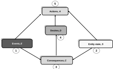
The meta – matrix of our model is a 5×5 matrix of causality, influence, correlation, etc. graphs between previously identified sets E (events), S (entity state), C (consequences), D (desires) Desires, D Entity state, S Events, E Consequences, C Actions, A 1 2 3 4 5
and A (actions) as shown by the following Figure 5 where blank entries mean no direct influence of the corresponding sets.
E S C D A E E-E graph E-C graph S S-S graph S-C graph C C-C graph C-D graph D D-D graph A A-E graph A-S graph A-A graph
Figure 5. Meta-matrix of the model
These graphs are presented in the following points.
Events graph (E-E graph): this graph defines
causal relationships that may exist between events; to identify these relationships one must answer questions such as "which event may lead to which one?" For instance an earthquake may cause a tsunami or stones fall in mountains regions.
State graph (S-S graph) represents potential
influence that may exist between the variables defining the state of the entity.
Consequences graph (C-C graph) defines
relationships between consequences. For instance, human consequences during an
earthquake may be decomposed into economic consequences, infrastructures consequences, cultural consequences, etc. To define this graph one can use a bottom up analysis, going from a particular consequence and identifying all the consequences that lead to it.
Desires graph (D-D graph) is similar to
consequences graph.
Actions graph (A-A graph): this graph defines
how one action may influence another one or how the success of an action may depend on another one.
Events-Consequences graph (E-C graph) defines
how uncontrollable variables representing events will impact the consequences.
Sate-Consequences graph (S-C graph): this
graph signifies that the importance of consequences depend on the state of the entity in terms of vulnerability or resiliency.
Consequences-Desires graph (C-D graph) is
straightforward as desires are defined as conditions or constraints over consequences.
Actions-Events graph (A-E graph): this graph
represents the risk prevention actions as for some events there may exist actions that reduce their likelihood.
Actions-State graph (A-S graph) describes how
some actions influence the state of the entity; indeed this graph represents the risk mitigation actions effects.
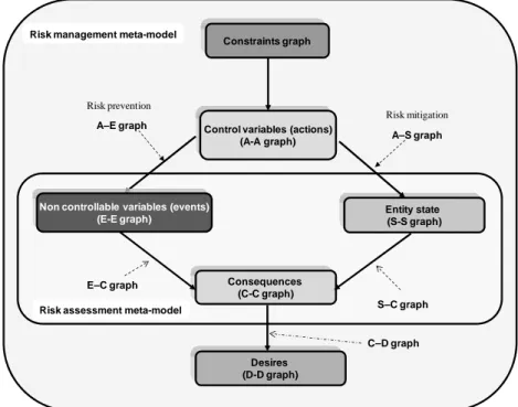
Control variables (actions) (A-A graph) Desires (D-D graph) Constraints graph Consequences (C-C graph) Entity state (S-S graph) Risk mitigation Risk prevention
Risk assessment meta-model Risk management meta-model
Non controllable variables (events) (E-E graph) A–E graph A–S graph E–C graph S–C graph C–D graph
From the meta-matrix, defining a meta-model in terms of meta-Bayesian network is straightforward and is given by Figure 6 where we add a constraints graph that has an influence on actions in order to take into account unavoidable resources limitation and other physical and feasibility requirements for actions. Of course when facing a real problem, the meta-model of Figure 6 must be instantiated with knowledgeable variables to obtain a real Bayesian network to support making decision. A Bayesian network is constituted by two components: its structure that is directly given by Figure 6 and its parameters that are conditional probability tables (in the case where nodes take discrete modalities) or conditional distribution functions (for continuous nodes) as well as a priori distributions for nodes that do not have parents. Thus, in front of a real problem, the analyst has to make hypothesis concerning the nature of nodes. In this paper we consider only discrete nodes because Bayesian networks with discrete nodes are those easily handle by existing algorithms for learning and inference (see [9, 11]) and also because the framework we are building will be dedicated to high level managers that reason most of the time in terms of macro variables and tendency rather than precise numbers. Another reason for adopting discrete nodes is that most of the time experts’ knowledge is required to elicit conditional probability distribution and these experts express their knowledge fuzzily which fuzzy measures can be translated to probability by appropriate approaches such as pignistic probability approach, see [15]. So, all continuous variables will be discretized using possibly fuzzy discretization.
2.3. Usage of the model
The overall model can be used in two senses: deductive or inductive. In deductive sense, by specifying some local evidence in the model, one can propagate it using inference algorithms of Baysian networks to estimate the resultant risk Rd(X) on each desire d and then aggregate
them by means of equation (6) to obtain the overall resultant risk R(X). In inductive sense, by giving some requirements concerning acceptable risk for each desire, one can back propagate this information to determine the most appropriate actions to set up. One must notice that this model can be used by portion in the sense that
the user can be interested in only a subset of variables and do the propagations processes.
3. Illustrative Example
To illustrate the approach presented so far, we consider a problem of developing a model that can be used by authorities of a country or a region (that may face an earthquake events) to support making sound decisions before, during and after an earthquake. This is a preliminary analysis which purpose is to show that steps and tools presented previously can be used effectively; variables and their categories that will be presented in the following paragraphs are developed by the author as a first attempt. The methodology presented is obviously multidisciplinary, be it to identify relevant variables and relationships or to characterize their strength by conditional probabilities. In the following paragraphs, we will apply the steps described on the flow chart of Figure 3 to identify some variables that can be used to assess or manage risk related to an earthquake event; we do not pretend to exhaustiveness and the adopted clustering in terms of consequences, state of the system, actions or desires may raise objections but we do think that this study can easily be adapted by a multidisciplinary team for a real world project.
3.1 Variables and relationships
3.1.1. Events. As it is shown on Figure 3, the first step in risk management process we have proposed is to identify potential adverse events; here the main event is the earthquake and subsidiary it can cause others events such as a tsunami. Earthquake is the principal event and it can be characterized in the framework of a Bayesian network by a discrete variable which modalities or status can be determined using Richter scale for instance. A tsunami can result from an earthquake so that earthquake is a causal event for a tsunami in the structure of E-E graph. Tsunami can be evaluated by a binary modalities (Yes/No) or by more modalities such as Very Huge/Huge/Medium/Small. These later characterization may result from a (fuzzy) discretization of a physical parameter such as the energy or the mass of water displaced by the tsunami.
3.1.2. Entity state characterization. The second step of the chart on Figure 3 is to characterize the state of the entity (here the strength and weakness of the region under
consideration with regard to earthquake events and other possible conditions). We consider that the state of the system can be described by the following variables that obviously will impact on the consequences of an earthquake in a region. Of course one can imagine many other variables and the process of identifying these variables in a real world application will certainly be carried up by a multidisciplinary team.
Population awareness of the phenomenon: this is a qualitative appreciation of how well the concerned population know that an earthquake can occur in the region; indeed a well prepared population will probably adopt a good behaviour during an earthquake than a non prepared one. In the framework of Bayesian networks, this variable is a discrete variable that can be evaluated on a Yes/No scale or a more elaborated scale such as Good/Medium/Low.
Infrastructure conditions: a region where infrastructures (buildings, roads, dams, etc.) are built when respecting anti-seismic norms will probably resist better during an earthquake than a region that does not respect these norms. This variable may be hierarchically decomposed into other variables (age of the infrastructure, usage of the infrastructure, etc.) which modalities are easier to define.
Emergency systems: this variable describes the quantity and qualities of resources developed by the region authorities to monitor adverse events (network of sensors to detect tectonic movements, geographic information systems, communication systems, etc.) and to efficiently react during an event (emergency equipment, quality and quantity of emergency trained agents, etc.). As for infrastructure conditions variable, this one also can be considered as a macro-variable that can be decomposed into many more measurable variables.
Education level: a well educated population will be more receptive to prescribed behaviour during an earthquake than a non educated one. This variable in terms of Bayesian network will be a parent of the variable population awareness and can be evaluated on a discrete scale such High/Medium/Low that could be a fuzzy discretization of a continuous variable such as the proportion of the population that earn a certain degree for instance.
3.1.3. Consequences characterization. Once events and the state of the system are defined, one can consider identifying consequences that
may occur in response to an event. The consequences of an earthquake event are certainly multiples; here is an attempt to categorize them in terms of economic, social, infrastructures and environmental consequences. 3.1.3.1. Economic consequences: economic consequences consist in immediate consequences and long term consequences; here is a non exhaustive list.
Loss of jobs and know how: this can be considered to be a mean/long term consequence; after an earthquake many people will probably loose their jobs because of damage caused to their working infrastructures and lives loss will result in loss of know how in long term. This is a macro-variable.
Macro-economic consequences: destruction of industrial infrastructures and others will lead to negative macro-economic consequences; this variable obviously will be decomposed into other variables in real case and can be considered to be a descendant of the previous variable Loss of jobs and know how.
Relocation (of population) cost: this is an immediate consequence that will be influenced by some variables related to emergency systems and infrastructure conditions of the state of the entity and though it is naturally a continuous variables, it will be discretized in
natural language (Very high/High/Medium/Low for instance) for sake
of communication.
Evacuation (of population) cost: this is also an immediate consequence as the previous one and will be characterized almost in the same way, etc.
3.1.3.2. Social consequences: as economic consequences, one can imagine many social consequences such as those listed in the following.
Lives loss: this is normally a continuous variable that will be fuzzily discretized to have a linguistic scale. It will depend on some state of the entity variables and other consequences (consequences on buildings for instance).
Impact on the revenue: economic consequences such as jobs loss will lead to a reduction in revenue of the population that will increase social dependency for instance.
Impact on the social dependency: as stated in the previous point, reduction in the revenue may increase social dependency among the population.
Impact on education level: lives loss, revenue reduction and social dependency may lead to a negative impact on the education level.
Post event social consequences: these consequences could consist in changes in cultural habits (migration of people from rural area to towns that will raise some problem such as criminality) or an impact on the structure of the population (reduction of active members of the population), etc.
3.1.3.3. Infrastructure consequences.
Consequences on buildings: damages caused to building will depend on the intensity of the earthquake as well as the nature of the buildings (are the buildings constructed when respecting anti-seismic norms or not?) and they will impact on lives loss that will depend on the usage of the building (office, home, industrial building, etc.). These consequences can be evaluated over scales defined by existing norms such as that of Eurocode (see for instance [24]). Loss of energy infrastructures: this variable, that will be a descendant of variables such as dams, power plants, power lines, etc., will influence socioeconomic consequences variables such as macro-economic consequences, jobs loss, etc. In terms of Bayesian networks it will be evaluated over a discrete scale.
Loss of communication resources: the loss of communication infrastructures such as roads, bridges, airports, ports or electronic communication infrastructures will result in negative socioeconomic consequences such as goods getting expensive or jobs loss because of lake of row materials to run industries.
3.1.4. Environmental consequences. Some resulted events from an earthquake such as tsunami, floods or fire or consequences such as explosion of chemical plants or nuclear power plants for instance may conduce to negative consequences on the environmental resources; here is some of those potential consequences. Impact on water resources: contamination of rivers and underground water by dangerous products from an exploded chemical or nuclear plants. This variable will have an impact on economic and social consequences mainly in the rural area and can be considered as a macro-variable that can be decomposed into more measurable variables.
Impact on agriculture resources: flooded area may become impracticable for agriculture or crops may be destroyed by fire, floods or a
tsunami. This impact will ultimately affect economic and social consequences.
Climate consequences: destruction of forests by fire resulted from an earthquake or by a tsunami can have a long term consequences on the climate of the considered region that in return will impact on long term social and economic consequences.
3.1.5. Actions identification. According to the nature of the adverse event (an earthquake that is a matter of nature), only risk mitigation actions can be implemented. These actions will act on some of the variables of the state of the entity to reduce negative consequences. Given former identified variables of the state of the system, here are some actions that can be imagined. Prepare population, this action could take different forms: educate the population; inform and train population to have a good behaviour in the case of an earthquake.
Set up and organize emergency systems: create a network of sensors to pre-detect an earthquake event in order to alert population by different media; train qualitatively and quantitatively agents for reactive response; equip emergency agencies with good materials, etc.
Prepare after event: constitute a fund or subscribe insurance to face after events problems. Take legislative decisions: vote laws and norms to be respected when constructing some infrastructures (buildings, dames, power plants, roads, bridges, etc.); force individuals and companies to contract risk insurances, etc. 3.1.6. Desires formulation. Risk management desires here will consist in implementing actions in order to reduce the level of some negative consequences so that desires may be defined by thresholds on consequences level or constraints satisfaction by some consequences: have low level lives loss, prevent infrastructures collapse, prevent occurrence of hunger, etc.
3.1.7. Constraints specification. Constraints may be subdivided into different fields such as those given below.
Financial constraints: the considered country or region may face serious financial resources limitation in order to undertake actions defined previously.
Technical constraints: the region or country may lack technical skills to train emergency agents; to construct and organize an efficiency emergency system; to design and construct
adequate infrastructures. These constraints are directly influenced by financial constraints that constitute then a parent node in the framework of Bayesian network.
Geographic constraints: the accessibility of a region that face a natural disaster by emergency resources may be very difficult (mountains region for instance).
Period of the day: according to the period of the day an earthquake takes place it will be more or less easy to organize emergency systems and rescue people. This variable will be evaluated naturally by modalities such as morning, afternoon, night, etc. in a Bayesian network.
3.2 An instance of the model
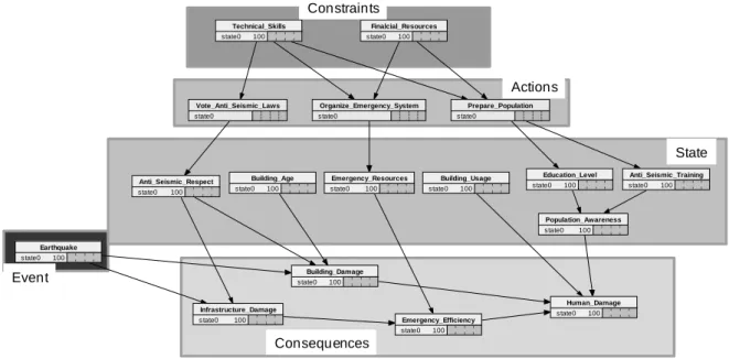
Once variables are identified and their relationships sketched, one can consider building the entire model. This can be done by implementing existing Bayesian network learning and inference algorithms [9, 11] to construct one’s own decision support system or one can use existing decision support software based on Bayesian network technology such as that of [8, 13], the principal ones in our knowledge. Figure 7 shows an extract of a model (built using Nertica) that could be set up to support decision making and planning regarding risk related to an earthquake event in a building; the focused consequence in this extracted model is human damage. Notice that variables in this model can be considered as macro variables that can be decomposed into more elementary variables depending on the level of abstraction decision makers accept. We
did not find it necessary to consider specifying modalities of variables nor conditional probability tables as this is just an illustration of what can be obtained as structure of a risk management decision model in a particular case using the developed approach. When necessary, by using a team of experts, specification of these parameters can be done
without major difficulties and value nodes can be added so that one can optimize or prioritize actions by simulation.
4. Conclusion
A generic framework and model to support managing risks related to variability and fuzzy uncertainties has been considered in this paper. A procedure based on questions – responses has been proposed to identify all the variables (risk factors, state of the entity under consideration, possible consequences, possible risk reduction actions) impacting decision-making process. Then, a meta-matrix analysis is proposed to identify relationships between these variables and to assess their strength. As the main purpose of the established model is to aid decision maker making inductive and deductive analysis for pre-active, reactive, and proactive decisions making, this model must be able to propagate local evidence through the variables to assess or identify most suitable status of some interested variables. To respond to this later concern, Bayesian networks and influence diagrams have been chosen as the underlying mathematical tools of the
Finalcial_Resources state0 100 Technical_Skills state0 100 Vote_Anti_Seismic_Laws state0 Organize_Emergency_System state0 Prepare_Population state0 Education_Level state0 100 Anti_Seismic_Training state0 100 Population_Awareness state0 100 Building_Usage state0 100 Emergency_Resources state0 100 Building_Age state0 100 Anti_Seismic_Respect state0 100 Human_Damage state0 100 Infrastructure_Damage state0 100 Building_Damage state0 100 Earthquake state0 100 Emergency_Efficiency state0 100 Consequences Actions Constraints State Event
established framework. Fuzzy integral, namely Choquet integral (that permits to take into account interactions between aggregated parameters) is used for aggregation purpose in order to present managers with concise information. Though the illustrative example we have presented concerns decision-making in relation with a natural disaster (earthquake), the established framework is much general to be applied or adapted for risk management in other domains such supply chain, food industry, banking and finance, engineering, medical to name few. Future works will focus on applying this approach to a real world problem and developing useful computers applications based on this framework.
REFERENCES
1. AVEN, T., Reliability and Risk Analysis, 1st Ed. Elsevier Applied Science, 1992. 2. BAYES, T., Towards Solving a Problem
in the Doctrine of Chances, Biometrica (46), 1958, pp. 293-298 (reprinted from an original paper of 1763).
3. GRABISCH, M., Fuzzy Integral in Multicriteria Decision Making, Fuzzy Sets & Systems 69, 1995, pp. 279-298. 4. GRABISCH, M., The Application of
Fuzzy Integrals in Multicriteria Decision Making, European J. of Operational Research 89, 1996, pp. 445-456.
5. GRABISCH, M., K-Order Additive Discrete Fuzzy Measures and Their Representation, Fuzzy Sets & Systems 92, 1997, pp. 167-189.
6. HOWARD, R. A., MATHESON, J. E., Influence Diagrams, in The principles and Applications of Decision Analysis, R. A. Howard and J.E. Matheson (Eds) (2), 1984, pp. 719-762.
7. HM TREASURY, The Orange Book. Management of Risk - Principles and Concepts, Crown, 2004.
8. Hugin Expert, http://www.hugin.com/ 9. JENSEN, F. V., Bayesian Networks and
Decision Graphs, Springer, 2001.
10. MAGNE, L., D. VASSEUR, Risques Industriels. Complexité, Incertitude et Decision: une approche interdisciplinaire, (in french), Lavoisier, 2006.
11. MURPHY, K. P., Dynamic Bayesian Networks: Representation, Inference and Learning, Ph.D. Thesis, University of California, Berkeley, 2002.
12. NAÏM, P., P.-H. WUILLEMIN, P. LERAY, O. POURRET, A. BECKER, Réseaux bayésiens (in french), Eyrolles, 2004. 13. Netica, http://www.norsys.com/
14. PEARL, J., Probabilistic Reasoning in Intelligent Systems, Morgan Kaufmann, 1988.
15. SMETS, P., KENNES, R., The Transferable Belief Model, Artificial Intelligence, vol. 66, 1994, pp. 191-243. 16. SINGPURWALLA, N. D., Reliability and
Risk: A Bayesian Perspective, John Wiley & Sons, 2006.
17. STAMATIS, D. H., Failure Mode and Effect Analysis - FMEA from Theory to Execution, ASQC Quality press, 1995. 18. SUTTON, I. S., Process Reliability and
Risk Management, 1st Ed. Van Nostrand Reinhold, 1992.
19. TCHANGANI, A. P., Reliability Analysis using Bayesian Networks, Studies in Informatics & Control Journal vol. 10(3) , 2001, pp. 181-188.
20. TCHANGANI, A. P., D. Noyes, Modelling Dynamic Reliability using Dynamic Bayesian Networks, European Journal of Automation, vol. 40(8) , 2006, pp. 911-935.
21. TERANO, T., K. ASAI, M. SUGENO, Fuzzy Systems Theory and Its Applications, Academic Press, 1987.
22. THORAVAL, P.-Y., Le dispositif de Bâle II: rôle et mise en oeuvre du pilier 2, Revue de la stabilité financière (9), Banque de France, 2006, pp. 125-132, (in french). 23. WALD, A., Statistical Decision
Functions, New York: Wiley, 1950.
24. Working Group Macroseismic Scales, European Macroseismic Scale 1998 EMS-98, Cahiers du Centre Européen du Géodynamique et de Sismologie (15), Edition Conseil de l'Europe, 1998.