O
pen
A
rchive
T
OULOUSE
A
rchive
O
uverte (
OATAO
)
OATAO is an open access repository that collects the work of Toulouse researchers and
makes it freely available over the web where possible.
This is an author-deposited version published in :
http://oatao.univ-toulouse.fr/
Eprints ID : 12509
The contribution was presented at PDPTA 2013 :
http://www.worldacademyofscience.org/worldcomp13/ws/conferences/pdpta13.html
Official URL:
http://worldcomp-proceedings.com/proc/p2013/PDP.html
To cite this version :
Mayap Kamga, Christine Larissa and Hagimont, Daniel
Virtual processor frequency emulation. (2013) In: 19th International Conference
on Parallel and Distributed Processing Techniques and Applications (PDPTA
2013) held as part of WORLDCOMP'13, 22 July 2013 - 25 July 2013 (Las Vegas,
United States).
Any correspondance concerning this service should be sent to the repository
administrator:
staff-oatao@listes-diff.inp-toulouse.fr
Virtual processor frequency emulation
Christine Mayap and Daniel Hagimont
Institut National Polytechnique de Toulouse ENSEEIHT, 2 rue Charles Camichel
31000 Toulouse, France Email: hagimont@enseeiht.fr
Abstract—Nowadays, virtualization is present in almost all computing infrastructures. Thanks to VM migration and server consolidation, virtualization helps in reducing power consumption in distributed environments. On another side, Dynamic Voltage and Frequency Scaling (DVFS) allows servers to dynamically modify the processor frequency (according to the CPU load) in order to achieve less energy consumption. We observe that while DVFS is widely used, it still generates a waste of energy. By default and thanks to the ondemand governor, it scales up or down the processor frequency according to the current load and the different predefined threshold (up and down). However, DVFS frequency scaling policies are based on advertised processor frequencies, i.e. the set of frequencies constitutes a discrete range of frequencies. The frequency required for a given load will be set to a frequency higher than necessary; which leads to an energy waste. In this paper, we propose a way to emulate a precise CPU frequency thanks to the DVFS management in virtualized environments. We implemented and evaluated our prototype in the Xen hypervisor.
Keywords—DVFS, frequency, emulation.
I. INTRODUCTION
Nowadays, cloud computing is one of the widely used IT solutions for distributed services. Almost 70% of companies are interested in it and 40% of them plan to adopt it within one year [1]. Cloud computing can be defined as a way of sharing hardware or/and software resources with clients according to their needs. The idea of cloud computing is to simulate an unlimited set of resources for users and to guarantee a good Quality of Service(QoS), while optimizing all relevant costs [2].
Cloud computing mainly relies on virtualization. Virtualization consists of providing concurrent and interactive access to hardware devices. Thanks to his live migration properties, it is possible to migrate applications on a few number of computers, while ensuring good QoS and security isolation. This advantage is highly exploited by cloud computing to effectively manage energy consumption and to efficiently manage resources [3].
Recent advances in hardware design have made it possible to decrease energy consumption of computer systems through Dynamic voltage and frequency scaling (DVFS) [4]. DVFS is a hardware technology used to dynamically scale up or down the processor frequency according to the governor policy and the workload demand.
Knowing that, the processor power consumption is related to the frequency processor and its voltage [5], increasing or decreasing processor frequency will influence the general power consumption of a system. In this context, the choice of the processor frequency is of great importance.
Furthermore, DVFS aims at setting the CPU frequency to the first available one capable of satisfying the current load to avoid wastage. However, there may be situations where the selected frequency is still the subject of wastage because it is higher than the required frequency.
In this paper, we explore and propose a way to emulate a precise desired processor frequency in a virtualized and single-core environment. After presenting the context and the motivation of our work in section 2, we will describe our contributions in section 3. In section 4, we present experiments to validate our proposal. After a review of related works in section 5, we conclude the article in Section 6.
II. CONTEXT AND MOTIVATION
In this section, we present some concepts of virtualization, DVFS and how this later is applied in virtualized systems.
A. Context
1) Virtualization: According to a general observation, the
rate of server utilization was around 20% [6]. Thanks to virtualization, the rate has increased and allows efficient server utilization. Indeed, virtualization is a software-based solu-tion for building and running simultaneously many operating systems (called guest OS or Virtual Machine) on top of a ”classic” OS (called host OS). A special application, named
Virtual Machine Monitor (VMM) or hypervisor emulates the
underlying hardware and interprets communications between guests OS and devices.
Among existing virtualization technologies, we adopt
par-avirtualizationas the base of our experience. With
paravirtu-alization, the VMM is placed between the hardware and the host OS. Guest OS is modified to use optimized instructions (named hypercall ) from VMM to access hardware.
Paravirtualization is used because of its good VM performance and its implementation on all types of processors. In fact, with full virtualization, VM performance is more than 30% degraded [7]. Meanwhile Hardware-assisted
performance of guest OS are close-to-native performance. Paravirtualization is highly adopted and vulgarized by Xen [8] and VMWare ESX Server [9]. In this context, our work is based on Xen platform because it is prevalent in many computing infrastructures, as well as in the vast majority of our previous work.
2) Dynamic Voltage and Frequency Scaling (DVFS):
To-day, all processors integrate dynamic frequency/voltage scaling to adjust frequency/voltage during runtime. The decision to change the frequency is commanded by the current processor’s
governor. Each governor has its own strategy to perform
frequency scale. According to the configured policy, governor can decide to scale processor speed to a specific frequency, the highest, or the lowest frequency.
Several governors are implemented inside the Linux kernel.
Ondemand governor changes frequency depending on CPU
utilization. It changes frequency from the lowest (whenever CPU utilization is less than a predefined (low therehold) to the highest and vice-versa. Performance governor always keeps the frequency at the highest value while slowest CPU speed is always set by powersave governor. Conservative governor decreases or increases frequency step-by-step through a range of frequency values supported by the hardware. Userspace governor allows user to manually set processor frequency [10]. In order to control CPU frequency, governors use an un-derlying subsystem inside the kernel called cpufreqq [11]. Cpufreq provides a set of modularized interfaces to allow changing CPU frequency. Cpufreq, in turn, relies on CPU-specific drivers to execute requests from governors.
As aforementioned, effectively usage of DVFS brings the advantage of reducing power consumption by lowering proces-sor frequency. Moreover, almost all computing infrastructures possess multi-core and high frequency processors. Thus, the benefit from using DVFS has been realized and achieved in many different systems.
The next section describes the motivation of this work.
B. Motivation
During the last decade, several efforts have been made in order to find an efficient trade-off between energy consump-tion/resources management and applications performance. Most of them relies on DVFS, and are highly explored due to the advent of new modern powerful processors integrating this technology.
According to the ondemand governor (the default gov-ernor policy implemented by DVFS), the CPU frequency is dynamically changed depending on the CPU utilisation. With this governor, the highest available processor frequency is set when the CPU load is greater than a predefined threshold (up threshold). When the load decreases below the threshold, the processor frequency is decreased step by step until the one capable of satisfying the current process load is found.
However, in most CPUs, the DVFS technology provides a reduced number of frequency levels (in the order of 5) [12]. This configuration might not be enough for some experiments.
Suppose a virtualized muti-core processor Intel(R) Xeon(R) E5520 with 2.261 GHz and the DVFS technology enable. Consider its six frequencies levels distributed as fol-lows: 1.596 GHz, 1.729 GHz, 1.862 Ghz, 1.995 Ghz, 2.128 GHz and 2.261 GHz. Assume the host OS with a global load which needs 1.9285 Ghz to be satisfied. Knowing that the computation of the best execution time of an application is made on a basis of the maximum frequency of a processor, scheduling it with a lower frequency would end up with a lower than expected performance. From the SLA point of view and because of the non-existence of the expected frequency, the ondemand governor will set the CPU frequency to the first one, higher that the required frequency, capable of satisfying the current load. Precisely in our example, the ondemand governor will set the processor frequency to 1.995 GHz.
However, it would be more beneficial in terms of energy to assign to the processor the exact required frequency. Indeed, the DVFS technology consists of concurrently lowering the CPU voltage and the CPU frequency. By lowering them, the current total energy consumption of the system is globally de-creased [13]. To improve this well-known energy management, we will realise some adjustments on the DVFS technology. Hence, instead of setting the CPU frequency to the first higher available frequency, we decided to emulate some of the non-existent CPU frequency according to the system needs.
Concretely, emulating a CPU frequency, in our work, con-sists of executing the processor successively on the available frequencies around the desired CPU frequency. Our emulation process is essentially based on the conventional operation of the DVFS. The use of the DVFS possesses as asset the fact of generating no overhead while switching between frequencies because it has been done in the hardware.
The next section describes our contributions.
III. CONTRIBUTION
As previously mentioned, the main idea of this paper is to emulate a CPU processor frequency based on periodic oscillations of frequencies between two levels of successive frequencies. This extension will suggest a way of decreasing power consumption in virtualized systems while keeping good VM performance. The next section will expound our approach and the implementation we made.
A. Our appraoch
Our approach is two folds: (1) To determine the exact processor frequency need by the current load and (2) to emulate it if necessary.
Let’s assume a host with several VMs running on it. Suppose that they generate a global load of Whost. Consider
that we need our CPU to be running at processor frequency of fhost to satisfy the current load (Whost). However, the desired
processor frequency fhost is not present among the available
processor frequencies of our host. This frequency need to be emulated.
A weighted average can be defined as an average in which each quantity to be averaged is assigned a weight. These weightings determine the relative importance of each quantity on the average. Weightings are the equivalent of having that
many similar items with the same value involved in the average. Indeed, the emulation of CPU processor is based on weighted average of CPU frequency around the frequency to emulate. Although it is possible to determine in advance the neighboring processor frequencies, the computation of the execution time for each of them is not realistic.
Firstly, we need to determine the required frequency and later the both frequencies around the desired one. Assume that fhighand flow are the frequency above and below the desired
frequency respectively. To emulate fhost, we need to compute
our load during thighat fhighand during tlow at flowso that
the required frequency fhost is the weighted-average of fhigh
with thigh as weight and flow with tlow as weight. It means
that:
fhost=
(fhigh×thigh) + (flow×tlow)
thigh+ tlow
(1) Unfortunately, it is not possible to determine beforehand the exact execution times allowing to fulfill the equation 1. Instead of considering thighand tlowas the execution time, we
exploited it as the occurrence count. Meaning that to emulate fhost, the processor needs to be executed thightimes in higher
frequency fhigh and tlow times in lower frequency flow.
It is important to note that, the real execution time at each processor frequency level can be computed as follows: N umberOccur × T ickDuration . Where N umberOccur represents either thighor tlowand T ickDuration the duration
of each tick of reconfiguration.
To validate this assumption, let’s consider the small exam-ple of II-B. By executing our processor, once on the lower frequency (that means at 1.862 Ghz) and once on the higher frequency (that means 1.995 Ghz), we will obtain the required frequency (1.9285 Ghz).
It means that: fhost = 1.995×1+1.862×11+1 = 1.9285
As aforementioned, the number of executions at each processor frequency cannot be known at the beginning of the experiments. It must be dynamically computed.
The next section presents our implementation.
B. Implementation
In this section, we address the design and the implementa-tion choices of our frequency emulator, and the condiimplementa-tions of his exploitation.
Our implementation is two folds: (1) checking the appropri-ate processor frequency for the current load and (2) emulating If it is not existing.
1) Appropriate processor frequency: By default DVFS
advertises a discrete range of processor frequencies. It means that, only a fixed and predefined number of processor frequen-cies are available.
To fulfill the first aspect of our work (determine the adequate frequency), we assume that, on each processor, it is possible to have a continuous range of frequencies. Know-ing that the difference between two successive frequencies is practically identical, we virtually subdivided them into 3 (value obtained thanks to analysis and successive experiments). Indeed, this subdivision allowed the obtaining of the more
moved closer frequencies. This nearness at the level of the frequencies so allowed to satisfy at best the processor’s loads. Assuming that the frequency range is now continuous, it is then always possible to have a precise processor frequency for a given load. The return of the suitable processor frequency is made according to the frequency ratio presented in our proposal in [8].
Indeed, at each tick of the scheduler, a monitoring module gathers the current CPU load of each VM. It then aggregates the total Absolute load of all the VM and computes the new processor frequency and the frequencies surrounding it, as depicted in the algorithm below (Listing 1) where
• LFreq[]: represents a table of 3 processor frequencies
classified as follows: the required frequency and the surrounding ones (higher and lower respectively)
• VFreq: value obtained after the division of the interval
between consecutive frequencies by 3. It is used to obtain some virtual processor frequencies.
• Freq[]: represents the available processor frequencies.
The table is sorted in descending order.
We iterate on the processor frequencies (line 2). Following our assumption regarding frequencies (it will be validated in section IV-B1), we compute for each frequency the frequency ratio (line 3) and check if the computing capacity of the processor at that frequency can absorb the current absolute load (line 6). If the current frequency can not satisfy the load, we iterate on virtual processor frequencies (line 22 to line 29). 1 void computeNewFreq(int LFreq[], int VFreq) {
2 for (i=1; i<=fmin; i++) {
3 int ratio = Freq[i]/Freq[1];
4 int NFreq;
5
6 if(ratio * 100 < Absolute_load){
7 if ((i == 1) || (i == fmin){
8 LFreq[0] = LFreq[1] = LFreq[2] = Freq[i];
9 }
10 else{
11 LFreq[0]= Freq[i] + VFreq;
12 LFreq[1]= Freq[i-1];
13 LFreq[2]= Freq[i];
14 }
15 }
16 else{
17 NFreq= Freq[i] - VFreq;
18 LFreq[1] = Freq[i];
19 LFreq[2] = Freq[i+1];
20 ratio = NFreq/Freq[1];
21
22 while (ratio * 100 > ratio){
23 if (NFreq != Freq[i+1]){ 24 NFreq -= VFreq; 25 ratio = NFreq/Freq[1]; 26 } 27 else 28 break; 29 } 30 if (ratio * 100 < Absolute_load){ 31 NFreq += VFreq; 32 if (NFreq == Freq[i]){
33 LFreq[1] = LFreq[2] = Freq[i];
34 }
35 LFreq[0] = NFreq;
36 }
37 }
38 }
Listing 1. Algorithm for computing the adequate processor frequency and the surrounding frequencies
By the end of the algorithm, if the required frequency is not among the known frequency of the processor, it is immediately emulated.
2) Processor frequency emulation: The emulation is based
on the cumulative functions principle. It is convenient to describe data flows by means of the cumulative function f(t), defined as the number of elements seen on the flow in time interval [0, t]. By convention, we take f(0) = 0, unless otherwise specified. Function f is always wide-sense increasing, it means that f(s) ≤ f (t) for all s ≤ t.
Suppose 2 wide-sense increasing functions f and g, the notation f+ g denotes the point-wise sum of functions f and g.
(f + g)(t) = f (t) + g(t) (2) Notation f ≤(=, ≥) g means that f (t) ≤ (=, ≥) g(t) for all t [14].
To exploit this notion, we defined 3 cumulative frequency functions: CumFhigh(t), CumFlow(t) and CumFhost(t).
Where CumFhigh(t), CumFlow(t) and CumFhost(t)
repre-sent the functions for the higher processor frequency , the lower and the required processor frequency respectively. In our case, we defined the cumulative frequency corresponding to a particular value as the sum of all the frequencies up to and including that value. Meaning that: CumFhigh(t) =
Pt
k=0fhigh.
At each tick of the scheduler and for each frequency involved (including the emulated frequency) in the emula-tion of the frequency, we compute its cumulative frequency (Listing 2). The computation of each cumulative frequency is executed as follow:
• Initially, the cumulative frequencies functions are equal to zero (their initial value). This value is reini-tialized when the current load need a different fre-quency or when the current one is already emulated (line 17),
• At each tick, the cumulative frequency of the emulated frequency (CumFhost(t)) is incremented by its value:
CumFhost(t) + = fhost (line 7 and line13),
• At each tick, only one frequency is set (either fhigh
or flow). The choice of the frequency is carried out as
follows:
◦ The sum of CumFhigh(t) and CumFlow is
computed according to the equation 2 and the result is compared to CumFhost(t) (line 3),
◦ If the sum is lower than CumFhost(t), then
the processor frequency is set to fhigh during
the next quantum (line 6),
◦ Else, if the sum is higher than CumFhost, the
processor frequency is set to flow during the
next quantum (line 12),
◦ If both are equal, the desired frequency was emulated and the different cumulative frequen-cies are reinitialized (line 17).
Through these iterations and these oscillations, we managed to emulate our desired frequency. It should be mentioned that, the emulated frequency and the neighboring frequencies are obtained with the algorithm presented in Listing 1.These later (table LFreq[]) are passed as a parameter to the algorithm below.
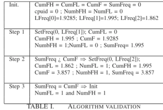
For instance, if we consider our example of section II-B, the goal was to emulate a processor frequency of 1.9285 Ghz. The surrounding frequencies are 1.995 Ghz and 1.862 Ghz. The execution of the algorithm of Listing 2 is as follows (Table I ):
Init. CumFH = CumFL = CumF = SumFreq = 0 cpuid = 0 ; NumbFH = NumFL = 0
LFreq[0]=1.9285; LFreq[1]=1.995; LFreq[2]=1.862 Step 1 SetFreq(0, LFreq[1]); CumFL = 0
CumFH = 1.995 ; CumF = 1.9285 NumbFH = 1;NumFL = 0 ; SumFreq= 1.995 Step 2 SumFreq ¿ CumF ⇒ SetFreq(0, LFreq[2]);
CumFL = 1.862 ; NumFL = 1; CumFH = 1.995 CumF = 3.857 ; NumbFH = 1, SumFreq = 3.857 Step 3 SumFreq = CumF ⇒ Init
NumFL = 1 and NumFH = 1
TABLE I. ALGORITHM VALIDATION
This execution validates the number of time needed to emulate 1.9285 Ghz as presented in section III-A.
1 void EmulateFrequency(int LFreq[], int CumFH,int CumFL, int CumF,int cpuid) {
2 int SumFreq;
3 SumFreq = CumFH + CumFL;
4 5 if (SumFreq < CumF){ 6 SetFreq(cpuid,LFreq[1]); 7 CumF += LFreq[0]; 8 CumFH += LFreq[1]; 9 } 10 else{ 11 if (SumFreq > CumF){ 12 SetFreq(cpuid,LFreq[2]); 13 CumF += LFreq[0]; 14 CumFL += LFreq[2]; 15 } 16 else{
17 CumF = CumFH = CumFL = 0;
18 }
19 }
20 }
Listing 2. Emulate processor frequency
During this execution, we remind that there is a trigger in charge of the computation of the absolute load and the notification of the current desired frequency. This situation also leads to a reinitialization of all the cumulative frequencies value.
The next section presents some experiments to validate our proposal.
IV. VERIFICATION OF OUR PROPOSAL
We previously presented our approach and its implementa-tion in the default Xen credit scheduler. In this secimplementa-tion, we will present the experiment environment, the application scenario and some experiments to validate our proposition.
A. Experiment environment and scenario
Our experiments were performed on a DELL Optiplex 755, with an Intel Core 2 Duo 2.66GHz with 4G RAM. We run a Linux Debian Squeeze (with the 2.6.32.27 kernel) in a single processor mode. The Xen hypervisor (in his 4.1.2 version) is used as virtualization solution. The evaluation described below was performed with an application which computes an approximation of π. This application is called π-app. In this scenario, we aim at measuring an execution time.
B. Verification
1) Proportionality: In our validation, we rely on one main
assumption: proportionality of frequency and performance. This property means that if we modify the frequency of the processor, the impact on performance is proportional to the change of the frequency.
This proportionality is defined by: Fi
Fmax
= Tmax Ti
(3) which means that if we decrease the frequency from Fmax down to Fi, the execution time will proportionally
increase from Tmax to Ti. For instance, if Fmax is 3000 and
Fi is 1500, the frequency ratio is 0.5 which means that the
processor is running 50% slower at Ficompared to Fmax. So
if we consider an application that runs in 10 mn at Fmax, the
same application will be completed at 10
0.5 = 20mn at Fi.
To validate this proportionality rule, we conducted the following experiment. We ran different π-app workloads at different processor frequencies and measured the execution times, allowing us to verify the proportionality of frequency ratios and execution time ratios. Figure 1 gives some of the results we obtained, which shows that frequency ratios and execution time ratios are very close, as assumed in equation 3.
Fig. 1. Proportionality of frequency and execution time
2) Validation: Our textbed advertises the following
pro-cessor frequency: 2.66GHz, 2.40GHz, 2.13GHz, 1,86GHz and 1.60GHz.
The first part of our validation consists on validate our approach of emulation. For this validation, we executed our
π-appapplication initially at 2.4 Ghz. Based on our proposal, we will execute the same computation by emulating the frequency 2.4 Ghz. We started by a well-known frequency for this
workshop, but others experiences not presented here emulate the non-existent frequency.
0 1600 1867 2133 2400 2667 0 100 200 300 400 500 0 10 20 30 40 50 60 70 80 90 100 Processour Frequency (MHz) Load (%) Processor Frequency VM
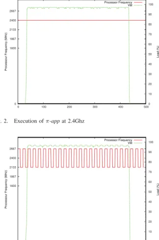
Fig. 2. Execution of π-app at 2.4Ghz
0 1600 1867 2133 2400 2667 0 100 200 300 400 500 0 10 20 30 40 50 60 70 80 90 100 Processour Frequency (MHz) Load (%) Processor Frequency VM
Fig. 3. Emulation of 2.4Ghz with oscillations
According to figure 2, the execution time of the π-app is about 410 Units. While emulating the same processor frequency, we obtained an execution time of 415 Units, as depicted by the figure 3. Based on this first use case, we can validate our approach. Furthermore, with similar experiences (not presented here), we have proved that the oscillation of the frequency in non intrusive.
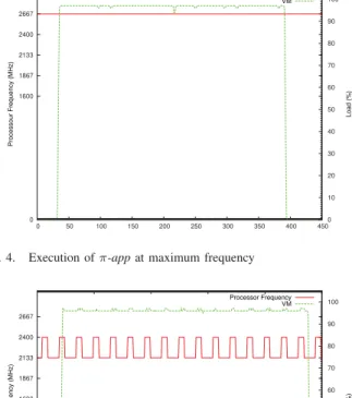
The second part consists of validating the emulation of a non-existent frequency. We executed our π-app application of the maximum frequency (figure 4 )and we recorded its execution time for future comparisons (Cf. Table II ). Then, we choose two of our virtual processor frequencies (2.222 Ghz and 2.576 GHz); we have emulated them to execute our application (respectively figure 5 and figure 6). Their execution time is used for comparison with the expected execution time according to our proportionality rule (Cf. Table II). The expected time formula is: Ti= Fmax
×Tmax
Fi
Thanks to this scenario, we can validate our implementa-tion approach. After execuimplementa-tion, we can conclude that the real execution time are almost equal to the expected time. Further evaluations are to be done in order to identify the possible weaknesses/advantages of this proposal.
0 1600 1867 2133 2400 2667 0 50 100 150 200 250 300 350 400 450 0 10 20 30 40 50 60 70 80 90 100 Processour Frequency (MHz) Load (%) Processor Frequency VM
Fig. 4. Execution of π-app at maximum frequency
0 1600 1867 2133 2400 2667 0 100 200 300 400 500 0 10 20 30 40 50 60 70 80 90 100 Processour Frequency (MHz) Load (%) Processor Frequency VM
Fig. 5. Execution of π-app at emulated frequency 2.22Ghz
V. RELATED WORKS
Numerous research projects have focused on optimization of the operating cost of data centers and/or cloud computers. Most of them concerned efficient power consumption [15]. Proposed solutions are based on either virtualization or DVFS. In virtualized environment, power reduction is made possi-ble through servers’ consolidation and live migration. Classic
0 1600 1867 2133 2400 2667 0 50 100 150 200 250 300 350 400 450 0 10 20 30 40 50 60 70 80 90 100 Processour Frequency (MHz) Load (%) Processor Frequency VM
Fig. 6. Execution of π-app at 2.578Ghz
Frequency Execution Expected time (s) (GHz) Time (s) 2.667 108.65 2.222 131.52 Ti= 2.667×108.65 2.222 = 130.41 2.578 112.79 Ti= 2.667×108.65 2.578 = 112.40
TABLE II. EXECUTION TIME RESULTS
consolidation consists on gathered multiples VMs (according to their load) on top of a reduced number of physical comput-ers [16].
In [17], Verma et al. aims at minimizing power consump-tion using consolidaconsump-tion after server workload analysis. They design two new consolidation approaches based respectively on, peak cluster load and correlation between applications before consolidating. Mueen et al. Strategy for power reduction consists in categorizing servers in pools according to their workload and usage. After categorizing, server consolidation is executed on all categories based on their utilization ratio in the data center [18].
As for the live migration, it consists of migrating a VM from a physical host to another without shutting down the VM. Korir et al [19] proposes a secure solution of power reduction based on live migration and server consolidation. Their security constraints are related to VM migration. Indeed, critical challenge of VM live migration appears when VM is still running when migration is in process. Well known attacks, such as Time-of-heck to time-of-use (TOCTTOU) [20] and replay attack, can be launched. In their solution, they design a live migration solution capable of avoiding VM to be exposed to eventual attacks.
One of the most rising approaches in power reduction is
Dynamic voltage and frequency scaling(DVFS) [21], where
voltage/frequency can be dynamically modified according to the CPU load. In [22], the authors design a new scheduling algorithm to allocate VMs in a DVFS-enabled cluster by dynamically scaling the voltage. Precisely, Laszewski et al. minimizes the voltage of each processor of physical machine by scaling down their frequency. In addition, they schedule the VMs on those lower voltage processors while avoiding to scale physical machine to high voltage.
In general, those previous approaches only are focused on well-known processor frequency. In [12], Blucher et al. suggests some approaches of the CPU performance emulator. Precisely, they propose and evaluate three approaches named as : CPU-Hogs, Fracas and CPU-Gov. CPU-Hogs consists of a CPU-burner process which burn and degrades the initial CPU processor according to a predefined percentage. CPU-Hogs has the disadvantage of being responsible for deciding when CPUs will be available for user processes. With Fracas, every decision is made by the scheduler. With Fracas, one CPU-intensive process is started on each core. Their scheduling priorities are then carefully defined so that they run for the desired fraction of time. CPU-Gov is a hardware based solution base. It consists on leveraging the hardware frequency scaling to provide emulation by switching between the two frequencies that are directly lower and higher than the requested emulate.
Although, those approaches are related to the CPU perfor-mance, they aim at emulating a predefined known processor frequency. Concretely, their goal is the answer this question: Given a CPU (characterized by its CPU performance for example), how can we emulate another CPU with a pre-cise characteristics? Their emulation is done once and ex-periments are executed on it. In our case, it consists of a real-time emulation of CPU and it constitutes a base for an energy aware resources management.
VI. CONCLUSION AND PERSPECTIVES
With the emergence of cloud computing environments, large scale hosting centers are being deployed and the energy consumption of such infrastructures has become a critical issue. In this context, two main orientations have been suc-cessfully followed for saving energy:
• Virtualization which allows to safely host several guest operating systems on the same physical machines and more importantly to migrate guest OS between machines, thus implementing server consolidation, • DVFS which allows adaptation of the processor
fre-quency according to the CPU load, thus reducing power usage.
We observe that DVFS is mainly used, but still generates a waste of energy. In fact, the DVFS frequency scaling policies are based on advertised processor frequency. By default and thanks to the ondemand governor, it scales up or down the processor frequency according to the current load and the different predefined threshold (up and down). However, the set of frequency constitutes a discrete range of frequency. In this case, the frequency required for a specific load will almost be scaled to a frequency higher than expected; which leads to a non-efficient use of energy.
In this paper, we proposed a technique which addresses this issue. With our approach, we are able to determine and allocate a more precise processor frequency according to the current load. We subdivided the interval between two frequencies of the processor into tinier virtual frequencies. This leads to simulate a continuous processor frequency range. With this configuration and the ratio proportionality rule, it is thus almost possible to set the suitable frequency for a given load. Furthermore, thanks to oscillations, made possible through the principle of cumulative frequency, between the frequencies surrounding the desired one, it was possible to emulate a non-existent frequency.
Our proposal was implemented in the Xen hypervisor running with its default Credit scheduler. Different scenarios were used to validate our assumptions and our proposal.
Our main perspective is to sustain this proposal with a real world benchmark before a complete validation. Furthermore, we aim to investigate and address the issue of energy conserv-ing while eventually exploitconserv-ing this operation.
VII. ACKNOWLEDGEMENT
The work presented in this article benefited from the support of ANR (Agence Nationale de la Recherche) through the Ctrl-Green project.
REFERENCES
[1] Y. Ezaki and H. Matsumoto, “Integrated management of virtualized infrastructure that supports cloud computing: Serverview resource or-chestrator,” Fujitsu Sci. Tech. J., vol. 47, no. 2, 2011.
[2] A. J. Young, R. Henschel, J. T. Brown., G. von Laszewski, J. Qiu, and G. C. Fox, “Analysis of virtualization technologies for high performance computing environments,” in IEEE International Conference on Cloud
Computing, 2011.
[3] M. Armbrust, A. Fox, R. Griffith, A. D. Joseph, R. Katz, A. Konwinski, G. Lee, D. Patterson, A. Rabkin, I. Stoica, and M. Zaharia, “A view of cloud computing,” Communications of the ACM, vol. 53, no. 4, 2010. [4] M. Weiser, B. Welch, A. Demers, and S. Shenker, “Scheduling for
reduced cpu energy,” in Proceedings of the 1st USENIX conference on
Operating Systems Design and Implementation, 1994.
[5] E. Seo, S. Park, J. Kim, and J. Lee, “Tsb: A dvs algorithm with quick response for general purpose operating systems,” Journal of Systems
Architecture, vol. 54, no. 1-2, 2008.
[6] D. Gmach, J. Rolia, L. Cherkasova, G. Belrose, T. Turicchi, and A. Kemper, “An integrated approach to resource pool management: Policies, efficiency and quality metrics,” in IEEE International
Con-ference on Dependable Systems and Networks, 2008.
[7] D. Marinescu and R. Krger, “State of the art in autonomic computing and virtualization,” 2007.
[8] P. Barham, B. Dragovic, K. Fraser, S. Hand, T. Harris, A. Ho, R. Neuge-bauer, I. Pratt, and A. Warfield, “Xen and the art of virtualization,” in
Proceedings of the nineteenth ACM symposium on Operating systems principles, 2003.
[9] “Vmware esx web site.” [Online]. Available:
http://www.vmware.com/products/vsphere/esxi-and-esx/index.html [10] D. Miyakawa and Y. Ishikawa, “Process oriented power management,”
in International Symposium on Industrial Embedded Systems, 2007. [11] V. Pallipadi and A. Starikovskiy, “The ondemand governor: past, present
and future,” in Proceedings of Linux Symposium, vol. 2, 2006. [12] T. Buchert, L. Nussbaum, and J. Gustedt, “Accurate emulation of CPU
performance,” in 8th International Workshop on Algorithms, Models
and Tools for Parallel Computing on Heterogeneous Platforms, 2010. [13] M. F. Dolz, J. C. Fern´andez, S. Iserte, R. Mayo, and E. S.
Quintana-Ort´ı, “A simulator to assess energy saving strategies and policies in hpc workloads,” ACM SIGOPS Operating Systems Review, vol. 46, no. 2, 2012.
[14] J.-Y. L. Boudec and P. Thiran, Network calculus: a theory of
determin-istic queuing systems for the internet. LNCS 2050, Springer-Verlag, 2001.
[15] M. Poess and R. O. Nambiar, “Energy cost, the key challenge of today’s data centers: a power consumption analysis of tpc-c results,”
Proceedings of the VLDB Endowment, vol. 1, no. 2, 2008.
[16] W. Vogels, “Beyond server consolidation,” ACM Queue magazine, vol. 6, no. 1, 2008.
[17] A. Verma, G. Dasgupta, T. K. Nayak, P. De, and R. Kothari, “Server workload analysis for power minimization using consolidation,” in
Proceedings of the 2009 conference on USENIX Annual technical conference, 2009.
[18] M. Uddin and A. A. Rahman, “Server consolidation: An approach to make data centers energy efficient and green,” International Journal of
Scientific and Engineering Research, vol. 1, no. 1, 2010.
[19] W. C. Sammy Korir, Shengbing Ren, “Energy efficient security pre-serving vm live migration in data centers for cloud computing,”
Inter-national Journal of Computer Science Issues, vol. 9, no. 3, 2012. [20] M. Bishop and M. Dilger, “Checking for race conditions in file
accesses,” in Computing Systems, vol. 2, 1996.
[21] S. Lee and T. Sakurai, “Run-time voltage hopping for low-power real-time systems,” in Proceedings of the 37th Annual Design Automation
Conference, 2000.
[22] G. von Laszewski, L. Wang, A. Younge, and X. He, “Power-aware scheduling of virtual machines in dvfs-enabled clusters,” in IEEE