O
pen
A
rchive
T
OULOUSE
A
rchive
O
uverte (
OATAO
)
OATAO is an open access repository that collects the work of Toulouse researchers and
makes it freely available over the web where possible.
This is an author-deposited version published in :
http://oatao.univ-toulouse.fr/
Eprints ID : 15191
The contribution was presented at iEMSs 2014:
http://www.iemss.org/sites/iemss2014/
To cite this version :
Thierry, Hugo and Vialatte, Aude and Choisis, Jean-Philippe
and Gaudou, Benoit and Monteil, Claude Managing agricultural landscapes for
favouring ecosystem services provided by biodiversity: a spatially explicit model of
crop rotations in the GAMA simulation platform. (2014) In: 7th International
Environmental Modelling and Software Society (iEMSs 2014), 15 June 2014 - 19
June 2014 (San Diego, California, United States).
Any correspondence concerning this service should be sent to the repository
administrator:
staff-oatao@listes-diff.inp-toulouse.fr
International Environmental Modelling and Software Society (iEMSs) 7th Intl. Congress on Env. Modelling and Software, San Diego, CA, USA Daniel P. Ames, Nigel W.T. Quinn and Andrea E.Rizzoli (Eds.) http://www.iemss.org/society/index.php/iemss-2014-proceedings
Managing agricultural landscapes for favouring
ecosystem services provided by biodiversity: a spatially
explicit model of crop rotations in the GAMA simulation
platform.
Hugo Thierrya, Aude Vialattea, Jean-Philippe Choisisb, Benoit Gaudouc and Claude Monteila a
University of Toulouse, UMR 1201 DYNAFOR, F-31326 Castanet Tolosan, France. b
INRA, UMR 1201 DYNAFOR, F-31326 Castanet Tolosan, France. c
University of Toulouse, UMR 5505 IRIT, F-31042 Toulouse, France. Hugo.thierry@ensat.fr
Abstract: The need to reduce the use of chemical inputs in agricultural ecosystems requires studying
integrated ecological processes and developing new tools helping to manage them. In particular, designing landscape management strategies is a new way to improve the efficiency of services provided by biodiversity as biological control or pollination. Individual-based models are useful to better understand how pests and predatory or pollinator insects interact with agricultural landscapes and to study the potential effects of habitat management strategies. We developed an individual-based model simulating the dynamics of an agricultural landscape from GIS data, taking into account crop rotations and crop phenology which have an important impact on the life cycles of populations of insects. The spatiotemporal stochasticity is simulated using typical land-cover rotations applied by farmers and crop phenology directly set by the user according to his needs. Spatiotemporal patterns are calculated from an initial real agricultural landscape and plausible land-cover rotations. We used the Gama simulation platform which has strong built-in functions for spatial data treatment and aggregated population dynamics. The landscape model was applied to a case-study located in a long term social ecological research site in southwestern France. We describe the characteristics of the model and present some outputs in terms of visualization, spatio-temporal crop dynamics and possible uses in relation with ecological studies. This model is built to be applicable to any agricultural landscape and to be linked to almost any population dynamics.
Keywords: Agricultural landscapes, Spatially explicit models, Crop rotations, Crop phenology, GIS.
1 INTRODUCTION
In the current environmental, climatic and socio-economic context, agroecosystems are facing major changes in their production and management. With the necessity to reduce the chemical inputs, farmers will be slowly heading towards a more sustainable type of agriculture. Favouring ecosystem services provided by biodiversity appears as a way to achieve this goal. Agroecology, that we can define as the science of managing natural agricultural resources by using all available knowledge on the functioning of ecosystems, is gradually taking into account the global change of agricultural practices at large spatio-temporal scales (Aubertot et al., 2005).
Agroecosystems, especially in Europe, are characterized by a high spatial and temporal heterogeneity, linked to agricultural practices causing large and recurrent disturbances to habitats with certain stochasticity. Crop rotations and allocations change the composition of the landscape from one year to another. This could have an important impact on animal organisms such as insects which need particular conditions to fulfill their life cycles (Landis et al., 2000; Médiène et al., 2011). It may then alter the supply and distribution of ecosystem services (Tscharntke et al., 2012).
If it is widely admitted that landscape heterogeneity has an important impact on population dynamics, but predicting the effects of spatialization and turn-over of the different components of the landscape remains a challenge. Besides, as ecosystem services provided by insects are strongly linked to their spatiotemporal distribution in landscapes, it is also important to consider spatial location of individuals at particular periods of time. “Being at the right spot at the right time” to provide the expected service is often linked to individual behaviour. This is particularly true in biological control studies, where the predator population needs to be able to affect the prey population at a crucial date (Altieri and Nicholls, 2004; Tenhumberg and Poehling,
1995). Considering individual movements in a spatially explicit landscape appears then as an adequate approach to test various management scenarios and their consequences on ecosystem services.
Individual based models allow to take into account both spatialization and individual behavior. Several models representing agricultural landscapes with spatial and temporal variations already exist (Gaucherel et al., 2006; Parker et al., 2003). These models take into account crop rotations but crop phenology is a missing factor although it is essential to consider when regarding ecosystem services as pest control (crops are often sensitive to pest presence at particular development stages) or pollination (by definition linked to flowering stages of crops).
In this paper, we present a landscape model capable of:
- Reproducing a real landscape based on GIS data in order to be a generic tool grasped by a large public while permitting testing realistic landscape management scenarios on specific areas
- Being the support of agent-based models in order to study population dynamics
- Taking into account both crop rotations and crop phenology for considering the ecosystem services of pest biological control
Present version of the model did not integrate population dynamics.
2 METHODS
2.1 Choice of the agricultural landscape
In order to calibrate and test our model, we considered a landscape from the south west of France (43°16’22” N, 0°51’7” E) included in the Long Term Ecological Research site “Vallées et Coteaux de Gascogne” with GIS, agronomic and insect population data bases. In this area, data (number of individuals throughout the year) is available for cereal aphids and hoverflies, which are the biological models under study. The area is dominated by mixed crop-livestock farming systems. These agricultural landscapes tend to mix successions through years of pastures for mowing and livestock grazing and several cash crops on a same field. The specific order of cover succession on fields is what we call “crop rotation”.
2.2 Links between our model and population dynamics
As stated previously, the aim of this model is to serve as a virtual landscape linked to population dynamics. In our case, we intend to link the agricultural landscape with cereal aphids and hoverflies. Cereal aphids are pests with a life cycle closely linked to crop phenology (in our case cereals, sorghum and corn). Hoverflies are natural enemies of aphids and provide an ecosystemic service by predating aphid pest. Previous works (Arrignon et al., 2007) have shown the importance of forest edges on hoverfly population dynamics. Better understanding how crop phenology and landscape elements can both influence population dynamics could give us clues on how to increase this ecosystemic service by favouring predator-prey interactions.
Our model is built in a multi-agent platform (detailed below) and has the advantage to let the user implement population dynamics through an agent simulation. Currently, aphids and hoverflies have not been implemented yet in the model. Several agent based models already exist for these species and could be implemented in our platform (Arrignon et al., 2007; Parry et al., 2006). Linking agent simulation with our landscape dynamic can help to address many ecological questions on interactions between landscapes and population dynamics. Level of pest biological control will be evaluated by the pest population abundances at particular crop phonological stages and compared to agronomic thresholds.
2.3 The GAMA platform
We implemented our model in an already existing platform called GAMA (Grignard et al., 2013) for two main reasons. Firstly, GAMA allows to easily handle GIS data through intuitive functions. One of the principal outcomes of this model is to be able to directly test the effects of spatial modifications on the landscape and this is allowed easily through the GAMA interface. It is also possible to export results as ArcGIS shape-files. Secondly, our model is intended to be linked to population dynamics and to test their interactions with spatial elements. GAMA allows to handle the aggregation of individuals into a super-agent (an agent with a higher abstraction level) which can interact with other agents (of super-agents) of the model. This is needed when working on insect populations due to the high population sizes (Parry and Evans, 2008). In addition, GAMA allows modellers to describe aggregated agents with formalisms dedicated to dynamic systems.
H.Thierry et al. / Managing agricultural landscapes favouring ecosystem services …
2.4 The agricultural landscape model
One of the important aims of our model is to be able to generate agricultural landscapes of any types. For this reason, our model is built in a way that allows the user to describe the specificities of the agricultural landscape he chose. For each step described, the input data can be modified to fit different agricultural landscapes.
The agricultural landscape is thus automatically updated according to crop rotations and crop phenology through time. We describe here the different processes involved in our model and how the user can integrate his data in the simulation.
2.4.1 Spatial and temporal scales
Spatial and temporal scales can easily be defined in our model. This choice is related to the ecological question behind the use of the model. In our case, we chose a 2 km by 2 km landscape and a time step of two hours. We chose this time step because aphid populations can migrate during this time period, but the model allows the user to choose any time step with the only rule that it must be a divider of 24. The aim of our model is to study insect population dynamics and these scales fit these kinds of simulations (Arrignon et al., 2007; Parry et al., 2006). The simulation starts at the 258th day of the year (which corresponds to the 15th of September) in relation with main crop sowing.
2.4.2 Integration of GIS Data
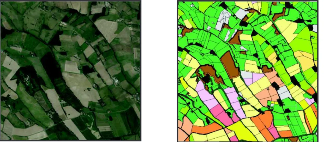
Spatial data is needed to initialize our agricultural landscape. We digitized all the spatial components of the landscape and assigned a cover information for each of them (Figure 1). Fields were characterized by the main crop grown on each of them between 2011 and 2012. The level of detail required in the characterization of each spatial element depends directly on the needs of the user, but it is essential to obtain a fully digitized landscape. Table 1 shows the different spatial entities taken into account in our example.
2.4.3 Crop rotations
Crop rotations may be implemented through different methods (Schönhart et al., 2011; Sorel et al., 2010). We do not include follow-up crops in our first version of crop rotations model to test a simple one. Nevertheless, they could be easily implemented too. We defined 9 typical crop rotations with an agronomist (Table 2). Each rotation is represented by a code and defined by its total duration and the annual succession of covers.
If complete data on the rotations of each field is available (i.e. which rotation is assigned and in what year of the rotation is the field currently in), the model can directly take them into account from the shapefile when creating the simulated landscape.
Table 1: The spatial entities digitized in our model represented by their code and their color in our virtual representation. (a) Agricultural fields and (b) fixed elements structuring the landscape.
(a) (b)
CODE NAME COLOR
For Forest SEd South edge NEd North edge Bui Building/Road
Wat Water
Per Permanent pasture
Hed Hedge
CODE NAME COLOR
Cer Cereals Cor Corn Leg Legume Rap Rapeseed Sor Sorghum Sun Sunflower Tem Temporary pasture
Fal Fallow Oth Other crop
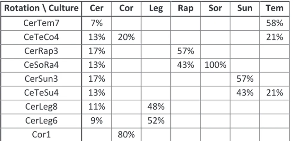
In many cases, this type of information is not available. The model is then able to assign rotations itself. This method relies on the hypothesis that none of the rotations is favored over another one. In order to assign a rotation to each field, the model calculates the probabilities of attribution of each rotation depending on the current cover of the field defined in the previous step. We use the Least Common Multiple of the duration of all rotations to obtain a table where each rotation is repeated a whole number of times and with this same total duration (for more details on how rotations are assigned, see Appendix A). The probability of attribution of each rotation for a particular cover (Table 3) is then calculated using the following formula (1):
!!!!!!!!!!!!!!!!!!!!!!!!!!!!!!!!!!!!!!!!!!!!!!!!!!!!!!!!!!!!!!!!!!!!!!!!"
#=
$%$&'& (1)
Table 2: List of the selected rotations represented by a code and defined by their duration and the succession of covers.
CODE DURATION CULT1 CULT2 CULT3 CULT4 CULT5 CULT6 CULT7 CULT8
CerTem7 7 years Cer Cer Tem Tem Tem Tem Tem CeTeCo4 4 years Cer Cer Tem Cor CerRap3 3 years Cer Cer Rap CeSoRa4 4 years Cer Cer Sor Rap CerSun3 3 years Cer Cer Sun CeTeSu4 4 years Cer Tem Cer Sun CerLeg8 8 years Cer Cer Cer Leg Leg Leg Leg Leg CerLeg6 6 years Cer Cer Leg Leg Leg Leg Cor1 1 year Cor
Cer: cereals: Cor: corn; Leg: Legume; Rap: rapeseed; Sor: sorghum; Tem: temporary pasture.
Where Px is the attribution probability of rotation x for a particular cover, Nx the number of times the cover
appears in rotation x on the total duration and Ntot the number of times the cover appears in all rotation on the
total duration. The model then assigns a rotation to each field according to the cover and the attribution probabilities. Once a year, the cover of the year for each field will be assigned according to the rotation applied to this particular field.
Table 3: Matrix of the attribution probabilities of each rotation depending on the initial cover
Rotation \ Culture
Cer
Cor
Leg
Rap
Sor
Sun
Tem
CerTem7
7%
58%
CeTeCo4
13%
20%
21%
CerRap3
17%
57%
CeSoRa4
13%
43% 100%
CerSun3
17%
57%
CeTeSu4
13%
43%
21%
CerLeg8
11%
48%
CerLeg6
9%
52%
Cor1
80%
Cer: cereals: Cor: corn; Leg: Legume; Rap: rapeseed; Sor: sorghum; Tem: temporary pasture.
2.4.4 Crop phenology
As stated before, crop phenology is an important factor when modeling population dynamics of animals that have their life cycle directly linked to crop availability. In our example, we focus on aphid populations associated to cereals, sorghum and corn. Crop phenology is updated at a daily time step. To determine when the crop becomes available, the user needs to input a date on which farmers can start sowing the crop and
H.Thierry et al. / Managing agricultural landscapes favouring ecosystem services …
the number of degree-days needed for this crop to become available (phenological state) for the studied population and harvested (Table 4). From this date, each field that will grow the crop on this year is assigned a delay value from 1 to 15 days. This delay covers the constraints the farmer can face determining the date he will actually be able to sow his field (machine availability, personal schedule…). Once the delay value reached, the model checks if it is a rainy day. If so, the sowing is delayed to the next day and so on until the weather conditions allow sowing. Once the field is sowed, the model calculates the number of degree-days cumulated each day. Once the value needed for the crop to become available is reached, the model updates the cover of the field. The same method is used for harvesting. Once the crop is harvested, the crop to be grown for the following year is automatically updated according to the assigned rotation of the field. Crops that are not of interest for aphid populations are based on a date to date method for sowing and harvesting.
Table 4: Date on which the sowing of the crop starts and number of degree-days needed for it to become available
Crop Date on which the sowing starts Degree-days needed to become available for aphids
Degree-days needed to be harvested Cereals November 1st 150 1600 Corn April 1st 80 1800 Sorghum April 1st 80 1800 2.4.5 Climatic parameters
Weather conditions are used for biological purposes. Temperature and wind conditions are automatically updated at each time step according to data collected from a weather station in our landscape. It is possible to easily add this type of data in the form of csv tables.
3 RESULTS AND DISCUSSION
Figure 1 shows the landscape representation provided by the model beside a satellite image of the real landscape. . We are currently gathering data on the distribution of crop covers in the LTER landscape each year in order to compare and validate our simulated landscape with the real one.
Figure 1: Satellite image (2010) and simulated landscape (based on the 2012 land-cover) (see Table 1 for color codes). The simulated landscape is 2km x 2km. The satellite image is an IGN orthophotograph
(BDortho®) with a spatial resolution of 0.5m.
The most relevant result is the spatial structure of our landscape over the course of the year. Figure 2 shows how the crop covers evolve, illustrating heterogeneity of agricultural landscapes in terms of crop availability. Insect populations that rely on specific crops to fulfill their life cycle can face each year a totally different scenario in terms of location, date of availability and amount of resources in the landscape
Figure 2: Evolution over time of a part of the virtual landscape (from left to right:1st day, 100th day and 150th day of simulation).
Another interest of using the GAMA platform is the possibility to have a 3D visualization of the landscape. Although we do not currently use these outputs for simulation, it can play an important role both to analyze movement of individuals or populations in space and to help understanding of the model and communication with users. In fact, it allows actors to easily picture the different spatial components of the landscape. It also can be an important support when combining population dynamics with wind-induced movements for example. Spatial elements such as hedges or woods can create wind breaking effects and influence wind conditions in the landscape (Bowden and Dean, 1977; Epila, 1988; Lewis, 1969). Crop heights can also be specified according to their growth since it can also have an impact on insect populations. For example, different species of bees tend to forage on different heights of crops (Hoehn et al., 2008; Sjödin et al., 2008). The validation of the model shall include the comparison between the evolution of crop covers (total area of each crop) throughout the years with data collected on the field.
As this model is intended to be linked to population dynamics, the studied species will evolve directly on the virtual landscape, being influenced by the patches and their covers. The landscape generated illustrates the heterogeneity of agricultural landscapes. The period during which this crop is available depends highly on human factors (simulated through the factors that can influence the date of sowing) and weather conditions (rain, temperature). Thus, changes in the periods of availability of crops as well as crop mosaic throughout the landscape can highly impact population dynamics through facilitation or limitation of dispersal and colonization processes. Studying these changes with our model could lead to a better understanding of how both elements interact. Of course, crops are not the only element that can influence population dynamics. Hedges and forests can influence hoverfly populations too. We are therefore currently developing our model in order to be able to modify the quantity and location of these structural elements in the landscape to test their influence on hoverfly populations and thus on predator-prey interactions.
Taking account these elements together could lead to better understanding how agricultural landscapes influence population dynamics and give us hints on how to improve related ecosystemic services by favoring particular populations through landscape managing.
CODE NAME COLOR
Cer Cereals Cor Corn Leg Legume Rap Rapeseed Sor Sorghum Sun Sunflower Tem Temporary pasture
Fal Fallow Oth Other crop
CODE NAME COLOR
For Forest SEd South edge NEd North edge Bui Building/Road
Wat Water
Per Permanent pasture
H.Thierry et al. / Managing agricultural landscapes favouring ecosystem services …
4 CONCLUSION
With our model we manage to simulate a virtual agricultural landscape with crop rotation and crop phenology dynamics. It is applicable to any agricultural landscape by simply changing the input data. The time step, weather conditions, rotations and covers are defined by the user according to his needs. Adding population dynamics requires knowledge of the multi-agent platform and of agent-based modeling.
The ecological model based on aphid and hoverfly populations will be used as a applied example on how population dynamics can be implemented.
Spatial and temporal scales have to be chosen according to the ecological question behind the use of the model. One of the main interests of the model is to take into account crop phenology which plays an important role when linking landscape effects to population dynamics that directly depend on crops as food or shelter. Developing our model directly in an IBM platform allows to easily connect to individual based simulations with the generated landscape.
The model is reliable but can still be highly improved in terms of integration of agricultural practices. Even if typical crop rotations can be identified, farmers and advisers often face many factors that induce a lot of variability in their choices. Modelling the effects of weather, soil or economic conditions could highly upgrade the realism of our agricultural landscape by improving crop choices through time. Data on the farming practices (pesticides, ploughing…) could also be added for each field. Further research will be dedicated to testing the interactions between our virtually generated landscapes and insect population dynamics.
REFERENCES
Altieri, M., Nicholls, C., 2004. Biodiversity and pest management in agroecosystems. CRC Press.
Arrignon, F., Deconchat, M., Sarthou, J.-P., Balent, G., Monteil, C., 2007. Modelling the overwintering strategy of a beneficial insect in a heterogeneous landscape using a multi-agent system. Ecol. Model. 205, 423–436. Aubertot, J., Barbier, J., Carpentier, A., Gril, J., Guichard, L., Lucas, P., Savary, S., Sav ini, I., Voltz, M., 2005.
Pesticides, agriculture et environnement : Réduire l’utilisation des pesticides et en limiter les impacts environnementaux. Synthèse de rapport d ’expertise.
Bowden, J., Dean, G.J.W., 1977. The distribution of flying insects in and near a tall hedgerow. J. Appl. Ecol. 343–354. Epila, J.S.O., 1988. Wind, crop pests and agroforest design. Agric. Syst. 26, 99–110.
Gaucherel, C., Giboire, N., Viaud, V., Houet, T., Baudry, J., Burel, F., 2006. A domain-specific language for patchy landscape modelling: The Brittany agricultural mosaic as a case study. Ecol. Model. 194, 233–243.
Grignard, A., Taillandier, P., Gaudou, B., Vo, D.A., Huynh, N.Q., Drogoul, A., 2013. GAMA 1.6: Advancing the art of complex agent-based modeling and simulation, in: PRIMA 2013: Principles and Practice of Multi-Agent Systems. Springer, pp. 117–131.
Hoehn, P., Tscharntke, T., Tylianakis, J.M., Steffan-Dewenter, I., 2008. Functional group diversity of bee pollinators increases crop yield. Proc. R. Soc. B Biol. Sci. 275, 2283–2291.
Landis, D.A., Wratten, S.D., Gurr, G.M., 2000. Habitat management to conserve natural enemies of arthropod pests in agriculture. Annu. Rev. Entomol. 45, 175–201.
Lewis, T., 1969. The distribution of flying insects near a low hedgerow. J. Appl. Ecol. 443–452.
Médiène, S., Valantin-Morison, M., Sarthou, J.-P., de Tourdonnet, S., Gosme, M., Bertrand, M., Roger-Estrade, J., Aubertot, J.-N., Rusch, A., Motisi, N., 2011. Agroecosystem management and biotic interactions: a review. Agron. Sustain. Dev. 31, 491–514.
Parker, D.C., Manson, S.M., Janssen, M.A., Hoffmann, M.J., Deadman, P., 2003. Multi-Agent Systems for the Simulation of Land-Use and Land-Cover Change: A Review. Ann. Assoc. Am. Geogr. 93, 314–337. doi:10.1111/ 1467-8306.9302004
Parry, H.R., Evans, A.J., 2008. A comparative analysis of parallel processing and super-individual methods for improving the computational performance of a large individual-based model. Ecol. Model. 214, 141–152. doi:10.1016/ j.ecolmodel.2008.02.002
Parry, H.R., Evans, A.J., Morgan, D., 2006. Aphid population response to agricultural landscape change: A spatially explicit, individual-based model. Ecol. Model. 199, 451–463. doi:10.1016/ j.ecolmodel.2006.01.006 Schönhart, M., Schmid, E., Schneider, U.A., 2011. CropRota–A crop rotation model to support integrated land use
assessments. Eur. J. Agron. 34, 263–277.
Sjödin, N.E., Bengtsson, J., Ekbom, B., 2008. The influence of grazing intensity and landscape composition on the diversity and abundance of flower-visiting!insects.!J.!Appl.!Ecol.!45,!763–772.!
Sorel,!L.,!Viaud,!V.,!Durand,!P.,!Walter,!C.,!2010.!Modeling!spatio-temporal!crop!allocation!patterns!by!a!stochastic! decision!tree!method,!considering!agronomic!driving!factors.!Agric.!Syst.!103,!647–655.! Tenhumberg,!B.,!Poehling,!H.-M.,!1995.!Syrphids!as!natural!enemies!of!cereal!aphids!in!Germany:!aspects!of!their! biology!and!efficacy!in!different!years!and!regions.!Agric.!Ecosyst.!Environ.!52,!39–43.! Tscharntke,!T.,!Tylianakis,!J.M.,!Rand,!T.A.,!Didham,!R.K.,!Fahrig,!L.,!Batary,!P.,!Bengtsson,!J.,!Clough,!Y.,!Crist,!T.O.,! Dormann,!C.F.,!2012.!Landscape!moderation!of!biodiversity!patterns!and!processes-eight!hypotheses.! Biol.!Rev.!87,!661–685.!
H.Thierry et al. / Managing agricultural landscapes favouring ecosystem services …
Appendix A. Details on how rotations are assigned to the patches.
First the model is based on a table summarizing the different rotations.
CODE DURATION CULT1 CULT2 CULT3 CULT4 CULT5 CULT6 CULT7 CULT8
CerTem7
7 years
Cer
Cer
Tem
Tem
Tem
Tem
Tem
CeTeCo4
4 years
Cer
Cer
Tem
Cor
CerRap3
3 years
Cer
Cer
Rap
CeSoRa4
4 years
Cer
Cer
Sor
Rap
CerSun3
3 years
Cer
Cer
Sun
CeTeSu4
4 years
Cer
Tem
Cer
Sun
CerLeg8
8 years
Cer
Cer
Cer
Leg
Leg
Leg
Leg
Leg
CerLeg6
6 years
Cer
Cer
Leg
Leg
Leg
Leg
Cor1
1 year
Cor
We then calculate the number of times each cover appears for every rotation.
Cer
Cor
Leg
Rap
Sor
Sun
Tem
TOTAL
2
5
7
2
1
1
4
2
1
3
2
1
1
4
2
1
3
2
1
1
4
3
5
8
2
4
6
1
1
The least common multiple of the rotation durations is then calculated. In our case it is 168. This means we need to repeat each rotation during 168 years to obtain a table where each of them is repeated an entire number of times. With this number, we calculate how many times each cover appears during these 168 years for each rotation.
Cer
Cor
Leg
Rap
Sor
Sun
Tem
TOTAL
48
120
168
84
42
42
168
112
56
168
84
42
42
168
112
56
168
84
42
42
168
63
105
168
56
112
168
168
168
Finally, we calculate the probability of attribution of a rotation for each cover by simply dividing the number of times the cover appears in the specific rotation by the number of times is appears in all rotations combined.