Pépite | Détection automatique de cris dans le métro

Texte intégral

(1)Thèse de Pierre Laffitte, Lille 1, 2017. Doctoral Thesis Lille University of Science and Technology. Automatic Detection of Screams and Shouts in the Metro. Author: Pierre LAFFITTE In fulfillment of the requirements for the degree:. Docteur en Traitement du Signal et de l’Image 13 December 2017. Thesis committee:. Geoffroy PEETERS - Senior Researcher at IRCAM - Reporter Slim ESSID - Professor at TelecomParisTech - Reporter Laurent Daudet - Professor at Paris Diderot University - Examiner Corinne Fredouille - Associate Professor at Université d’Avignon et des Pays du Vaucluse - Examiner. Laurent Girin - Professor at Grenoble-INP - Thesis Director Charles Tatkeu - Professor at IFSTTAR - Thesis Director David Sodoyer - Associate Researcher at IFSTTAR - Thesis Advisor. © 2017 Tous droits réservés.. lilliad.univ-lille.fr.

(2) Thèse de Pierre Laffitte, Lille 1, 2017. 2. © 2017 Tous droits réservés.. lilliad.univ-lille.fr.

(3) Thèse de Pierre Laffitte, Lille 1, 2017. Contents. 1. Introduction. 2. Automatic Sound Classification: General principles and state of the art 2.1 Fundamentals of Pattern Recognition . . . . . . . . . . . . . . . . . . 2.1.1 Learning-Based Classification . . . . . . . . . . . . . . . . . . . 2.1.2 Classification of sequences . . . . . . . . . . . . . . . . . . . . 2.1.3 Multi-label Classification . . . . . . . . . . . . . . . . . . . . . 2.1.4 Generative Models . . . . . . . . . . . . . . . . . . . . . . . . . 2.1.5 Discriminative Models . . . . . . . . . . . . . . . . . . . . . . . 2.1.6 Artificial Neural Networks . . . . . . . . . . . . . . . . . . . . 2.1.7 Sequence modelling with Neural Networks . . . . . . . . . . . 2.1.8 Post-processing for final decision . . . . . . . . . . . . . . . . . 2.1.9 Evaluation Metrics . . . . . . . . . . . . . . . . . . . . . . . . . 2.2 Related works . . . . . . . . . . . . . . . . . . . . . . . . . . . . . . . . 2.2.1 Environmental Sound Recognition . . . . . . . . . . . . . . . . 2.2.2 Applications . . . . . . . . . . . . . . . . . . . . . . . . . . . . . 2.2.3 Polyphonic Sound Event Detection . . . . . . . . . . . . . . . . 2.3 Conclusion . . . . . . . . . . . . . . . . . . . . . . . . . . . . . . . . . .. 3. 4. 1. Theory of Neural Networks 3.1 From linear models to Deep Neural Networks . . . . . . . . . . . 3.1.1 Linear Models for Classification . . . . . . . . . . . . . . . 3.1.2 The Multi-Layer Perceptron and (Deep) Neural Networks 3.1.3 Generative pre-training . . . . . . . . . . . . . . . . . . . . 3.2 Convolutional Neural Networks . . . . . . . . . . . . . . . . . . . 3.3 Recurrent Neural Networks . . . . . . . . . . . . . . . . . . . . . . 3.4 Conclusion . . . . . . . . . . . . . . . . . . . . . . . . . . . . . . . . Data 4.1 Data recording . . . . . . . . . . . . . . . . . . . 4.2 Database labeling . . . . . . . . . . . . . . . . . 4.3 A short data analysis . . . . . . . . . . . . . . . 4.3.1 Examples of scream/shout realisations. . . . .. . . . .. . . . .. . . . .. . . . .. . . . .. . . . .. . . . .. . . . .. . . . .. . . . .. . . . . . . . . . . .. . . . . . . . . . . .. . . . . . . . . . . . . . . . . . . . . . . . . . .. . . . . . . . . . . . . . . . . . . . . . . . . . .. . . . . . . . . . . . . . . . . . . . . . . . . . .. . . . . . . . . . . . . . . . . . . . . . . . . . .. . . . . . . . . . . . . . . . . . . . . . . . . . .. . . . . . . . . . . . . . . . . . . . . . . . . . .. . . . . . . . . . . . . . . . . . . . . . . . . . .. . . . . . . . . . . . . . . . . . . . . . . . . . .. . . . . . . . . . . . . . . .. 5 6 6 8 13 14 17 17 20 21 22 24 24 25 26 27. . . . . . . .. 29 30 30 35 37 40 42 47. . . . .. 49 50 51 52 52. i © 2017 Tous droits réservés.. lilliad.univ-lille.fr.

(4) Thèse de Pierre Laffitte, Lille 1, 2017. 4.4 5. 6. 7. 4.3.2 Acoustic properties of the subway environment . . . . . . . . . . . . . . . . . 4.3.3 Scream/shout/speech and environment noise together . . . . . . . . . . . . . Conclusion . . . . . . . . . . . . . . . . . . . . . . . . . . . . . . . . . . . . . . . . . . .. Classification of 3 classes for the detection of shouts and screams 5.1 Class Definition . . . . . . . . . . . . . . . . . . . . . . . . . . . 5.2 Experimental settings . . . . . . . . . . . . . . . . . . . . . . . . 5.2.1 Data . . . . . . . . . . . . . . . . . . . . . . . . . . . . . 5.2.2 Metrics . . . . . . . . . . . . . . . . . . . . . . . . . . . . 5.2.3 Features . . . . . . . . . . . . . . . . . . . . . . . . . . . 5.2.4 NN settings . . . . . . . . . . . . . . . . . . . . . . . . . 5.2.5 CNN . . . . . . . . . . . . . . . . . . . . . . . . . . . . . 5.2.6 RNN . . . . . . . . . . . . . . . . . . . . . . . . . . . . . 5.2.7 Post-processing . . . . . . . . . . . . . . . . . . . . . . . 5.2.8 Streaming vs pre-segmented . . . . . . . . . . . . . . . 5.2.9 Training algorithm . . . . . . . . . . . . . . . . . . . . . 5.3 Results . . . . . . . . . . . . . . . . . . . . . . . . . . . . . . . . 5.3.1 Feature testing . . . . . . . . . . . . . . . . . . . . . . . 5.3.2 NN . . . . . . . . . . . . . . . . . . . . . . . . . . . . . . 5.3.3 CNN . . . . . . . . . . . . . . . . . . . . . . . . . . . . . 5.3.4 RNN . . . . . . . . . . . . . . . . . . . . . . . . . . . . . 5.3.5 Streaming vs pre-Segmented . . . . . . . . . . . . . . . 5.4 Conclusion and discussion . . . . . . . . . . . . . . . . . . . . .. . . . . . . . . . . . . . . . . . .. . . . . . . . . . . . . . . . . . .. . . . . . . . . . . . . . . . . . .. . . . . . . . . . . . . . . . . . .. . . . . . . . . . . . . . . . . . .. . . . . . . . . . . . . . . . . . .. . . . . . . . . . . . . . . . . . .. . . . . . . . . . . . . . . . . . .. . . . . . . . . . . . . . . . . . .. . . . . . . . . . . . . . . . . . .. . . . . . . . . . . . . . . . . . .. . . . . . . . . . . . . . . . . . .. 55 57 60. . . . . . . . . . . . . . . . . . .. 61 62 63 63 64 64 64 65 66 66 66 67 68 69 70 75 78 79 80. Integrating contextual information from the acoustic environment: the 15-class task 6.1 Definition of environment/vehicle sound classes . . . . . . . . . . . . . . . . . . . 6.2 Definition of the composite classes . . . . . . . . . . . . . . . . . . . . . . . . . . . 6.3 Experimental settings . . . . . . . . . . . . . . . . . . . . . . . . . . . . . . . . . . . 6.3.1 Data and features . . . . . . . . . . . . . . . . . . . . . . . . . . . . . . . . . 6.3.2 Networks settings . . . . . . . . . . . . . . . . . . . . . . . . . . . . . . . . 6.3.3 Training/testing settings . . . . . . . . . . . . . . . . . . . . . . . . . . . . . 6.3.4 Raw and marginalized confusion matrices . . . . . . . . . . . . . . . . . . 6.4 Results . . . . . . . . . . . . . . . . . . . . . . . . . . . . . . . . . . . . . . . . . . . 6.4.1 Classification of compound classes . . . . . . . . . . . . . . . . . . . . . . . 6.4.2 Marginalizing . . . . . . . . . . . . . . . . . . . . . . . . . . . . . . . . . . . 6.4.3 Environment Classification . . . . . . . . . . . . . . . . . . . . . . . . . . . 6.5 Discussion . . . . . . . . . . . . . . . . . . . . . . . . . . . . . . . . . . . . . . . . .. . . . . . . . . . . . .. . . . . . . . . . . . .. 83 84 85 86 86 86 86 87 88 88 92 94 97. Classification of voice and environment events in a multi-label setting 7.1 Multiple audio sources viewpoint . . . . . . . . . . . . . . . . . . . . 7.2 Multi-label network training . . . . . . . . . . . . . . . . . . . . . . 7.2.1 Notes on multi-label evaluation . . . . . . . . . . . . . . . . 7.3 Class definition in multi-label context . . . . . . . . . . . . . . . . . 7.3.1 Constraining the output . . . . . . . . . . . . . . . . . . . . . 7.4 Experiment Procedure . . . . . . . . . . . . . . . . . . . . . . . . . . 7.4.1 Data and Features . . . . . . . . . . . . . . . . . . . . . . . .. . . . . . . .. . . . . . . .. 99 100 101 101 102 104 104 104. . . . . . . .. . . . . . . .. . . . . . . .. . . . . . . .. . . . . . . .. . . . . . . .. . . . . . . .. . . . . . . .. ii © 2017 Tous droits réservés.. lilliad.univ-lille.fr.

(5) Thèse de Pierre Laffitte, Lille 1, 2017. 7.5 7.6 8. 7.4.2 ANN settings . . . . . . . 7.4.3 Training/testing settings . Results . . . . . . . . . . . . . . . Conclusion and Discussion . . .. . . . .. . . . .. . . . .. . . . .. . . . .. . . . .. . . . .. . . . .. . . . .. . . . .. . . . .. . . . .. . . . .. . . . .. . . . .. . . . .. . . . .. . . . .. . . . .. . . . .. . . . .. . . . .. . . . .. . . . .. . . . .. . . . .. . . . .. . . . .. . . . .. . . . .. 105 105 106 110. Conclusion 111 8.0.1 Perspective . . . . . . . . . . . . . . . . . . . . . . . . . . . . . . . . . . . . . . 116. Bibliography. 128. iii © 2017 Tous droits réservés.. lilliad.univ-lille.fr.

(6) Thèse de Pierre Laffitte, Lille 1, 2017. iv © 2017 Tous droits réservés.. lilliad.univ-lille.fr.

(7) Thèse de Pierre Laffitte, Lille 1, 2017. Chapter. 1. Introduction. 1 © 2017 Tous droits réservés.. lilliad.univ-lille.fr.

(8) Thèse de Pierre Laffitte, Lille 1, 2017. The works presented in this thesis explore a specific area within the field of intelligent surveillance systems for public places. Such systems have been of increasing interest in the past decades, owing in part to growing safety concerns, and to the developments of artifical intelligence and pattern recognition. From video surveillance of public places to signal intrusion and circuit anomaly detection, artificial intelligence has been used if not as a replacement at least as an aid for humans, to monitor the environment and detect abnormal situations. Generally, automatic surveillance systems use the signal acquired from one or more sensors to gather information about the environment in order to automatically make decisions. Video sensors are the most common tools to date, but are not without their faults. The obstruction of the field of vision, potential changes in lighting conditions, are two examples of the limitations of such systems. As a complement, audio offers robustness to those conditions as it inherently does not suffer from the same issues. Some studies have already explored the combination of audio data with data from other sensors, such as video data, and some have started exploring the benefits which could be drawn from the use of audio signals in the framework of surveillance, in different fields of applications such as home intrusion or security in public places. The implications of the type of environment considered are important; the energy level and the variability of the surrounding acoustic environment can be starkly different. This study is set in the context of public transportation, and focuses on an embedded approach, which entails a very particular type of acoustic background which we will present in details later. The objective is to build a system which can automatically detect violent situations in a public transportation system (metro, tramway, etc..), relying on the analysis of the acoustic environment to detect screams and shouts when they occur. To this end we will investigate the use of AI techniques for the analysis of audio signals, within the scope of Neural Networks which will be trained to detect violent situations through the analysis of the audio environment. AI has been used in many ways to analyze audio signals for decades, as the promincence of smartphones can attest; virually all smartphones nowadays are equipped with a voice recognition tool based on AI. Additionally the music industry also shows signs of a growing interest in AI, as its ability to automatically extract and gather information about the music opens up a vast scope of perspective to music providers, the most common applications being music recommender systems, automatic playlist generation, and music identification and recognition [17]. To set the stage, we will outline the basic principles of pattern recognition and how it can be used in the context of audio event detection in Chapter 2. We will break down the problem and see how it can be defined from a classification perspective. The characteristics of audio signals and their representation in the context of classification will be presented and analyzed, as well as the existing methods which can be considered for the task, and their theoretical background. In Chapter 3 we will present the mathematical framework underlying Neural Networks, which will be the basis of the classifiers used to perform our task. We will expound the basis of Linear Models and derive their probabilistic implications, leading to the presentation of the Logistic Regression unit which is the building block of Neural Networks. We then show how the latter use this building block to achieve more complex architectures. Details of different such architectures will be provided (NN, CNN, RNN), outlining their use in audio pattern recognition. Chapter 4 provides a detailed description of the database, collected in a real environment, with realistic simulations of our target application. The realistic conditions will be detailed and their impact on the audio environment will be analyzed. We will show how the resulting database is challenging in its diversity and noisiness, with numerous concurrent sound sources and high energy. A detailed description of the various elements composing it will be provided, in which we 2 © 2017 Tous droits réservés.. lilliad.univ-lille.fr.

(9) Thèse de Pierre Laffitte, Lille 1, 2017. describe the different forms of occurrences of our main target events, screams and shouts, as well as other vocal events, and their relation to the acoustic background environment. In Chapter 5 we consider the problem as a 3-class task, where the classifier has to predict a voice-related class out of the following set: {’shout’, ’speech’, ’background’ }. For this task we will conduct preliminary tests to identify the best feature representation, and the best network configuration for each of the 3 ANN architectures presented in Chapter 3 (NN, CNN, RNN). For each experiment we provide a detailed description of the settings used, before giving the results and drawing conclusions on them. Based on these conclusions we turn to a different approach in Chapter 6, with a view to overcome the difficulties identified in Chapter 5 by taking into account the acoustic background environment explicitely through the addition of different classes. We consider a second labelling scheme which describes the acoustic background environment, and use the classes from that environment to create compound classes with the set of classes used in the previous chapter. We end up with 15 classes, carrying each a description of both voice-related content and environment-related information, on which we perform a 15-class classification. In a last attempt to account for the agressive acoustic background environment we adopt a multi-label paradigm in Chapter 7, where all input data are described with two different labels which the network needs to predict. In this paradigm the classifier learns in a joint fashion both voice-related classes and environment-related information, using its modelling power to predict both at the same time. Finally Chapter 8 will summarize the main aspects viewed in this thesis. We will recall the results obtained with the proposed methods, and draw conclusions as to the relevance of those methods to the task, as well as the lessons we can derive from it. In line with these conclusion we will suggest some ideas for future works and lay out some perspectives.. 3 © 2017 Tous droits réservés.. lilliad.univ-lille.fr.

(10) Thèse de Pierre Laffitte, Lille 1, 2017. 4 © 2017 Tous droits réservés.. lilliad.univ-lille.fr.

(11) Thèse de Pierre Laffitte, Lille 1, 2017. Chapter. 2. Automatic Sound Classification: General principles and state of the art. 5 © 2017 Tous droits réservés.. lilliad.univ-lille.fr.

(12) Thèse de Pierre Laffitte, Lille 1, 2017. 2.1 Fundamentals of Pattern Recognition As stated in the introduction, this work deals with automatic detection of screams and shouts in the subway environment. In this chapter, we present the foundations to address this kind of problem. We start from the general principles of the pattern recognition problem and methodology to address it, and along the way, we progressively introduce the specific case of sound detection and recognition. In the second part of the chapter we complement the start of the art by presenting a series of existing works and applications in related domains.. 2.1. Fundamentals of Pattern Recognition. The automatic detection of specific sounds implies the recognition of audio patterns. This naturally leads to Pattern Recognition, a branch of Machine Learning rooted in Engineering, whose objective is to provide a mathematical solution to the recognition of recurring patterns embedded in raw data. In the following, we outline the general paradigm of Pattern Recognition and its main areas, before delving into its application to audio signal. The broad objective of Pattern Recognition boils down to the assignment of a prediction to an observed input. This prediction can be a pre-defined label which can represent classes, in which case the task is called Classification, or any continuous real value, in which case the task is called Regression. In our case, since we know precisely what we want our system to detect, we can describe it with a pre-defined label. Therefore we will focus solely on Classification here. In practice, making a prediction about some given data requires to take into account the context around the data, which is why we may distinguish the inference stage where the model outputs a mathematical result based on its theoretical setting and on the data, and a “final decision” stage where this result is tempered by a cost before the final decision is made. This cost parameter represents the burden of making a particular decision if it were wrong, in terms of applicative results. A self explanatory example often given is that of a cancer diagnosis: falsly diagnosing a patient with cancer leads to no more than an undully fear, whereas not detecting a cancer in a sick patient has much more serious consequences. The cost of the second mistake should clearly outweigh that of the first one, because it is a much less acceptable mistake. The present work focuses solely on the inference stage and does not intend to investigate the “final decision” stage.. 2.1.1. Learning-Based Classification. Figuratively, the aim of Classification is to split the data into separate groups and put them in different boxes, where each group is associated with a pattern [30]. All models introduced in the following are data-driven, meaning they learn progressively how to classify data by analyzing data. This process is generally divided in two steps: a training stage and a running stage. A dedicated dataset is used for the training stage, allowing the model to learn the general structure of each group. The knowledge acquired during the training stage is then used in the runing stage, when the classifier is provided with new unseen data, to find the most suitable box. In more concrete terms, the boxes are called classes. When the class labels of the training data are known, the learning process is called supervised. Otherwise, it is called unsupervised. In a classification paradigm (as opposed to regression), after being trained on the training dataset, the system provides an estimate of (or a parametric model of) the posterior probability of each class c ∈ [1, C], where C is the number of classes, given a new input data vector xn : yn = {p(c | xn )}c∈[1,C] ,. (2.1). 6 © 2017 Tous droits réservés.. lilliad.univ-lille.fr.

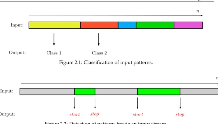
(13) Thèse de Pierre Laffitte, Lille 1, 2017. 2.1 Fundamentals of Pattern Recognition. Figure 2.1: Classification of input patterns.. Figure 2.2: Detection of patterns inside an input stream.. where yn is the output vector consisting of the posterior probability of each class c, and n denotes an index for the input/output sequence, which is often a time index (that will be the case for sound classification). The selected class is the most probable (the one with the highest posterior probability), i.e the class corresponding to the highest value in yn : cˆ = arg max (p(c | xn )) c. = arg max (yn ).. (2.2). c. During the training stage, classification models optimize their parameter values by minimizing a cost function which represents some average classification error over the complete training dataset. This is usually achieved by means of a gradient descent algorithm which sequentially updates the parameters until it reaches a minimum value of the cost function. Classification and Detection. A distinction should be made between Classification and Detection; both rely on the use of a classifier but the difference between the two lies mainly in the way the output of the classifier is dealt with. The goal of Classification is to associate an output class to an input, whereas Detection aims to identify when a certain event occurs within an incoming stream, as exemplified in Figures 2.1 and 2.2. The identification of the moments when the event starts and stops is the main difference between the two. Yet the two processes are closely related. In some cases, Detection is used to perform data segmentation before Classification is applied. In some other cases, Classification is directly used in the process of Detection [112], see Section 2.1.2. Input definition. In order to achieve these objectives, it is necessary to define the input x of these classification/detection systems, especially for temporal signals. Commonly, features are 7 © 2017 Tous droits réservés.. lilliad.univ-lille.fr.

(14) Thèse de Pierre Laffitte, Lille 1, 2017. 2.1 Fundamentals of Pattern Recognition. Figure 2.3: Frame-wise classification of input into output.. extracted from a portion of the signal to be analyzed [92]. Such portions (usually referred to as ’frames’ in audio signal processing) generally have a maximum duration equivalent to the duration of the stationarity of the signal. Thus, the signal is divided in successive frames with same duration, possibly overlapping, where feature vectors are extracted, thereby defining the input x of the classification system.. 2.1.2. Classification of sequences. Frame-wise classification. Frame-wise Classification refers to the case where each input vector is processed individually, i.e. considering each input vector independently of the rest of the input vectors. The classifier produces a corresponding output regardless of past data (and future data in offline / non-causal processing) and past results, thereby dismissing any connection between consecutive inputs. This principle is illustrated in Figure 2.3. Sequence processing. Sequences are a particular type of data in that they consist of ordered frames, which can be uni-dimensional (sequence of scalar values) or multi-dimensional (sequence of vectors; we limit the discussion to the case of fixed-size vectors). They stem from processes evolving in time, with very specific time signatures expressed through the order in which the successive features are arranged. In order to fully ’observe’ a sound it is generally necessary to capture it throughout its entire duration because the essence of a sound often lies in its evolution through time. Indeed, many key characteristics that allow us to distinguish between distinct sounds are time-related (e.g. the attack-decay-sustain-release shape of a note produced by a musical instrument, pitch, envelope, etc..). The temporal dimension therefore often plays a significant role in sound identification (by Humans and machines) and needs to be taken into account in the analysis process. However in this context, frame-wise classification fails to do so. An idea in trying to circumvent this issue is to add temporal context directly into each input vector, in order to force the model to take temporal information into account without drastically changing the structure of the system. This process is called Context Dependency.. 8 © 2017 Tous droits réservés.. lilliad.univ-lille.fr.

(15) Thèse de Pierre Laffitte, Lille 1, 2017. 2.1 Fundamentals of Pattern Recognition Context dependency. The idea is to consider several consecutive frames over a certain period of time, and concatenate the corresponding per-frame vectors to build one unique input vector. This way, the system is fed with information spanning a certain amount of time. We define the following vocabulary and notations: • Context Window: time-span covered by the consecutive frames to form the input, • Context-Dependent Vector (CD vector): ‘new’ input vector resulting from the concatenation of several consecutive single-frame input vectors, • Tw : length of the frame analysis window in seconds, • Th : frame analysis window shift in seconds; If the frame shift is lower than the frame length, there is some overlap between two (or more) consecutive frames, meaning that some part of the information is shared between succesive frame-wise inputs. • Tcd : length of the context window in seconds, • K: length of the context window in number of frames, • D: size (dimension) of each individual single-frame input vector, • S: size of the CD vectors. Tcd , K and Th are linked through the following relation: K=. Tcd − Tw . Th. (2.3). At each time step n, K previous and current (and possibly future) frames are gathered within a context window and concatenated together, as shown in Figure 2.4. The size of this resulting vector is thus K times the size of the single input vector: S = KD.. (2.4). Figure 2.4: Single-frame vectors (top) and Context-Dependent vectors (bottom).. 9 © 2017 Tous droits réservés.. lilliad.univ-lille.fr.

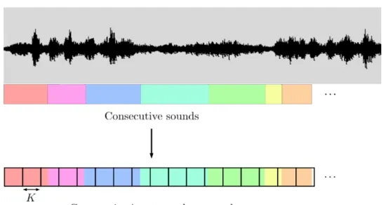
(16) Thèse de Pierre Laffitte, Lille 1, 2017. 2.1 Fundamentals of Pattern Recognition. Figure 2.5: Overlap between successive CD vectors.. Step size and redundancy. There are different ways to build the context-dependent vectors across the dataset, but a step size is generally used to define how the context window should slide over the input frames. A step size lower than the context window size allows to smooth the variations across successive CD vectors, introducing some redundancy at the CD window level, as shown in Figure 2.5 (note that this redundancy adds to the possible redundancy at the frame level, if there is some overlap at the frame level). For example, if the step size is 100 ms and the context window size is 1 s, each super vector spans 1s but is separated by only 100 ms from its predecessor and its successor (measured from a common position in the two vectors, such as the beginning, the middle or the end). This amounts to having 10 super vectors beginning within one second, with an overlap of 90% between them. This means that the super vectors have 90% of similar content, leading to a high amount of redundancy. With a 500 ms step size and a 1 s context window, the overlap goes down to 50%. The redundancy can be avoided by setting a step size equal to the CD window size, but in general, a reasonable amount of redundancy is desirable to smooth the system output sequence and associated decision process (for classification problems). Moreover, overlapping between successive CD windows enables to increase the size of a given dataset without additional data. Note that if the context window shifts by one frame, the classifier makes one decision for each new input frame, just as in frame-wise classification. The difference with frame-wise classification then lies is the fact that the decision is made with more context awareness. If, however, the context window shifts by more than one frame, there are less classification decisions than the original number of frames (before windowing). This is not a problem since the classifier outputs the class that it believes matches the sub-sequence of frames within the context window. In that case, the step size really controls the amount of redundancy across successive context windows, and the data may now be considered as a sequence of context windows, rather than the sequence of original frames. Context dependency and sequence classification for audio signals. Within the framework of audio event detection, the target patterns typically are sequences describing the temporal evolution of the sound spectral content. Frame-wise input vectors are thus vectors of spectral coefficients 10 © 2017 Tous droits réservés.. lilliad.univ-lille.fr.

(17) Thèse de Pierre Laffitte, Lille 1, 2017. 2.1 Fundamentals of Pattern Recognition. Figure 2.6: Left: Three successive sounds are represented by consecutive frames considered as independent one from another. Each color stands for a different sound event. Right: The same sounds are represented with Context-Dependent vectors of K frames. In this example, the size K of the context window is too large with regards to sounds 2 and 3 which are wrongly considered by the classifier as a single event.. representing the short-term distribution of the signal energy as a function of frequency. Typically, the coefficients are modulus square of Discrete Fourier Transform, i.e. an estimate of local power spectral density (PSD), or mel-frequency cepstral coefficients (MFCC), representing the log-scale spectral envelope with a mel-scale frequency axis [111]. Each vector of spectral coefficients is estimated using a time window of size Tw in the range of 10 ms to, say, 60 ms (typically 30 ms) sliding along the signal, generally with some overlap (typically 10 ms) [3, 16, 31]. As stated before, sounds are generally (much) longer than a few tens of ms. Consider the sound of thunder for example; it usually breaks over a few seconds of time, and during the lapse of time before the deep ending sounds occurs, it could be mistaken for a lot of things (cracking beams inside the house, rumbling of a mechanical engine, etc..). This is a perfect example of a succession of different short-term audio patterns (spectro-temporal variation) defining one audio event. Listening to only 30 ms of thunder can be very deceiving if the goal is to identify the source of the sound. To remedy this, Context Dependency, as described earlier, allows the classifier to consider the temporal evolution of sounds over a given duration (defined by the length of the context window). However, the main drawback of this approach is that it defines a fixed context window size of K frames, when different sounds can have (and generally have) different length, and often very different length. The greater the value of K the more chances that two consecutive sounds be captured within the same CD vector. Figure 2.6 illustrates the influence of the number of K frames in the process of creating CD vectors. As a compromise, it is generally better to choose K so that a CD vector is at most as large (on the temporal axis) as the smallest sound event to be recognized, in order to minimize the mixing of successive events in a CD vector. Fixed-sized input machine learning models are relatively easy to implement but they have to face that problem when applied to variable-length temporal signals. Some groundbreaking methods were introduced in order to handle signals of arbitrary length such as Dynamic Time 11 © 2017 Tous droits réservés.. lilliad.univ-lille.fr.

(18) Thèse de Pierre Laffitte, Lille 1, 2017. 2.1 Fundamentals of Pattern Recognition. Figure 2.7: Data formatting following the pre-segmented mode. Different colors indicate different sounds. Hatched regions indicate zero-padding. Note that in this figure (and the following) an elementary compartment of input data represents a CD frame of K input frame-wise vectors, and not one frame-wise vectors as in the previous figures.. Warping [105] and Hidden Markov Models [99]. While DTW can not actually deal with arbitrary length signals, it does allow for variation in length, up to a certain extent. HMMs on the other hand can theoretically deal with infinitely long sequences, but they have their drawbacks. HMMs will be described in Section 2.1.4. Streaming vs pre-segmented. In the literature, automatic sound classification is often performed and evaluated offline with pre-segmented audio patterns (possibly completed with zeros, i.e. a zero-padding pre-process at sound boundaries). In the case of context dependency configuration, this entails that the K frames composing the CD vectors are all from the same sound. However in the present framework of alert signals detection, we have to perform an on-line analysis on an incoming “continuous” audio stream, where the sound patterns that we must detect are thus no longer pre-segmented. In this case, a frame of signal can contain parts of two different sounds and concatenating the K “current” consecutive input frames (for instance the current input frame and the K − 1 past frames) does not necessarily match the onset and offset of the sound patterns: In the neighborhood of class boundaries (when a sound segues into another sound from a different class), a CD vector can contain vectors from the first sound concatenated with vectors from the second sound, which naturally brings some ambiguity in the classification process (test time) and/or the estimation of the models (training time). In that case, in the present work, the label of a CD vector containing segments pertaining to two different classes is chosen to be the class with the highest number of frames within that supervector. This way of formatting and processing a continuous stream data will be referred to as streaming (as opposed to pre-segmented). Figures 2.7 and 2.8 illustrate the difference between the two data formatting processes. In Figure 2.7 the hatched regions represent areas of the input vectors that are padded with zeros in order to match the fixed input size when the sound events do not fit the context window size K exactly. In Figure 2.8 when 12 © 2017 Tous droits réservés.. lilliad.univ-lille.fr.

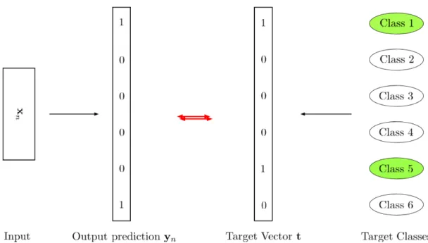
(19) Thèse de Pierre Laffitte, Lille 1, 2017. 2.1 Fundamentals of Pattern Recognition. Figure 2.8: Data formatting following the streaming mode. Different sounds can be mixed up within a same input.. the same situation occurs (where a sound does not fit K) a piece of adjacent sound is used to pad the current input block, instead of zeros. As a result we can see that consecutive sounds can end up mixed together inside an input block, which is naturally expected to make the classification more difficult, as will be verified in our experiments on scream/shout detection in the forecoming chapters.. 2.1.3. Multi-label Classification. So far we have considered the case where each input belongs to one single class, because we relied on the assumption that the classes were mutually exclusive, i.e sounds from different classes could not occur at the same time. However in many real-case scenarios, one may be confronted with the situation where that assumption is not true any more, and sounds from multiple classes can occur at the same time. In that case, the input data needs to be associated with multiple target classes, which is not without consequences on the classification paradigm. This is referred to as multi-label classification as opposed to single-label classification [90, 118]. The classification equation (2.2) for single-label now becomes, for multi-label: ˆ = (yn > γ) c. (2.5). ˆ is the vector containing the estimated classes (potentially multiple in the present multiwhere c label framework) and the right-hand side expression (y > γ) is a boolean expression returning a boolean ’True’ value at all indices where the predicted probability is greater than the threshold γ. In this new paradigm, the classifier has to be able to learn from multi-class training examples, and to output multi-label predictions, as shown in Figure 2.9. The former aspect is addressed by considering the target classes as separate random binary variables (which can thus be on at the same time, indicating that the corresponding events are detected/occurring simultaneously) and then deriving a suitable cost function according to those variables. 13 © 2017 Tous droits réservés.. lilliad.univ-lille.fr.

(20) Thèse de Pierre Laffitte, Lille 1, 2017. 2.1 Fundamentals of Pattern Recognition. Figure 2.9: Illustration of the multi-label classification principle in a 6-class case.. 2.1.4. Generative Models. We have seen how the audio input signal can be represented in the classifier and pre-processed, and we have raised some of the issues related to it. We now turn to the models which will be fed with these inputs, in order to generate a prediction according to Equation (2.2). As defined in this equation, an input feature vector x and a statistical model p(c | x) for each class c are required. For the estimation of p(c | x) two main types of models are defined: Generative models and discriminative models. We rapidly present the generative models in this subsection and we will deal more extensively with the discriminative models in the following of the chapter, since we used the latter in our work. In a classification setting, generative models attempt to model the distribution of the observations x along with the distribution of the target class c, in order to differentiate between classes [10]. Concretely, they use Bayes’ rule to compute the class posterior p(c | x): p(x | c)p(c) p(c | x) = PC b=1 p(x | b)p(b) p(x, c) = PC , b=1 p(x, b). (2.6) (2.7). where we remind that C is the total number of classes. This amounts to modelling the joint distribution of the data and classes p(x, c), which implies that new synthetic data could be created by sampling from this distribution, hence the name Generative. In principle, p(x, c) can be modeled by any probability density model, e.g. the Gaussian distribution. However, it is often the case that not all variables characterizing the set of classes are directly observed through x. These non-observed features call for the concept of “hidden state”. By this paradigm, the complexity of each class is embedded in the expression of one state or multiple states, embodying the different 14 © 2017 Tous droits réservés.. lilliad.univ-lille.fr.

(21) Thèse de Pierre Laffitte, Lille 1, 2017. 2.1 Fundamentals of Pattern Recognition situations (or aspects) which constitute the definition of a class. This entails that only one state can be expressed at a time, meaning that each single datapoint from a class stems from only one state. Generative models considering hidden states include Gaussian Mixture Models (GMMs) [41], Hidden Markov Models (HMMs) [99], Deep Belief Networks (DBNs) [51], etc. In the following we explain the GMM and HMM models, whereas the DBN will be introduced in Section 3.1.3. Gaussian Mixture Models. Mathematically the GMM belongs to the category of Mixture of Experts, which models a target distribution by a weighted sum of parametric components. Here the components are Gaussian and the expression of a GMM is thus: p(x) =. I X. p(h = i)p(x | h = i),. (2.8). i=1. with p(x | h = i) = N (x; µi , Σi ),. (2.9). where I is the total the number of states of the variable h and µi , Σi are respectively the mean vector and the covariance matrix of the Gaussian kernel N (x; µi , Σi ) characterizing state i. πi = p(h = i) P are the weights of the Gaussian kernels in the mixture, with Ii πi = 1. All these parameters can be estimated iteratively during the training process by maximizing the likelihood of the data under the model. A typical algorithm used for such likelihood maximization of GMM parameters is the Expectation-Maximization algorithm (EM) [24]. In a GMM, assuming that one state corresponds to one class, Equation (2.7) amounts to: πc N (x; µc , Σc ) . p(c | x) = PI i=1 πi N (x; µi .Σi ). (2.10). A GMM thus directly provides an estimate of p(c | x) for each class c. This can be easily extended to using several states to model one class. One of the main limitations of GMMs is their inability to deal with sequences, an issue we already mentioned in Section 2.1.2. Nonetheless their association with a temporal model called Hidden Markov Model (HMM) overcomes this issue.. Figure 2.10: Hidden Markov Model with three states.. Hidden Markov Model. An HMM adapts the concept of hidden states to the time dimension by building a sequential model of transitions between states. It thus uses the same concept as GMMs whereby each class is represented by one (or several) hidden state(s), and one observation vector 15 © 2017 Tous droits réservés.. lilliad.univ-lille.fr.

(22) Thèse de Pierre Laffitte, Lille 1, 2017. 2.1 Fundamentals of Pattern Recognition is associated to each state, with the additional property that the states are now part of a Markov chain, i.e. the state hn of the model at (time) step n only depends on the state hn−1 at step n − 1: p(hn | hn−1 , ..., h0 ) = p(hn | hn−1 ).. (2.11). The state transition model is embedded through the transition probabilities ai,j = p(hn = i | hn−1 = j) ruling the possible combinations of states in time, as illustrated in Figure 2.10. If we consider the states sequence: h = h0 , h1 , ..., hn , and the associated observation sequence: X = x0 , x1 , ..., xn , the joint law of (h, X) is : p(h, X) =. N Y. ahn =in ,hn−1 =in−1 p(xn | hn = in ),. (2.12). n. and the distribution of X is the sum of p(h, X) on all the possibilities of h, weighted by p(h). The estimation of p(h0 ), ai,j and of the parameters of conditional observation distributions p(x | h) is performed by the Baum-Welch algorithm [99]. Note that the transitions between states in the presented HMM model are unidirectional, i.e. the process can not go backwards. This type of HMM is called a left-right HMM and is widely used to represent speech phonemes in ASR [99]. Once the model is learned, the problem of estimating a new state sequence given a new observation sequence is solved by the Viterbi Algorithm. Thanks to a smart recursive computation, this algorithm provides the optimal state sequence over the complete (new) observation sequence, i.e. the state sequence with the highest probability, without having to compute the probabilities of all possible state sequences,. For more details on the derivation of the Viterbi algorithm the reader is referred to [99]. Generative models for audio Classification. Applications of Generative models for audio classification include GMMs used to detect gunshots [19, 38], screams [38] and environmental sounds [16]. As mentioned above HMMs [99] and DBNs [97] have been widely used in Automatic Speech Recognition (ASR).. 16 © 2017 Tous droits réservés.. lilliad.univ-lille.fr.

(23) Thèse de Pierre Laffitte, Lille 1, 2017. 2.1 Fundamentals of Pattern Recognition. 2.1.5. Discriminative Models. Discriminative models, on the other hand, attempt to calculate p(c | x) directly. They comprise Logistic Regression, the k Nearest Neighbors algorithm (k-NN), Neural Networks (NN), Support Vector Machines (SVM), etc. Their aim is to find the best separation (according to some metrics) between all classes, resulting in a division of the feature space into one subspace per class. The difference with the generative approach is that here the information about the precise shape of individual distributions of classes is considered poorly relevant. Instead the focus is on the boundaries between classes; the classifier decides which class the data belong to by looking at their location with respect to those boundaries. In short, Discriminative models attempt to separate the classes by finding the shapes of the boundaries between classes, while Generative models attempt to mimic the statistical process that generated the data. The former are commonly considered to be more efficient on classification tasks [86]. Support Vector Machines. Popular Discriminative techniques widely used are the Support Vector Machines (SVMs) and Artificial Neural Networks (ANNs). ANNs will be at the heart of the present thesis work, hence they be will specifically introduced in the next subsection, and their technical description will be made in more details in Chapter 3. Here, we give a few words about SVMs. As a large margin classifier, the SVM assumes that the classes are linearly separable in some feature space, which is obtained by a non-linear transformation Φ of the observation data, resulting in a global a non-linear classifier. In the feature space, a SVM seeks to find the separating hyperplane with maximum distance to the closest points from each class. Such points are defined as support vectors. SVMs make predictions based on kernel functions, defined with respect to the support vectors xsv : k(x, xsv ) = Φ(x)T Φ(xsv ). (2.13) Each new data point is evaluated against the support vectors through the kernel function, and a prediction is made with the following expression: y(x) =. I X. ai ti k(x, xi ) + b,. (2.14). i=1. where ai is the Lagrange multiplier corresponding to support vector i, ti is its corresponding label, and b is a bias term. Similarly to GMMs, SVMs are not tailored for sequences, and need to be associated with a temporal model, such as HMMs (as introduced above) [99] or Dynamic Time Warping (DTW) [69]. The latter is akin to the Viterbi decoder in that it computes the most probable path, but considers the instantaneous state with the highest probability at each time step, instead of the joint probability of the entire path. In the realm of audio applications, SVM (discriminative model) were found to be on par with GMM (generative model) in terms of correct classification scores, but they triggered less false alarms [101].. 2.1.6. Artificial Neural Networks. Artificial Neural Networks (ANNs) are another popular type of Discriminative models. Because they will be the centerpiece of this thesis, Chapter 3 will give a detailed technical description of 17 © 2017 Tous droits réservés.. lilliad.univ-lille.fr.

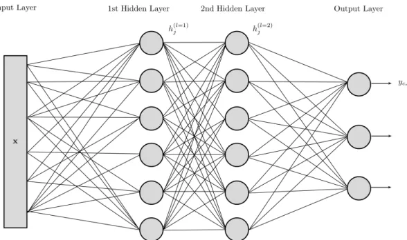
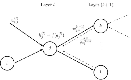
(24) Thèse de Pierre Laffitte, Lille 1, 2017. 2.1 Fundamentals of Pattern Recognition the most popular ANN techniques, and only their general principles will be laid out in the present subsection, in order to give the reader a first broad insight. Artificial Neural Network is a general term that designate a set of discriminative models for pattern recognition, which have been quite popular for some decades now, and used in several fields of applications. All ANNs have in common that they are based on the combination of elementary processing units called ‘neural units’ or ’neurons’ or ’cells’, organized into a network architecture. This network is generally organized in different layers of units. The ouputs of elementary units are connected to the inputs of other units via multiplicative factors called weights. In an ANN, the discriminative information in the input data is thus encoded into the weights of the different layers. Training an ANN on a set of training data consists of setting all the weights values so that the discriminative power of the ANN is maximized on this training set, and hopefully on any test dataset whose distribution is close to the training set distribution, according to the general principle presented in Section 2.1.1. The main advantage of ANNs is that they can learn automatically from the data without requiring any assumption about their distribution, as opposed to parametric classifiers which are generally based on a Bayesian framework, assuming some prior knowledge about the statistical distribution of the data. Most ANNs can be used for both classification (with discrete class-wise outputs) and for regression or generation (with continuous outputs). In the latter case, another strong point is their quality as universal approximators, as explained in [22], giving them the ability to model any non-linear function in compact subsets of R. In the present work, we focus on the use of ANNs as classifiers. As will be seen below, the different types of ANNs mainly differ by the network architecture, by the nature of the neurons, and possibly by some additional processing modules within the network. ANNs can be broadly classified into direct feed-forward Neural Networks, Convolutional Neural Networks, and Recurrent Networks. We introduce now each of these types of ANNs. Direct feed-forward Neural Networks. The structure of a direct feed-forward NNs is illustrated in Figure 2.11. In the following, for simplicity and adequacy with a large part of the literature, this type of ANNs will be simply referred to as Neural Networks (NNs). Such a NN is composed of one or several layers of neurons. Each unit performs a non-linear transformation (called the activation function) on a weighted sum of its inputs, which are the outputs of the previous layer when several layers are used. The first layer, called input layer, is simply the input vector x, and the output layer is composed of output neurons, which compute the posterior probability of each class (one output neuron per class). Intermediate layers between the input and output layers are called hidden layers, and when the number of hidden layers is greater than one, a NN becomes “deep“. The units in hidden layers, noted h, thus operate in chain, building more complicated transformations of the input, with lower layers providing insight of the input data to higher layers, in order to aid the final classification process. The idea is that the resulting non linear functions between inputs and outputs can be arbitrarily complex. Hidden layers. Units in hidden layers are an expression of hidden states, as defined in Section 2.1.4, with the difference that they are no longer exclusive. Indeed, recall from Section 2.1.4 that only one state can be expressed at a time. In NNs on the other hand, the hidden states represented by neurons in hidden layers are elementary units that can be on at the same time. From that perspective they represent hidden factors in the data. These factors are abstractions of the 18 © 2017 Tous droits réservés.. lilliad.univ-lille.fr.

(25) Thèse de Pierre Laffitte, Lille 1, 2017. 2.1 Fundamentals of Pattern Recognition. Figure 2.11: A Neural Network with two hidden layers.. data which are similar to what enables the human brain to understand such data. For instance when hearing the sound made by a dog barking, the brain breaks down the acoustic data into several concepts which interact together, enabling the brain to infer some characteristics of the sound (aggressive, repetitive, loud, etc..). This way it can identify that the sound was made by a dog barking, provided it had previously learned to put a label on this type of sound. The characteristics mentioned here are called high-level abstractions: close to human understanding but far from the original data. Low-level abstractions, on the other hand, might not even be fathomable. The more layers, the more conceptual these abstractions become, enabling the network to discriminate the data more efficiently than if it were working with raw data (which is considered the lowest level of abstraction). In a classification task, the target classes are the highest level of abstraction because they are the last level of abstraction that the model achieves. In light of this explanation on hidden layers, a different perspective can be taken on the operation performed by each individual neuron in the hidden layers (via its activation function) where it can be thought of as an attempt to answer the following question: “Is the input associated with the abstraction or factor associated with the neuron”. In other words, the neurons try to unveil certain characteristics of the input by identifying the features which compose that input. Neurons in higher layers are then able to use those features to pursue their own classification goal on it. History. The first premise of artificial neural networks dates back to 1943 [75], proposing a description of how neurons function in the brain. Several ANN models were then proposed for pattern recognition, using either supervised [100] or unsupervised learning [47]. Deep architectures appeared with [56] and are referred to as Deep Neural Networks (DNN). However it was not until an efficient training algorithm called back-propagation (BP) was popularized by Rumelhart et. al. [102], that deep NN started being used more widely. Yet, DNNs with a lot of layers suffered from an issue known as the vanishing or exploding gradient issue. This major issue of Deep 19 © 2017 Tous droits réservés.. lilliad.univ-lille.fr.

(26) Thèse de Pierre Laffitte, Lille 1, 2017. 2.1 Fundamentals of Pattern Recognition Learning refers to the exponentially plummeting or soaring of the value of error signals when they are propagated back through the network during BP. The more layers, the more prone the network was to suffer from this issue. Deep architectures rose to fame when new training methods were proposed [5, 7, 51], based on graph theory and on the use of a generative model called Restricted Boltzmann Machines (RBM) [33, 52], which subsequently became a tool of choice for pattern recognition tasks. More details about this model will be given in Chapter 3. In the speech community, deep architectures with generative pre-training have been shown to perform better than traditional (HMM-based) methods for automatic speech recognition [98]. Convolutional Neural Networks. Neural Networks have been adapted to image analysis in the form of Convolutional Neural Networks (CNNs), which can analyze 2-dimensional inputs. They were introduced in [34] as a visual pattern recognition technique unaffected by shifts in position. The general principle is that they can process 2-dimensional data by analyzing the input through small windows sliding over both dimensions of the whole input array. Each analysis window is composed of a 2D matrix of weights acting as a 2D-filter, hence the name ’convolutional’. A more indepth decription of the CNNs will be given in Chapter 3.. 2.1.7. Sequence modelling with Neural Networks. A major aspect of the research on NNs in the speech/audio processing community is to study their ability to tackle time sequences, which is essential since, as we have seen in Section 2.1.2, sounds are defined through time, as an evolving process. In this subsection, we present the main approches that have been proposed to efficiently process temporal sequences with NNs. Context-Dependent Neural Networks. One straightforward manner to adapt NNs to analyze temporal sequences is to adopt the context dependency principle described in Section 2.1.2: An input vector to a NN is formed by the concatenation of several single-frame input vectors. In the following, this approach is referred to as Context-Dependent Neural Networks (CD-NNs). NN-HMMs. Another major early attempt to use NNs to process temporal sequences of vectors was made by Bourlard et al. [13] who constructed a hybrid of NNs and HMMs, in which the NNs were used to predict the frame-wise emission probabilities of the HMM states, along the same lines as GMM-HMMs [99]. Recurrent Neural Networks. Recurrent Neural Networks (RNNs) are a special kind of Neural Networks that was devised specifically for sequence modeling. RNNs are built to retain information from past inputs in a dedicated memory. This memory is contained in the hidden units (also often called ’cells’ in the context of RNNs), who are able to retain and accumulate passed information and subsequently use it when necessary to output classification decisions. One basic manner to implement this principle is to set a recurring connection onto the neurons, as illustrated in Figure 2.12: At timestep n a neuron uses as inputs both the current outputs from previous layers (or the input data in case of first layer) and its own past output calculated at time-step n − 1. This way, the information at a given time-step can be carried through several time-steps, enabling temporal integration of the information. 20 © 2017 Tous droits réservés.. lilliad.univ-lille.fr.

(27) Thèse de Pierre Laffitte, Lille 1, 2017. 2.1 Fundamentals of Pattern Recognition hn−1,j. xn. hn,j. Figure 2.12: j th recurrent neuron. Despite their natural ability to learn time structures, RNNs suffered from the vanishing/exploding gradient just like DNNs [8]. As a result, there were only a handful of successful applications of RNNs for speech and language modeling using large RNNs [81]. Long Short Term Memory. To overcome the gradient issues in RNNs, Hochreiter and Schmidhuber [53] came up in 1997 with a variant of RNNs, replacing the classic neurons (made of a unique elementary non-linear function) with (much) more elaborate cells called Long Short Term Memory (LSTM). LSTM cells are capable of encoding temporal information over a long period of time by using a separate ‘container’ variable, the state, where all the information is accumulated. This dual architecture, where memory from previous inputs is retained in a separate pipe, allows the main pipe to access that memory in order to make decisions taking into account information from a long-term past. RNNs using LSTM cells were applied to handwriting recognition [46] and ASR [45]. LSTM networks will be described in more details in Chapter 3.. 2.1.8. Post-processing for final decision. For NNs and RNNs, the estimation of class posterior probabilities is made for every frame-wise input vector xn , hence at every frame index from n = 1 to N . Depending on their implementation, this can also be true for CNNs and context-dependent NNs (if 1-frame shift is applied in the latter case). Depending on the ability of each frame of signal (or CD window, or frame + memory) to represent well the underlying class of sound, a more or less erratic sequence of outputs can be observed, switching from one class to another between two consecutive inputs, which generally makes poor sense since we have seen that sounds generally have a length that is significantly superior to a frame length. To address this issue, post-processing methods are used to filter the sequence of frame-wise outputs and provide a sequence of more consistent final “global” decisions at the sound length level. Two types of filtering methods are considered here: • A smoothing algorithm, • A majority voting algorithm. Note that these methods can been seen as a very simplified version of the NN-HMM approach presented above, where the HMM part is seen as a filtering/smoothing process over the outputs of the NN. 21 © 2017 Tous droits réservés.. lilliad.univ-lille.fr.

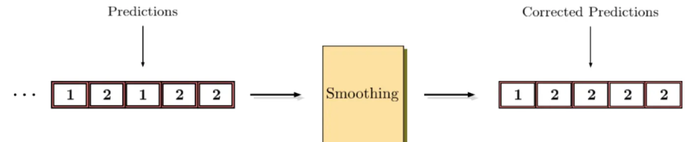
(28) Thèse de Pierre Laffitte, Lille 1, 2017. 2.1 Fundamentals of Pattern Recognition. Figure 2.13: Output corrected by smoothing algorithm.. Smoothing algorithm. The first method prevents a decision at time n from diverging if the two directly adjacent decisions (i.e. at time n − 1 and n + 1) are the same, as shown in Figure 2.13. If the two side predictions are not identical, the algorithm does not do anything. Majority voting algorithm. In the second method, the predictions over a segment of frames of a given length, denoted Tseg , are merged into one unique prediction for the whole segment. To this aim, a majority voting scheme is applied over the segment: The algorithm outputs the class which has the highest number of frame-wise decisions. As a result of this segment detection, the system now outputs one prediction every Tseg seconds (if no overlap exits between consecutive segments). Figure 2.14 gives an example.. 2.1.9. Evaluation Metrics. To finish with the generalities of pattern recognition and its application to audio signals, we present the evaluation metrics that are used to measure the performance of the models as classifiers. To this aim, the following cases are defined, according to [79]: • True Positive (TP): the system detects an event which is present in the input vector. • True negative (TN): the system does not output an event which is not present in the input vector. • False Positive (FP) (aka False Alarm): the system outputs an event which is not present in the input vector. • False Negative (FN) (aka Missed Detection): the system does not output an event which is present in the input vector. Based on those concepts, the number of occurrences of each case on a given test dataset are counted. Then the so-called Precision P and Recall R (or Accuracy) of the system are calculated as: TP P = . (2.15) TP + FP TP R= . (2.16) TP + FN R represents the detection accuracy of the system. It shows how well the system was able to correctly detect the target events in proportion of the number of events to be detected. P is a 22 © 2017 Tous droits réservés.. lilliad.univ-lille.fr.

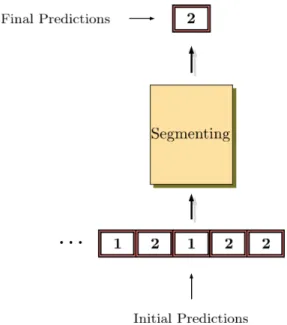
(29) Thèse de Pierre Laffitte, Lille 1, 2017. 2.1 Fundamentals of Pattern Recognition. Figure 2.14: Detection by majority voting over segment of 5 consecutive frame-wise predictions.. measure of the detection quality but in proportion of the number of false alarms. Both values are essential to fully apprehend the system performance. Indeed, if R is high and P is low, the system was able to detect a large amount of the actual targets it was given, but also output a lot of false alarms. Conversely, if R is low and P is high, the system missed a lot of actual targets, but it did not cause a lot of false alarms. Additionally, results are often reported in the form of the geometric mean between Precision and Recall, also called F-score: 2P R F = . (2.17) P +R The results can also be reported in the form of a confusion matrix, where entry ei,j is the percentage of occurrences from class i classified as class j, which makes the diagonal elements of the confusion matrix correspond exactly to the Recall R. While FP and FN give an account of the amount of classification errors without giving any details about which classes were wrongly output, the advantage of the confusion matrix is that it breaks down the number of total errors (i.e. FP+FN) into the wrongly output classes, showing how the misclassified inputs were classified. For more clarity the highest numbers in each line of the confusion matrix are often displayed in bold, representing how the largest proportion of data from class i was classified.. 23 © 2017 Tous droits réservés.. lilliad.univ-lille.fr.

(30) Thèse de Pierre Laffitte, Lille 1, 2017. 2.2 Related works. 2.2. Related works. Our field of application can be seen as part of a more general topic called Environmental Sound Recognition (ESR). ESR refers to the general task of detecting and classifying natural sounds from a continuous audio stream recorded by a microphone or a set of microphones placed in a natural environment. This problem can be further decomposed into Acoustic Scene Classification (ASC) and Sound Event Detection (SED) [3, 116]. In the following we present these two subtopics, then we provide examples of applications.. 2.2.1. Environmental Sound Recognition. Acoustic Scene Classification. ASC deals with the recognition of the type of scene or environment in which the different successive or superimposed recorded sounds occur, e.g. office, restaurant, beach, street, forest, etc. [16, 20, 119]. As illustrated in the former examples, the environments can be indoor or outdoor [11]. The exact nature and time of occurrence of the different sounds composing the scene may not be a relevant target for this kind of problem. Following the principle of supervised training (see Section 2.1.1), for each type of scene/environment, a set of recordings taken from different instances of the considered environment is garnered. The environments instances are usually collected from different locations, in order to display variability. Indeed, the aim is generally to train a model to be able to recognize a given environment regardless of the location of the scene and the location of the microphone within that scene. An example of application is automatic robot orientation, where a robot needs to identify the type of environment in which it evolves [15]. Another type of application is to automatically identify the acoustic characteristics of the scene in order to adapt further specific sound processing, e.g. speech enhancement in noise. Recognition accuracy varies greatly across studies, owing to the variety of the used datasets [15, 29, 70]. In [29] a GMM-HMM is applied on different features (MFCC, energy features, etc.) describing recordings from 24 acoustic scenes (restaurant, marketplace, café, etc.). In [70] MFCCs along with other spectral and energy features are used to describe similar acoustic scenes (15 classes taken from the DCASE challenge [116]). Again, similar features are used in [15] to describe 5 acoustic environments (café, lobby, elevators, outside and hallway). Because both target classes and experimental setups can be very different from one study to another, there is no clear way of evaluating the performances of a model for environment recognition. In 2016 however, a dataset was published to serve as a baseline for environment recognition studies [78]. This followed an effort to bring together the community through the annual DCASE 2016 challenge [116]. Sound Event Detection. As for SED, as explained in Section 2.1.1 the system is expected to detect the different elementary audio events occurring within a continuous audio stream, e.g. car engine whirring, glass shattering, footsteps, etc. Whenever possible, the system should provide their start and end times [118]. Therefore, in addition to the nature of the different classes (general type of acoustic scene vs. specific sounds), the difference between ASC and SED is rooted in the distinction between Classification and Detection outlined in 2.1.1. The CLEAR challenge in 2007 [110] attempted to provide a unified framework for the evaluation of SED methods, in which the metrics account for the system accuracy in determining the temporal boundaries of events. It has since been followed up by the DCASE challenge [116]. Obviously, the task addressed in the present thesis is part of the SED problem. 24 © 2017 Tous droits réservés.. lilliad.univ-lille.fr.

(31) Thèse de Pierre Laffitte, Lille 1, 2017. 2.2 Related works Even if each task has its own specificity, there is quite some overlap in the techniques used for ASC, SED, Music Information Retrieval (MIR) and Automatic Speech Recognition (ASR). In fact, ASR can be seen as a particular case of SED, but due to both huge applicative stakes and the specificity of speech signals, it was historically developed as a topic on its own. Common features can be used in all these tasks, including Mel-Frequency Cepstral Coefficients (MFCC), Mel-Spectrogram, signal statistics, Linear Prediction Coefficients (LPC) [50, 70]. Also, common models were considered, notably Gaussian Mixture Models (GMM), widely used in the early years of ASR, have been applied to scene recognition [3, 116]. Hidden Markov Models, which have been trending in ASR for decades, have been used for the recognition of specific sound events [77].. 2.2.2. Applications. Robotics. As briefly stated above, classifiers for sound recognition have been used in Robotics to help understand the surrounding environment. An audition model is a prerequisite for natural human-robot interaction [57, 121]. Besides embedded ASR models [83, 87], it is useful for the robot to be able to recognize environmental sounds in order to understand the surrounding and scene context so as to better interact with people. Relatively short sounds with very distinctive starting and ending points (such as a door opening, a object dropping, etc..) are considered in [57] while [121] focuses on the detection of abnormal sound events such as glass breaking, gun shooting, screaming, etc.. Speech. Automatic speech recognition is a research topic that has spanned decades. Classifiers are used to recognize sub-word entities, usually defined as phonemes or syllables, in a framework called Acoustic Modeling. Another layer of classification is used to perform what is referred to as the Langage Model. These two models are combined together to perform speech recognition. The most popular technique used in this field for decades has been the Hidden Markov Model (HMM) [2, 60, 73, 99, 124]. In 2015, state-of-the-art unconstrained ASR (no constraint on speaker identity, presence of low-to-notable environmental noise) consists of a combination of very deep DNNs with CNNs and LSTMs trained on huge speech databases (tens of thousands of hours of speech material) [104]. Audio surveillance. This topic of application will be of particular interest to us since it is closely related to the final objective defined for this thesis, namely the detection of screams and shouts. Therefore it appears natural that it should be described in more details than the previous fields of application covered so far. The detection of critical situations is a highly coveted topic in today’s security-related considerations. It is found in numerous distinct research areas such as Computer Vision, Intelligent Surveillance and Audio Event Detection. While most Detection systems are based on visual information [93, 107, 123], the detection of abnormal situations based on audio cues has also been investigated [18, 61], and audio surveillance is now a trending field of application for sound recognition technologies. It requires solid performances from the model as it ideally aims at detecting all targeted sounds while keeping the false alarms rate as low as possible. In [19], two models are built on training data: one for gunshot sounds and another one for ’normal sounds (all other sounds). A decision is taken every 50 ms by selecting the class according to the model with the highest posterior probability across that window. In a second step, three models are built to describe more accurately the gunshot class, which is decomposed in three sub-classes. The classification decision is taken in three stages; the posterior probability of the model for the 25 © 2017 Tous droits réservés.. lilliad.univ-lille.fr.

(32) Thèse de Pierre Laffitte, Lille 1, 2017. 2.2 Related works normal class is compared to each one of the three models for the gunshot classes, and the data is classified as shot if at least one of the gunshot models yields higher posterior probability than the model for the normal class. The features used are MFCC coefficients and spectral statistical moments, along with their first and second derivative, on which Principal Component Analysis is performed. The data is built synthetically by mixing clean gunshot sounds with noise sounds with various Signal to Noise Ratio (SNR). [38] classifies both gunshot and screams. Some novel features are devised, based on the auto-correlation function in order to describe the energy over different time lags and thus differentiate screams, where the energy is rather spread across the duration of the event, and gunshot where the energy is contained in the first time lags. A feature selection process is used to reduce the dimensionality of the data. Two GMMs are used in parallel to discriminate between screams and noise on the one hand, and between gunshot and noise on the other hand. Again, as in [19], the data is artificially built by mixing clean recording of screams and gunshot sounds with noise according to different SNR ratios. [95] aims at detecting shouts in noisy conditions, although the noise is simulated here. MFCC coefficients are used as features and a frame selection process selects the highest energy frame. A GMM is then used to model the selected frames. Three classification rules are used: the first two consider shout versus non-shout but use two different likelihood functions, a two-stage rule separating speech from the rest first, then shout vs non-shout. Security in public places and transportation. [101] presents a system which detects dangerous situations by detecting shouts in an audio stream captured in a real-life environment. A frontend performs segmentation of the stream via the Forward-Backward Divergence algorithm. Each segment is modelled by an auto-regressive models and a transition between two segments is detected when a change in the auto-regressive model is detected. After having discarded irrelevant segments this way, features are extracted from the raw audio in several ways: MFCC, LPC and PLP. A Gaussian Mixture Model (GMM) and a Support Vector Machine (SVM) are then applied to classify the segments. A hierarchical decision tree is built with a binary classifier at each step; the first one aims at discarding short-term noises, the second one, taking as input only the segments not classified as short-term noises by the first one, performs a speech/non-speech classification, feeding the third one with segments classified as speech so that the final decision can be made, classifying into shout/non-shout. The front-end and hierarchical decision tree are deemed useful by performing A/B comparison on training data. Along the same lines, [113] presents a system to detect screams and gunshots, which employs spectral features as well as features based on the autocorrelation function, on top of the classic MFCC coefficients. A feature selection process singles out the features which minimize an objective function. Two GMM classifiers running in parallel discriminate screams and gunshots from noise. As in [101], the input data is recorder in real-life conditions.. 2.2.3. Polyphonic Sound Event Detection. Most SED tasks dealing with real-world applications are confronted with the practical issue of polyphonic audio. Indeed, the acoustic environment generally comprises multiple sources occurring at any given time, which means that sound events can (and often do) overlap. Synthetically created datasets attempt to recreate this polyphony [19, 62] while recordings of live situations are simply naturally subject to it [64]. When single-label classifiers are used, as introduced in Section 2.1.3, they are said to be monophonic in the audio framework, because they can only recognize 26 © 2017 Tous droits réservés.. lilliad.univ-lille.fr.

(33) Thèse de Pierre Laffitte, Lille 1, 2017. 2.3 Conclusion one sound event/source at a time. If those classifiers are applied as is to polyphonic audio data, a monophonic labelling scheme is obtained, inevitably causing some loss of information. Indeed, since only one label can be present at a given time, one would have to disregard other potential events occurring at that same time. Often, such labelling methods are based on the most prominent event [77]. The multi-label paradigm defined in Section 2.1.3 can be used to better process polyphonic audio. As an example, [90] used a multi-label RNN for environmental sound recognition, with sigmoid output activation function and a cross-entropy likelihood function for learning.. 2.3. Conclusion. In this chapter we described the topic of pattern recognition and showed how it is relevant to our problem. More specifically we introduced Classification and explained how it can be used in the context of detection of audio events. The issue of dealing with sequential data was raised and the main difficulties linked to it were exposed, namely the segmentation of data and the variable lengths of patterns. These two aspects must be taken under consideration in our study since as we mentioned audio patterns are sequences with temporal signature. In this context, Context Dependency provides a way to segment the audio data while keeping the temporal information, and pre-segmented and streaming are two approaches providing different ways to go about the problem of the variable length of patterns. The former one ignores the streaming nature of the audio data and focuses on the classification of individual elements, whereas the latter takes it into account. We introduced the multi-label classification paradigm which is useful when several independent audio sources are present in the environment. The mathematical models used to solve all these questions were described, starting with generative models (GMM, HMM) then discriminative ones (SVM, ANN). More details about the way sequences can be handled by ANNs were given, as they constitute the centerpiece of the work presented in the following. Specifically, the RNN, a model designed to provide a way to properly handle sequences, is presented along with its extension with LSTM units. Those units are made to overcome a major training issue of classical RNNs. Two post-processing methods were introduced, which will be used to improve the model’s predictions. Finally, we explained how the models will be tested in the following and how their performance will be tested. The second part of this chapter was dedicated to the presentation of works and studies relying on classification methods, which have been conducted in different fields of application.. 27 © 2017 Tous droits réservés.. lilliad.univ-lille.fr.