Samuelson hypothesis and electricity derivative markets
Edouard Jaeck∗ Delphine Lautier†
April 4, 2014
Abstract
It is common to assert, in the literature on commodity derivative markets, that the be-havior of futures prices is characterized by the "Samuelson Hypothesis" ([27]), i.e. by the presence of a decreasing pattern of volatilities along the prices curve. Despite some debates about statistical measurements, this hypothesis has found a large empirical support. Yet, to the best of our knowledge, one of its empirical implications has never been proposed nor tested: if Samuelson is right, then prices shocks emerging in the physical market should propagate in the direction of the paper market. The first contribution of this paper is to fill this gap. Second contribution: up to now, the validation of the Samuelson hypothesis has never been considered in the case of electricity futures markets. Yet the non storability of this commodity raises interesting questions. Is the Samuelson hypothesis still valid in such a context? What does this new commodity learn us about the role of inventories in the prices’ volatilities? To answer these questions, we examine the prices behavior of the four most important electricity futures markets, worldwide, from 2009 to 2013: two European markets, the German one and the NordPool, the Australian market and the PJM Western Hub in the USA. We use the American crude oil market as a benchmark for a storable commodity ne-gotiated on a mature futures market. We find evidence of a maturity impact for all markets. We finally rely on the notion of indirect storability as a first direction to explain such a result.
JEL Codes: C22, G13, G15, Q41
Key Words: Samuelson hypothesis, Commodity futures, Energy derivative markets This article is based upon work supported by the Chair Finance and Sustainable Develop-ment and the FIME Research Initiative.
∗
DRM-Finance, UMR CNRS 7088, Université Paris-Dauphine, Place du Maréchal de Lattre de Tassigny, 75016 Paris. Email: [email protected].
†
DRM-Finance, UMR CNRS 7088, Université Paris-Dauphine, Place du Maréchal de Lattre de Tassigny, 75016 Paris. Email: [email protected].
1
Introduction and related literature
The most important feature of commodity futures prices dynamics is probably the difference between the behavior of the prices of the first-nearby and deferred contracts. The movements of the former are large and erratic, while the latter are relatively still. This results in a decreasing pattern of volatilities along the prices curve. The same is true for the correlation between the nearest futures price and subsequent prices, which declines with the maturity. This phenomenon is usually called "the Samuelson hypothesis". Intuitively, it happens because a shock affecting the short-term price has an impact on succeeding prices that decreases as maturity increases ([27]). Indeed, as futures contracts reach their expiration date, they react much stronger to information shocks, due to the ultimate convergence of futures prices to spot prices upon maturity. These price disturbances influencing mostly the short-term part of the curve are due to the physical market, and to demand and supply shocks.
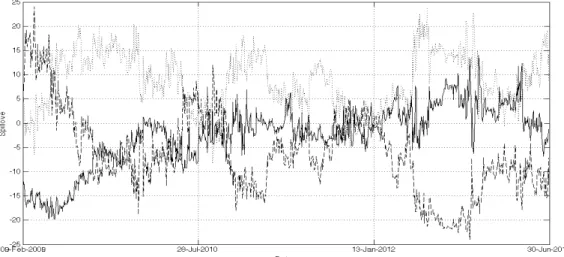
Figure 1 gives an example of such an effect. It represents the prices of electricity on a European futures market (the NordPool) around the Fukushima nuclear disaster of March 2011. The jump recorded in the prices just after the nuclear power plant failure is far more important for short-term than for long-short-term prices. This higher volatility remains obvious in the weeks following it.
The dark line corresponds to short-term futures price (M1); the dashed line is for a most distant maturity (M4). The day of the accident is marked with stars.
Figure 1: Electricity prices around the Fukushima catastrophe, NordPool market (Europe)
Despite some debate about statistical measures, the Samuelson hypothesis has found a large empirical support in the literature, for numerous commodities and for financial assets. See for example among others, Anderson (1985) [3], Milonas (1986) [22], Fama and French (1987)[15], Duong and Kalev (2008) [14], Lautier and Raynaud (2011) [20].
A link between the volatility behavior and the stocks level also appeared quite rapidly. The economic reasoning beyond this link is simple: short-term futures prices might be submitted to contradictory forces. On the one hand, shocks emerging in the physical market of the underlying asset impact them primarily, which results in a higher volatility. On the other hand, a temporary excess of inventories in the market might act as a cushion and decrease the volatility of such
prices1.
In line with this reasoning, Fama and French (1988) [16] test the following proposition: violations of the Samuelson effect might occur at short-term horizon when inventory is high. More precisely they show that for industrial metals, when inventory is high, spot and futures prices have the same variability, whereas in the case of a scarcity, there is a decreasing pattern of volatilities. This proposition is based on the storage theory. It relies on the idea that the marginal conve-nience yield is a non monotonic and decreasing function of the inventory level (see for example Working (1949) [30], Brennan (1958) [6]). Such a phenomenon is confirmed on the basis of an extended analysis by Routledge et al. (2000) [25]. They propose an equilibrium model of the term structure of forward prices for storable commodities which puts emphasis on the non nega-tivity constraint on inventory and takes into account the presence of long-term contracts. They suggest that price volatilities can increase with the maturity of the nearest contracts, because with large inventories, stocks-outs may not be possible in the short-run. A further step was made by including storage costs in the analysis: Deaton and Laroque (1992 [10], 1996 [11]), as well as Chambers and Bailey (1996) [8] indeed showed that the Samuelson effect is a function of the storage cost of the commodity under consideration. More precisely, a high cost of storage leads to relatively little transmission of shocks via inventory across periods. As a result, the futures price’s volatility declines rapidly with the maturity.
Finally, on the theoretical point of view, Bessembinder et al. (1996) [4] propose to establish a relationship between the Samuelson Hypothesis and the storability of the commodity. Focusing on mean reversion in prices, which is the direct consequence of storability, they show that the hypothesis should be observed only for storable commodities.
Such conclusions raise questions about the dynamic behavior of futures prices in electricity futures markets. Up to now, to the best of our knowledge, the validation of the Samuelson hypothesis has never been considered at a large scale for this new commodity (one mention however must be made about Walls (1999) [29], who proposes a study on a sample limited to 14 futures contracts for the PJM). Yet its non-storability raises interesting questions. Is the Samuelson hypothesis still valid in such a context? What does this commodity learn us about the role of inventories in the prices’ volatilities? Recent advances, both on the theoretical and on the empirical side, give a direction to answer such questions. As early as in 2001, Routledge et al. (2001) [26] un-derline that the potential storability of electricity in the form of fuels motivates the exploration of the relationship between electricity and fuel prices. This idea was latter reformulated under the notion of "indirect storability" (for a short review on that point, see for example Huisman and Kilic (2012) [17]). Going further, Aïd et al. (2013) [2] propose to consider electricity as a portfolio of futures contracts on its inputs, and show that this is the case on the French market. In this article, we rely on this concept to explain why the Samuelson Hypothesis is validated on electricity markets. We go further by suggesting that there are some directionality effects, from the inputs to the electricity prices.
Of course, testing the Samuelson effect on electricity markets requires a thoughtful analysis of its empirical implications. Up to now, to the best of our knowledge, two implications have been tested.The first one is the most closely linked to the idea developed by Samuelson himself: if prices shocks arising from the physical market influence the futures contracts all the more that these contracts are close to their expiration date, then volatility must be a decreasing function of
1Remark that consequently, the Samuelson effect should be less pronounced for financial assets than for
com-modities. The latter are characterized by a non negativity constraint on inventories that does not operate strongly in the case of financial assets.
the remaining days before maturity (For this, see for example Milonas (1986) [22], Walls (1999) [29], Bessembinder et al. (1996) [4]). Second implication: if there is a decreasing relationship between the volatility and the time-to-maturity, then the volatility of the one-month contract should be higher than the one of the two-month, which in turn must be higher than that of the three-month, etc. In other words, there should be an ordering in the time series of volatilities across maturities, resulting in a decreasing pattern (See Duong and Kalev (2008) [14]).
According to us, if the Samuelson hypothesis is valid, then a third empirical implication arises and must be tested. This implication can be very briefly and simply stated: if futures markets really function as described by Samuelson and as expected as regards to the risk management function of a derivative market ? If the presence of the paper market allows for hedging against prices shocks affecting the underlying asset, then these shocks should emerge in the physical market. Consequently, they should propagate in the direction of the paper market, with a de-creasing intensity when the contract’s maturity rises. Thus, not only should the volatilities be ordered according to the maturity; there should also be volatility spillovers from the physical market to the paper market. In order to test this assumption, we rely on the method recently developed by Diebold and Yilmaz (2012) [13].
Such a careful and global investigation of the Samuelson Hypothesis on electricity markets is important: after having been considered as a public good during decades, electricity is now regarded as a tradable commodity in most developed countries. Since they were launched twenty years ago, electricity derivative markets exhibit sustained rises in their transaction volumes. Even if these markets are still recent, which raises empirical issues such as the lack of historical data or of long dated contracts, there is now enough information to understand precisely how they function and to compare them with other markets for traditional commodities.
More generally, getting a deeper knowledge of the Samuelson hypothesis is interesting for both financial and industrial agents. At first, traditional hedgers on commodity derivatives markets are industrial companies, or even farmers. They use futures markets to hedge their physical exposure to the underlying asset, and they might want to minimize their hedging cost, using futures contracts with the lowest volatility. Secondly, it is essential for financial engineers to take into account the Samuelson hypothesis when pricing options or other derivatives. Indeed, the volatility is one of the most important parameters in existing pricing procedures (Black Scholes, 1973 [5]). The importance of this effect must be emphasized to practitioners as it is the case for the volatility smile. Finally, the maturity impact also concerns clearing houses when they set margin requirements. Indeed, margin requirements, which are supposed to protect against counter-party credit default risk, are function of the risk of the underlying contract, for which a proxy could be the volatility. Taking into account the existence of a Samuelson effect should induce clearing houses to set higher margin requirements for closest-to-maturity contracts.
In this article, we examine the prices behavior of the four most important electricity futures markets worldwide from 2009 to 2013: the German market, the NordPool, the Australian market and the PJM Western Hub in the USA. We also rely on the American crude oil market as a benchmark for a storable commodity negotiated on futures markets and as an example of a mature contract.
The remainder of this paper is organized as follows. In section 2 we describe the data. Section 3 explains how we test the three empirical implications of the Samuelson hypothesis and displays our results. Section 4 goes deeper into the understanding of the maturity impact by introducing in the analysis, first the transaction volumes and second, the prices of electricity inputs. Section
5 concludes.
2
Data and descriptive statistics
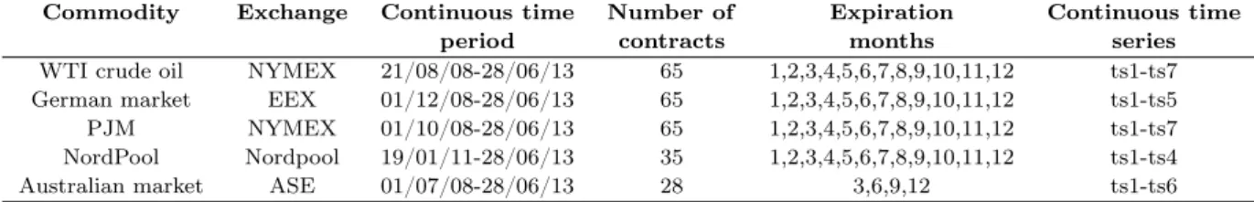
Our database is extracted from Datastream and gathers daily settlement prices of monthly futures contracts2, for four electricity futures markets: the German one, the NordPool (representative of European Nordic countries), the Australian market and the American PJM. These markets are characterized, worldwide, by the most important trading volumes on electricity. In addition, we collected data for the Light sweet crude oil contract (also known as the West Texas Intermediate, hereafter WTI) negotiated on the New York Mercantile Exchange. This market is used as a benchmark in this study, for two reasons: i) on the period under examination, it is the first commodity market as regards to transactions volumes; ii) it is storable. The most important characteristics of these data are summarized in Table 1.
Commodity Exchange Continuous time Number of Expiration Continuous time
period contracts months series
WTI crude oil NYMEX 21/08/08-28/06/13 65 1,2,3,4,5,6,7,8,9,10,11,12 ts1-ts7 German market EEX 01/12/08-28/06/13 65 1,2,3,4,5,6,7,8,9,10,11,12 ts1-ts5 PJM NYMEX 01/10/08-28/06/13 65 1,2,3,4,5,6,7,8,9,10,11,12 ts1-ts7 NordPool Nordpool 19/01/11-28/06/13 35 1,2,3,4,5,6,7,8,9,10,11,12 ts1-ts4
Australian market ASE 01/07/08-28/06/13 28 3,6,9,12 ts1-ts6
This table sums up the features of the data contained in our dataset. Expiration months are numerically repre-sented, that is 1=january, 2=february... For continuous time series, ts1-ts7 means that we created 7 continuous time series. Our sample contains 258 futures contracts, with 193 electricity futures contracts
Table 1: Data features
To give more insight on the markets under consideration, Table 2 exhibits the average vol-umes of contracts traded each year 3 (MW), both maturity by maturity and for all maturities.
Time series WTI Germany PJM NordPool Australia All 77, 252.6 90.7 19.6 121.5 All 23.2 M1 275,248.3 270.8 40.6 332.9 Q1 30.1 M2 136,215.3 120.2 20.1 95.6 Q2 25.4 M3 54,602.3 39.4 17 35.7 Q3 24.8 M4 29,868.9 15.5 18.5 21.8 Q4 25.6 M5 18,781.1 7.4 17.6 Q5 19.6 M6 14,707 17.7 M7 11,345.5
For electricity markets, except for the PJM,1 contract = 1 MW. For the crude oil market, 1 contract represents 1,000 barrels. The first line stands for the mean number of contracts exchanged for all maturities, the others for one maturity. Mi/Qi stand for prices with a i-month/i-quarter maturity.
Table 2: Mean transaction volumes, 2008-2013.
Even if there are important differences between these futures contracts, due to their underly-ing assets (crude oil vs electricity) and also to the contract’s specifications for electricity markets (MW per contract, delivery hours...), a simple glance at the trading volumes makes it clear that electricity futures markets, with mean volumes ranging from 19.6 to 121, stand far away from the crude oil market, characterized by 77,252.6 contracts per year, on average for all maturities.
2
The Australian market, with quarterly expiration dates, is the exception
3
Note also that, as far as the electricity markets are concerned, the NordPool and the German markets have higher volumes. Finally, for all markets, the trading volume is concentrated on the first maturity, and then decreases regularly with the time to expiration. This feature is typical of derivative markets.
As specified in Table 2, our study covers almost five years, between different starting dates in 2008 (August for crude oil, December for the German market, October for the PJM, July for the Australian market) and June 2013. Due to a lack of data for some expiration dates, we also had to reduce the time period for the NordPool: it starts in January 2011.This leaved us with a total of 258 futures contracts. Most of our empirical tests rely on continuous time series of futures prices with constant maturities. Thus while keeping the raw data, we used them to reconstitute daily term structures of futures prices.
Because our dataset contains futures contracts maturing periodically, and because there are, at the same observation date, quotes for contracts with different maturities, we created continuous time series using rolling-over techniques. More precisely, the first time series contains futures prices for the nearest contract, the second futures prices for the second closest-to-maturity con-tract, and so on. The rollover takes place at each expiration date.
Finally, note that the length of the term structure is different for each market: we have maturities up to seven months for the PJM, six for the Australian market, five for the German market and four for the NordPool. As far as crude oil is concerned, even if existing maturities reach several years (up to nine), we retained only the first seven months. Figure 2 represents these continuous time series of futures prices for crude oil and the German electricity market. Charts for other markets are available in the Appendix.
Another comparison between the markets under consideration, focused on the volatility of the futures prices, is given by Table 3. The latter provides, for each market, some descriptive statistics about the volatility of the nearby futures price, for which charts are available in Appendix. In this article, we use the absolute value of the prices returns as a proxy for the volatility (Bessembinder et al. (1996)):
σdaily= | ln(
Ft
Ft−1
)| ∗ 100
where σdaily is the daily volatility, Ft and Ft−1are the settlement prices of a futures contract at different observation dates t and t − 1.
The use of the High-Low volatility measure of Parkinson (1980) [23] and Garman & Klass (1980) [21] was not possible with our data set, due to the lack of data on High and Low prices on certain markets and/or periods.
More precisely, Table 3 exhibits the mean, median, standard-deviation, skewness and kurtosis for the daily volatilities, between 2008 and 2013. We also conducted some statistic tests for the autocorrelation (Ljung-Box test4) and the normality (Jarque-Bera test5) of the series, as well as for the presence of unit-roots (ADF test6).
First remark, the PJM market appears to be the most volatile one, according to both the mean and the median. However, it also has the biggest standard-deviation. The NordPool comes second. Then the crude oil market, followed by the two last electricity markets. This result is rather surprising: the crude oil being the only storable commodity of the sample, one would have
4
H0: The data are independently distributed 5H
0: Normality 6H
(a) Crude oil market: WTI
(b) German electricity market
The solid line is for the nearest maturity, and the dashed line for the most distant maturity
Figure 2: Continuous time series of prices, 2008-2013
WTI Germany PJM NordPool Australia Mean 1,781 1,162 3,852 2,233 1,209 Median 1,204 0,808 2,365 1,671 0,359 Standard-deviation 1,904 1,187 4,872 2,083 2,661 Skewness 2,47 3,54 3,43 2,09 7,15 Kurtosis 11,29 31,12 21,86 9,78 82,32 ADF -17,28* -17,55* -18,96* -11,67* -23,52* LB 1590* 205* 186* 242* 278* Jarque-Bera 4750* 40 679* 20 074* 1623* 342 959* Descriptive statistics of closest-to-maturity time series. ADF is the test statistic of the Augmented Dickey-Fuller test for unit-roots, without lag. LB is the test statistic of the Ljung-Box test for autocorrelation, with 15 lags. Jarque-Bera is the test statistic of the Jarque-Bera test for normality. * means reject of H0 at a 1% level
thought of him as the less volatile.
A second remark is that we can raise some doubts about the normality of our time series of volatilities: all markets have a non-normal skewness, with coefficients ranging between 2.09 and 7.15, which is well above 0. In the same way, with values between 9.78 and 31.12, all markets have a non-normal kurtosis.
Third remark, results are homogeneous as regards to the statistics tests; i) no series contains unit-roots : this allows us to study them without pretreatment; ii) the results of the Ljung-Box test shows the presence of autocorrelations in the time series of volatilities; iii) the Jarque-Bera test confirms that the series do not follow a normal distribution. These results justify the use of non-parametric tests to study the maturity impact on electricity derivatives markets.
3
Does the Samuelson hypothesis hold for electricity markets?
The Samuelson hypothesis has several empirical implications. The first one is the most closely linked to the idea developed by Samuelson himself: if prices shocks arising from the physical mar-ket influence the futures contracts all the more that these contracts are close to their expiration date, then volatility is a decreasing function of the remaining maturity. A second implication is that there should be an ordering in the time series of volatilities across maturity: more precisely, a decreasing pattern should be observed. Finally, shocks propagating from the physical to the paper markets should lead to volatility spillovers. In this section, we successively examine these three implications.
3.1 Is volatility a function of the Time-To-Maturity (TTM)?
As a first test of the maturity impact, we perform a linear regression between all the volatilities and T T M measures available for each market. That is, we regroup in one series all daily volatility measures that we have for one market, and in another series all time-to-maturity measures corresponding, and we run the regression between these two series. We run the regression this way to avoid to run the regression for each one of the 258 futures contracts and have too many estimation results. The linear regression for one market is expressed as follows:
σi = α + βT T Mi+ εi, ∀i ∈ [1, T ∗ N ]
where σi is one volatility, α is a constant, T T Mi is the number of days until expiration7 cor-responding to σi, εt stands for noise, T is the number of observations and N the number of
maturities. As our volatility measure is by definition positive, the same should be true for the coefficient α. Moreover if, according to the Samuelson hypothesis, the volatility increases when the contract reaches maturity, the β should be negative.
Table 4 gives the value of the coefficients, for each market. The results are homogeneous: for each electricity market as well as for the WTI, we obtain positive constants and negative betas. Moreover, all these coefficients (both α and β) are statistically significants at the 1% level. This is consistent with the Samuelson hypothesis. Nevertheless, we can note that our coefficients of determination are low. This comes probably from the fact that, as shown before, our data violate some assumptions8 of the linear regression. We thus consider these results as a first step in the
7
T T Mt decreases when the expiration of the futures contract comes near. 8
WTI Germany PJM NordPool Australia α 1,7653 1,1223 2,7783 2,1637 0,9116 (p-value) (0,00) (0,00) (0,00) (0,00) (0,00) β -0,0023 -0,0037 -0,01697 -0,0118 -0,0014 (p-value) (0,00) (0,00) (0,00) (0,00) (0,00) R2 0,0034 0,0130 0,0998 0,0341 0,0139
Table 4: Coefficients of the linear regression testing wether volatility is a function to the TTM.
validation, that must be confirmed with non-parametric tests.
3.2 Are time series of volatilities ordered?
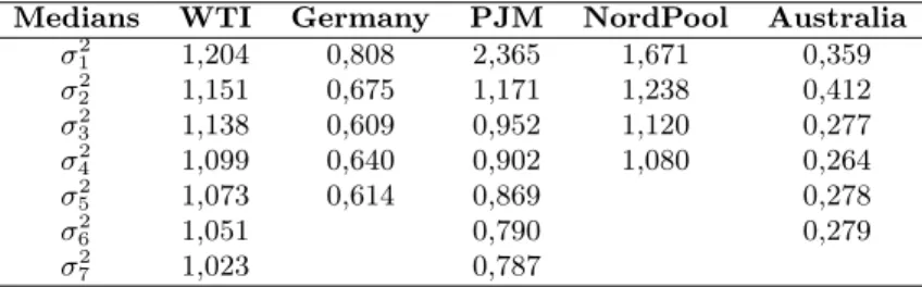
The second implication of the Samuelson hypothesis is that, if there is a decreasing relationship between the volatility and the time-to-maturity, then the volatility of the one-month contract should be higher than the one of the two-month, which in turn must be higher than that of the three-month, etc.
Table 5 reproduces for each market the values of the volatilities - more precisely, their median - according to the maturity. The results stand in line with the Samuelson hypothesis for the crude oil market as well as for the PJM and the Australian market: there is a decreasing term structure of volatilities. For the German market, the volatility of the fourth maturity is higher than expected. For the Australian market, the volatility curve is S-shaped. Remind however that maturities of this market range for 3 to 18 months. They are thus longer.
Medians WTI Germany PJM NordPool Australia σ2 1 1,204 0,808 2,365 1,671 0,359 σ2 2 1,151 0,675 1,171 1,238 0,412 σ23 1,138 0,609 0,952 1,120 0,277 σ24 1,099 0,640 0,902 1,080 0,264 σ25 1,073 0,614 0,869 0,278 σ2 6 1,051 0,790 0,279 σ2 7 1,023 0,787
Medians of time series by maturity. σ2kis the median of tsk.
Table 5: Medians of time series of volatility
The results on the term structure of volatilities are thus contrasted. As a robustness check, we perform, like in Duong & Kalev (2008)[14], a non parametric test. Such a test suits well with our non-normal time series, since it does not assume any particular distribution. More precisely, we use the Jonckheere-Terpstra (JT) test, developed by Jonckheere (1954)[18] and Terpstra (1952)[28], which allows to see if the medians of our time series of volatility are significantly decreasingly ordered by maturity.
Let us describe the null and the alternative hypotheses (respectively H0 and H1) of the JT test as follows:
(
H0 : σk2 = σk−12 = ... = σ21
H1 : σk2 ≤ σk−12 ≤ ... ≤ σ21
where σk2 is the median of the kth time series of volatility. Such a formulation leads to accept the existence of a maturity impact when the null hypothesis of the JT test is rejected.
To perform this test we have to compare the observations of each time series to the obser-vations of another one. In other words, we pair each observation in ts1 with each observation in ts2, in ts3, and so on. For each comparison, we attribute a value of one (zero) if the first member is bigger (smaller) than the second one. A value of 0.5 is recorded in the case of a tie. Finally, we sum up all these values to get the test statistics J. For large sample sizes, the JT test statistics is approximately normally distributed with a zero mean and a variance equals to one.
Z = J − [(N 2−Pk i=1n2i)/4] q [N2(2N + 3) −Pk i=1n2i(2ni+ 3)]/72
where N is the total number of observations and ni the number of observations in tsi.
The results of the JT test are reported in Table 6. It shows that we can reject the null hypothesis at a 1% level for all markets. That is the Samuelson hypothesis holds for the WTI market and for all electricity futures markets studied.
WTI Germany PJM NordPool Australia Z statistics 4,65 7,86 25,18 8,15 4,77
(p-value) (0,00) (0,00) (0,00) (0,00) (0,00) Z-statistics and p-value of the Jonckheere-Terpstra test, which examines the null hypothesis of equals medians, against the alternative hypothesis of ordered medians. Reject H0 implies to accept the Samuelson hypothesis.
Table 6: Jonckheere-Terpstra Test
3.3 Do prices shocks spread from the physical to the paper market?
Another reading of the Samuelson hypothesis should finally, lead to the analysis of volatility spillovers: the prices shocks, measured by the volatility, should spread to the paper market with a decreasing intensity when the contracts’ maturity rises. More precisely, not only should the volatilities be ordered according to the maturity; there should also be volatility spillovers from the physical market in the direction of the paper market (Lautier and Raynaud, 2014). In order to test this third implication, as usually done in finance, we use the first nearby contract as a proxy for the spot price, and we rely on the volatility spillover measure of Diebold and Yilmaz (2012) [13]. We first present this measure. We then expose our results.
3.3.1 Spill over measures: methodology
Diebold and Yilmaz (2012) [13] developed measures of directional volatility spillovers and used them to observe how volatility spills over across markets. In our case, the method is used for different maturities of the same futures contracts.
These measures are extensions of the DY spillover index developed by Diebold and Yilmaz (2009) [12], and improve it in two ways: i) the DY spillover index was only an index of total spillover. This means that it tells us how much volatility spreads across all our markets but does not provide information about the direction of this spillover. On the contrary, the volatility spillover measures developed in 2102 allow to compute measures of directional volatility spillovers, and then to see from which market and to which one the volatility spillover takes place; ii) the DY spillover index was based on a simple vector autoregressive (VAR) framework for which results
can be order-dependent due to the Cholesky factor orthogonalization, whereas the measures of 2012 are based on a generalized vector autoregressive framework in which forecast-error variance decompositions are invariant to the variable ordering.
Authors consider a covariance stationary N-variable VAR(p), xt = Ppi=1φixt−i+ εt, where
ε ∼ (0, Σ) is a vector of independently and identically distributed disturbances. The moving average representation is xt =P∞i=0Aiεt−i, where the N × N coefficient matrices Ai obey the
recursion Ai = φ1Ai−1+ φ2Ai−2+ ... + φpAi−p, with A0 being an N × N identity matrix and with
Ai = 0 for i < 0. They use the moving average coefficients to understand the dynamics of the
system with variance decompositions. The variance decompositions allow to assess the fraction of the H-step-ahead error variance in forecasting xi that is due to shocks to xj, ∀j 6= i, for each
i.
Authors rely on the generalized VAR framework of Koop, Pesaran, and Potter (1996) [19] and Pesaran and Shin (1998) [24] (KPPS) to avoid the use of the Cholesky factorization to have orthogonal innovations, in which the variance decompositions then depend on the ordering of the variables. The KPPS H-steap-ahead forecast error variance decompositions θijg(H), for H = 1, 2, ..., is: θijg(H) = σ −1 jj PH−1 h=0(e0iAhΣej)2 PH−1 h=0(e0iAhΣA0hei)
where Σ is the variance matrix for the error vector ε, σjj is the standard deviation of the error
term for the jth equation, and ei is the selection vector, with one as the ith element and zeros otherwise. Then, each entry of the variance decomposition matrix is normalized by the row sum to compute spillover measures:
˜ θgij(H) = θ g ij(H) PN j=1θ g ij(H)
Finally, using the KPPS variance decomposition, authors developed measures of directional spillovers and net pairwise spillovers.
Directional spillovers give information about the direction of volatility spillovers across mar-kets. Authors measure the directional volatility spillovers received by market i from all other markets j as: Si.g(H) = PN j=1,j6=iθ˜ g ij(H) PN i,j=1θ˜ g ij(H) · 100 = PN j=1,j6=iθ˜ g ij(H) N · 100
In a similar way, they measure the directional volatility spillovers transmitted by market i to all other markets j as:
S.ig(H) = PN j=1,j6=iθ˜ g ji(H) PN i,j=1θ˜ g ji(H) · 100 = PN j=1,j6=iθ˜ g ji(H) N · 100
The net pairwise volatility spillovers gives information about how much market i contributes to the volatility of market j, in net terms:
Sijg(H) = ˜ θjig(H) PN i,k=1θ˜ g ik(H) − ˜ θijg(H) PN j,k=1θ˜ g jk(H) ! · 100 = ˜ θgji(H) − ˜θijg(H) N ! · 100
3.3.2 Empirical results : static analysis
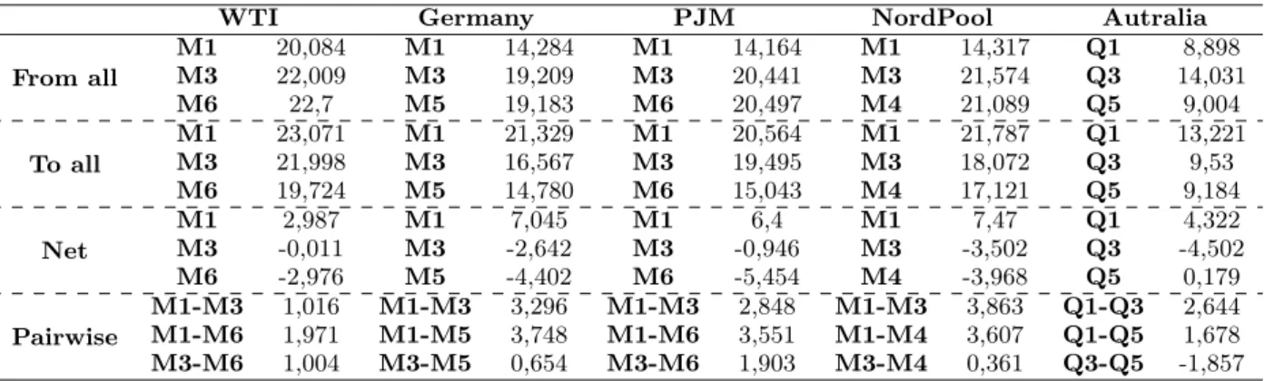
Firstly, we use this framework to measure the volatility spillovers between prices for different maturities for each market on the entire time period. That is, for each market we compute
directional volatility spillovers, and net pairwise spillovers for 3 maturities on our sample period. To do so, as in Diebold and Yilmaz (2012) we use the following parameters: p=4 lags for the VAR, and H=10 for the forecast error variance decompositions.
WTI Germany PJM NordPool Autralia
From all M1 20,084 M1 14,284 M1 14,164 M1 14,317 Q1 8,898 M3 22,009 M3 19,209 M3 20,441 M3 21,574 Q3 14,031 M6 22,7 M5 19,183 M6 20,497 M4 21,089 Q5 9,004 To all M1 23,071 M1 21,329 M1 20,564 M1 21,787 Q1 13,221 M3 21,998 M3 16,567 M3 19,495 M3 18,072 Q3 9,53 M6 19,724 M5 14,780 M6 15,043 M4 17,121 Q5 9,184 Net M1 2,987 M1 7,045 M1 6,4 M1 7,47 Q1 4,322 M3 -0,011 M3 -2,642 M3 -0,946 M3 -3,502 Q3 -4,502 M6 -2,976 M5 -4,402 M6 -5,454 M4 -3,968 Q5 0,179 Pairwise M1-M3 1,016 M1-M3 3,296 M1-M3 2,848 M1-M3 3,863 Q1-Q3 2,644 M1-M6 1,971 M1-M5 3,748 M1-M6 3,551 M1-M4 3,607 Q1-Q5 1,678 M3-M6 1,004 M3-M5 0,654 M3-M6 1,903 M3-M4 0,361 Q3-Q5 -1,857 Net is "To all others - From all others". Pairwise M1-M3 is "From M1 to M3 - To M1 from M3"
Table 7: Volatility spillover across maturities on the entire period
The results, in Table 7 are quite homogeneous, except for the Australian market. Firstly, if we look at the nearest maturity contract, we can see that it is always the maturity for which the directional spillover from all others is the lowest, and the directional to all others is the highest. As a consequence, for each market the net directional spillover for the nearest contract is positive. In other words, for each market the nearest maturity contract always delivers volatility to all other maturities.
Secondly, longer maturity contracts always have more important directional volatility spillover from all others than directional volatility spillover to all others, leading to negative net spillovers. This seems to confirm our first idea, that the volatility goes from the nearest contract to the farthest, from the physical market to the paper market.
Finally, this is also the case if we look at net pairwise volatility spillovers. Indeed, we always have positive net pairwise spillover measures when we compare to the nearest maturity contract. Moreover, if we compute the net pairwise spillover between two consecutive maturities we always find that the shortest maturity delivers volatility to the longest maturity.
For the Australian market, we suppose that the volatility spillover across maturities is lower because contracts are quarterly.
3.3.3 Empirical results: dynamic analysis
Secondly, we want to repeat this procedure but in a dynamic framework, using a rolling window of ninety days. This dynamic framework allows us to see if volatility spillovers change over time. In other words, we want to see if in our sample period, shocks always spread from the physical to the paper market or if this can be temporarily the reverse.
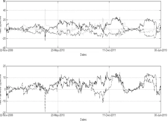
We can see in figure 3 that results for the entire period are still valid on a dynamic setting. In net terms, the M1 contract for each market has a positive volatility spillover and so transmits shocks, during all the period for the WTI and the NordPool. For the PJM and the Germany market it is also the case, but there exist some exceptional periods where the nearest contract receives volatility. The study of the net pairwise volatility spillover lead to the same conclusions. As for the static analysis, results for the Australian market are not exactly as expected. More precisely, the Q5 volatility spillover measure in net terms is often positive, indicating that this
(a) WTI
(c) PJM
(e) Australia
The first chart is for the net directional spillover. The solid line is for the nearest maturity, the dashed line for the intermediate maturity, and the dotted line for the most distant maturity. The second chart is for the net pairwise spillover against the nearest maturity. The solid line is for the intermediate maturity and the dashed line for the most distant maturity.
contract transmits volatility. We think this is because this contract has a very far away maturity which is not really impacted by current shocks.
To sum up, in this section we observe for each market except the Australian market, a transmission of prices shocks from the physical to the paper market. It is noteworthy that for some markets, it can exist periodically and rarely, some inverse process.
4
Going deeper in the analysis of the maturity impact
In this section we try to understand why the Samuelson hypothesis holds for our electricity futures markets. For this, we test different possible explanations: the impact of the volume or that of the inputs.
4.1 What about the trading volume?
As in Walls (1999), we want to study the link between the volume of trading and the maturity impact. The idea is to test if the Samuelson hypothesis is a phenomenon per se, or if it is a consequence of an increase in the trading volume during the life of a contract.
To do so we run a second regression, adding the daily volume as a control variable. The regression is the following:
σ2t = α + β1T T Mt+ β2V OLt+ εt
With T T Mt the number of days until expiration, and V OLt the daily volume in number of
contracts.
We consider the maturity impact as an independent phenomenon of the trading volume if β1 stays negative and statistically significant at the 1% level.
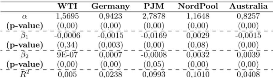
WTI Germany PJM NordPool Australia α 1,5695 0,9423 2,7878 1,1648 0,8257 (p-value) (0,00) (0,00) (0,00) (0,00) (0,00) β1 -0,0006 -0,0015 -0,0169 0,0029 -0,0015 (p-value) (0,34) (0,003) (0,00) (0,08) (0,00) β2 9E-07 0,0007 -0,0008 0,0032 0,0039 (p-value) (0,00) (0,00) (0,05) (0,00) (0,00) R2 0,005 0,0238 0,0993 0,1010 0,0408 Results of the following regression:
σ2t = α + β1T T Mt+ β2V OLt+ εt
Table 8: Linear regression with volume
The results, in Table 8, are not homogeneous. Indeed, the Samuelson hypothesis is robust to the addition of the volume for the German market, the PJM and the Australian market with, for each market, a β1 coefficient which stays negative and statistically significant. For these markets,
even if the volume explains part of the volatility (β2statistically significant), the maturity impact is independent of it. Whereas, it is not the case for the two other markets, because β1 coefficients of the WTI and the NordPool are no longer statistically significant. For the NordPool, the β1
Overall, we can note that the addition of the volume in the linear regression allows us to estimate a better model for all the markets but the PJM.
4.2 About indirect storability: Electricity prices and inputs prices
In this section we do not directly test if the Samuelson hypothesis holds for our markets thanks to their generation’s process, but we try to explicit the link that could exist between the behavior of electricity prices and prices of inputs used to produce it. Behind this, there is the idea of indirect storability of electricity used in pricing models of Routledge et al. (2001) [26], Aïd et al. (2009)[1] or Aïd et al. (2013) [2]. Our thought is the following: the electricity being produced by some inputs, price shocks on input markets should spread to electricity markets, and if it is the case, then the maturity impact could be a consequence of this.
To study this, we compute the volatility spillover measure of Diebold and Yilmaz (2012) [13], and we focus our attention on the PJM, for which the electricity is mainly produced using coal, natural gas and oil.
Here we use this framework to measure the volatility spillovers between PJM prices, WTI prices and natural gas prices. We want to study volatility spillovers between these three markets since the electricity traded in the PJM is produced for an important part by oil and natural gas. Indeed, oil and natural gas account respectively for 8% and 28% of the installed capacity in this area. We do not use coal prices since trading volumes are too low to have continuous time series of good quality.
To do so, we use the one month continuous time series (M1) for each market and we set the following parameters: as before, we use p = 4 lags for the VAR and H = 10 for the forecast error variance decompositions. These choices, somehow arbitrary, do not lead our results, since we have computed the volatility spillover measure using other parameters without significant changes.
We have two kind of results for our volatility spillover measure: we first compute this measure on the entire sample, and then, using a rolling window of ninety days.
Directional to Directional from Net Net Pairwise all others all others against PJM
PJM 8,55 13,48 -4,93
WTI 2,76 4,82 -2,06 0,47
Natural gas 15,96 8,97 6,99 -5,40 Net is "To all others-From all others". Net pairwise against PJM is "From PJM-To PJM"
Table 9: Volatility spillover on the entire period
At first, as shown in Table 9, on the entire time period the PJM and the WTI, with a net directional spillover of −4, 93 and −2, 06 are receiving volatility from other markets, while the natural gas delivers volatility to others. If we go deeper in the analysis for the PJM, we can see that, even if in net terms this market receives volatility, there exist a gross directional spillover of volatility from the PJM to all others markets. More precisely, the net pairwise volatility spillover shows that, in net terms, PJM delivers volatility to the WTI and receives volatility from the natural gas market.
(a) Net Directional Spillover
(b) Net Pairwise Spillover
The first chart is for the net directional spillover. The solid line is for the PJM, the dashed line for the WTI, and the dotted line for the natural gas. The second chart is for the net pairwise spillover against the PJM. The solid line is for the WTI and the dashed line for the natural gas.
That is, in net terms, the PJM and the WTI are most of the time receiving volatility from all other markets, whereas the natural gas market always delivers volatility to all others markets. And for net pairwise spillovers, most of the time, PJM seems to delivers volatility to the WTI, and receives volatility from the natural gas market .
Nevertheless, to be more accurate, we study more precisely these charts for the PJM. Actu-ally, the net directional spillover for this market increases during our time period being sometimes positive. Whereas on the same period, the net directional spillover for the WTI decreases and becomes negative. We think that there exist a link between this two dynamics, and the line for the net pairwise spillover between the PJM and the WTI confirms our thought. Indeed this line increases from −10 to 5 on our sample period.
Finally, with these results we can say that PJM prices seem to be connected to WTI and natural gas prices, and that at least a small part of the PJM prices’ behavior comes from input prices’ behavior. So far, we can’t provide more precise tests to explain the maturity impact on electricity markets regarding its inputs.
5
Conclusion
This article provides insights for the literature on commodity derivative markets, in several directions. First, it proposes a new empirical implication of the Samuelson Hypothesis and suggests the proper methodology to use it. Second, it enhances the knowledge about the dynamics of the futures prices in the four most important electricity futures markets, worldwide. Lastly, it confirms the links between this "new" commodity and other storable commodities through the notion of "indirect storability" and suggests the presence of directionality effects from the inputs to the electricity prices.This is interesting, as most of the models of the term structure of commodity prices rely on the storage theory (see for example Brennan (1958)[6], Brennan and Schwartz (1985)[7], and Cortazar and Schwartz (2003)[9]).
References
[1] R. Aïd, L. Campi, A. N. Huu, and N. Touzi. A structural risk-neutral model of electricity prices. International Journal of Theoretical and Applied Finance, 12(7):925–947, 2009.
[2] R. Aïd, L. Campi, and N. Langrené. A structural risk-neutral model for pricing and hedging power derivatives. Mathematical Finance, 23(3):387–438, July 2013.
[3] R. W. Anderson. Some determinants of the Volatility of Futures Prices. The Journal of Futures Markets, 3:249–266, 1985.
[4] H. Bessembinder, J. F. Coughenour, P. J. Seguin, and M. M. Smeller. Is there a term structure of futures volatilities? Reevaluating the Samuelson Hypothesis. The Journal of Derivatives, pages 45–58, 1996.
[5] F. Black and M. Scholes. The pricing of options and corporate liabilities. Journal of Political Economy, 3:637–654, 1973.
[6] M. J. Brennan. The Supply of Storage. American Economic Review, 48:50–72, 1958.
[7] M. J. Brennan and E. S. Schwartz. Evaluating Natural Resource Investments. Journal of Business, 58:135–157, 1985.
[8] M. J. Chambers and R. E. Bailey. A Theory of Commodity Price Fluctuations. Journal of Political Economy, 104(5):924–957, Oct. 1996.
[9] G. Cortazar and E. Schwartz. Implementing a Stochastic Model for Oil Futures Prices . Energy Economics, 25:215–238, 2003.
[10] A. Deaton and G. Laroque. On the Behaviour of Commodity Prices. Review of Economic Studies, 59(1):1–23, 1992.
[11] A. Deaton and G. Laroque. Competitive Storage and Commodity Price Dynamics. Journal of Political Economy, 104:896–923, 1996.
[12] F. X. Diebold and K. Yilmaz. Measuring financial asset return and volatility spillovers, with application to global equity markets. Economic Journal, 119:158–171, 2009.
[13] F. X. Diebold and K. Yilmaz. Better to give than to receive: Predictive directional mea-surement of volatility spillovers. International Journal of Forecasting, 28:57–66, 2012.
[14] H. N. Duong and P. S. Kalev. The samuelson hypothesis in futures markets: An analysis using intraday data. Journal of Banking & Finance, 32:489–500, January 2008.
[15] E. F. Fama and K. R. French. Commodity Futures Prices: Some Evidence on Forecast Power, Premiums and the Theory of Storage. Journal of Business, 60:55–73, 1987.
[16] E. F. Fama and K. R. French. Business Cycles and the Behavior of Metals Prices. Journal of Finance, 43:1075–1093, 1988.
[17] R. Huisman and M. Kilic. Electricity futures prices: Indirect storability, expectations, and risk premiums. Energy Economics, 34:892–898, April 2012.
[18] A. Jonckheere. A distribution-free k-sample test against ordered alternatives. Biometrika, 41:133–145, 1954.
[19] G. Koop, M. Pesaran, and S. Potter. Impulse response analysis in non-linear multivariate models. Journal of Econometrics, 74, 1996.
[20] D. Lautier and F. Raynaud. Statistical properties of derivatives: A journey in term struc-tures. Physica A, 390:2009–2019, 2011.
[21] M.B.Garman and M.Klass. On the estimation of security price volatilities from historical data. Journal of Business, 53(1):67–78, 1980.
[22] N. T. Milonas. Price variability and the maturity effect in futures markets. The Journal of Futures Markets, 3:443–460, 1986.
[23] M. Parkinson. The extreme value method for estimating the variance of the rate of return. Journal of Business, 53(1):61–65, 1980.
[24] M. Pesaran and Y. Shin. Generalized impulse response analysis in linear multivariate models. Economcis Letters, 58, 1998.
[25] B. R. Routledge, D. J. Seppi, and C. S. Spatt. Equilibrium Forward Curves for Commodities. Journal of Finance, 55:1297–1338, 2000.
[26] B. R. Routledge, C. S. Spatt, and D. J. Seppi. The "spark spread": An equilibrium model of cross-commodity price relationships in electricity. Tepper School of business, 2001.
[27] P. A. Samuelson. Proof that properly anticipated prices fluctuate randomly. Industrial Management Review, 6:41–49, 1965.
[28] T. Terpstra. The asymptotic normality and consistency of kendall’s test against trend when ties are present in one ranking. Indagationes Mathematicae, 14:327–333, 1952.
[29] W. D. Walls. Volatility, volume and maturity in electricity futures. Applied Financial Economics, 9:283–287, 1999.
[30] H. Working. The Theory of the Price of Storage. American Economic Review, 31:1254–1262, Dec. 1949.
A
Appendix
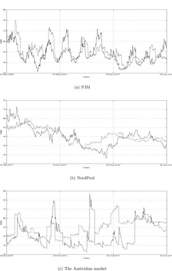
A.1 Continuous tim series of prices by maturity
(a) PJM
(b) NordPool
(c) The Australian market
The solid line is for the nearest maturity, and the dashed line is for the most distant maturity
A.2 Volatility of the closest-to-maturity time series
(a) WTI
(b) The German market
(d) NordPool
(e) The Australian market