Simple and extended Kalman filters : an application to term structures of commodity prices

SIMPLE AND EXTENDED KALMAN FILTERS: AN APPLICATION TO TERM STRUCTURES OF COMMODITY PRICES

DelphineLAUTIER and AlainGALLI

DelphineLAUTIER(*) is assistant professor at Cereg (University Paris IX) and associate

research fellow at Cerna (Ensmp).

Mailing Address: Cereg, Université Paris IX,

Place du Maréchal de Lattre de Tassigny, 75 775 Paris Cedex 16

E-mail: [email protected]

Telephone number and fax: 33 1 44 05 46 42 / 33 1 44 05 40 23

AlainGALLI is professor at Cerna (Ensmp)

Mailing address : Cerna, Ecole Nationale Supérieure des Mines de Paris,

60 boulevard Saint-Michel, 75 272 Paris Cedex 06

E-mail : [email protected]

Telephone number and fax: 33 1 40 51 90 91 / 33 1 44 07 10 46

Kalman Filters: An application to term structures of commodity prices

Abstract. This article presents and compares two different Kalman filters. These methods

provide a very interesting way to cope with the presence of non-observable variables, which is a frequent problem in finance. They are also very fast even in the presence of a large information volume. The first filter presented, which corresponds to the simplest version of a Kalman filter, can be used solely in the case of linear models. The second filter – the extended one – is a generalization of the first one, and it enables to deal with non-linear models. However, it also introduces an approximation in the analysis, whose possible influence must be appreciated. The principles of the method and its advantages are first presented. We then explain why it is interesting in the case of term structure models of commodity prices. Choosing a well-known term structure model, practical implementation problems are discussed and tested. Finally, in order to appreciate the impact of the approximation introduced for non-linear models, the two filters are compared.

S

IMPLE AND EXTENDED

K

ALMAN

F

ILTERS

:

AN APPLICATION TO TERM STRUCTURES OF COMMODITY PRICES

ABSTRACT: This article presents and compares two different Kalman filters. These methods provide a very interesting way to cope with the presence of non-observable variables, which is a frequent problem in finance. They are also very fast even for large data sets. The first filter presented, which corresponds to the simplest version of a Kalman filter, can be used solely for linear models. The second filter – the extended one – is a generalization of the first that can deal with non-linear models. However, it also introduces an approximation into the analysis, whose possible influence must be evaluated. The principles of the method and its advantages are first presented. We then explain why it is interesting in the case of term structure models of commodity prices. Choosing a well-known term structure model, practical implementation problems are discussed and tested. Finally, in order to appreciate the impact of the approximation introduced for non-linear models, the two filters are compared.

I.

T

HE

K

ALMAN FILTERS

:

A BRIEF INTRODUCTION1

The main principle of the Kalman filters is to use temporal series of observable variables in order to reconstitute the values of non-observable variables. In finance, the problem of non-observable variables arises for example with term structure models of interest rates, term structure models of commodity prices and with market portfolios in the capital asset pricing model. When associated with an optimization procedure, the Kalman filter provides a way to estimate the model parameters. Finally and most importantly, because it is very fast, the method is also interesting for large data sets.

There are different versions of Kalman filters2. The simple one is also the most famous and it is quite frequently used in finance nowadays3. Nevertheless, it is not suitable for nonlinear models. In that case, an extended filter can be used. However, the latter relies on an approximation, whose possible influence on the model performances needs to be assessed. Apart from this distinction, the two filters rely on the same principles.

The Kalman filter is an iterative process. The model has to be expressed in a state-space form characterized by a transition equation and a measurement equation4_{. This}

transition equation describes the dynamics of the state variables α~ , for which there are no empirical data. During the first step of the iteration – the prediction phase – this equation is used to compute the values of the non-observable variables at time t, conditionally on the information available at time (t-1). The predicted values α~_t/t−1 are then substituted into the measurement equation to determine the value of the measures y~ . The _t measurement equation represents the relationship linking the observable variables y~ with the non-observable α~ . In the second iteration step – or innovation phase – the innovation vt, which is the difference, at t, between the measure y~ and the empirical data yt t is

calculated. The innovation is used, in the third iteration step – or updating phase – to obtain the value of α~ conditionally on the information available at t. Once this t

calculation has been made, α~ is used to begin a new iteration. Thus, the Kalman filter _t makes it possible to evaluate the non-observable variables α~ , and it updates their value in each step using the new information.

This brief presentation explains why the Kalman filter is a very fast method. Indeed, to reconstitute the temporal series of the non-observable variables, only two elements are necessary: the transition equation and the innovation v. Because there is an updating phase in the iteration, very little information is needed.

The remainder of the paper is organized as follows. Section II presents the term structure models of commodity prices and explains why their use necessitates resorting to the Kalman filters. Section III explains how to apply the simple and the extended Kalman filters to a well-known model developed by Schwartz in 1997. Relying on the model performances, section IV compares the two filters and discusses some practical implementation problems. Section V concludes.

II.

T

HE TERM STRUCTURE MODELS OF COMMODITY PRICES

In this section, after describing some general features characterizing the term structure models of commodity prices, we present the model used for the comparison between the simple and the extended Kalman filters: Schwartz’s model.

General presentation

The term structure of commodity futures prices describes the relationships between the spot price and futures prices for different delivery dates. So it synthesizes all the information available in the market. Several term structure models have been proposed in the literature. Their objective is firstly to reproduce the observed futures prices as accurately as possible, and secondly to extend the curve for very long maturities, even for delivery dates which are not available in the market.

Term structure models borrow from the contingent claim analysis developed in a partial equilibrium framework for options and interest rates models. Relying on arbitrage reasoning, the development of a term structure model of commodity prices follows three successive steps: identification of the state variables, specification of their dynamics and extraction of the futures prices values from a differential valuation equation.

When only one state variable is used to explain the futures prices behaviour, as is the case, for example, in Brennan and Schwartz’s model (1985), this single factor is the spot price. Recognizing the limits of such a formulation, several models based upon two

state variables have been proposed (Schwartz, 1997; Hilliard and Reis, 1998; Lautier, 2000). In that case, the second factor is the convenience yield, which can be briefly defined as the comfort associated with the possession of physical stocks (Brennan, 1958). The introduction of a second state variable allows for richer shapes of curves and volatility structures. This improvement is however costly because the models are naturally more complicated. The difficulty arises from the increasing number of parameters and from the non-observable nature of the state variables. In fact, there are usually no empirical data for these two variables because there is generally a lack of reliable time series for the spot price5, and convenience yield is not a traded asset. Therefore, there is a need for a method like the Kalman filter.

Schwartz’s model

Schwartz’s model (1997) is a well-known term structure model of commodity prices. Three reasons lead to choose it. Firstly, it performs well. Secondly, it has an analytical solution, which simplifies the application of the Kalman filters. Thirdly, it allows for the use of a simple Kalman filter, provided some precautions are taken.

Schwartz’s model supposes that the spot price S and the convenience yield C can explain the behavior of the futures prices F. The dynamics of these state variables is:

(

)

[

]

⎩

⎨

⎧

+

−

=

+

−

=

C C S S

dz

dt

C

k

dC

Sdz

Sdt

C

dS

σ

α

σ

µ

)

(

with: κ, σS, σC >0

where: - µ is the drift of the spot price, -

σ

_S is the volatility of the spot price,

- dzS is an increment to a standard Brownian motion associated with S,

- α is the long run mean of the convenience yield, - κ is the speed of adjustment of the convenience yield, -

σ

_C is the convenience yield volatility,

As the storage theory showed, the two state variables are correlated because both the spot price and the convenience yield are an inverse function of the inventory levels. Nevertheless, as Gibson and Schwartz (1990) demonstrated, the correlation between these two variables is not perfect:

[

dz

dz

]

dt

E

_S

×

_C

=

ρ

where ρ is the correlation between the two Brownian motions associated with S and C. The convenience yield is mean reverting and is involved in the spot price dynamics. Mean reversion relies on the hypothesis that there is a level of stocks which satisfies the needs of industry under normal conditions. The behaviour of the operators in the physical market guarantees the existence of this normal level of stocks. When the convenience yield is low, the stocks are abundant and the operators sustain a high storage cost compared with the benefits related to holding the raw materials. So, if they are rational, they try to reduce these surplus stocks. Conversely, when the stocks are rare, the operators tend to reconstitute them.

The solution of the term structure model can be expressed in a risk neutral framework, using a Feynman-Kac solution. Therefore, the value of the futures prices can be written as:

( )

tT E

[

S

( )

T

]

F , = Qλ

where F(t,T) is the futures price at t for delivery at T, and

Q

_λ denotes the risk neutral probability6, which is dependent of an unknown value λ. The latter is the market price of convenience yield risk. The solution is:

( )

⎥ ⎦ ⎤ ⎢ ⎣ ⎡ + − − × = − τ κ κτ B e t C t S T t C S F( , , , ) ( ) exp ( )1 with:

( )

⎥ ⎥ ⎦ ⎤ ⎢ ⎢ ⎣ ⎡ ⎟⎟ ⎠ ⎞ ⎜⎜ ⎝ ⎛ − × ⎟⎟ ⎠ ⎞ ⎜⎜ ⎝ ⎛ − + + ⎥ ⎦ ⎤ ⎢ ⎣ ⎡ − × + ⎥ ⎥ ⎦ ⎤ ⎢ ⎢ ⎣ ⎡ × ⎟⎟ ⎠ ⎞ ⎜⎜ ⎝ ⎛ − + − = 2₂ 2 1 −₃2 2 1 ₂− 4 2 κ κ σ ρ σ σ κ α κ σ τ κ ρ σ σ κ σ α τ r e κτ e κτ B C C S C C S C ) ) _,

(

λ κ

)

α α)= − /

where : - r is the risk free interest rate, assumed constant, - τ = T - t is the maturity of the futures contract.

To assess the model’s performances, we first need the optimal values of the parameters, which can then be used to compute the estimated futures prices and to compare them with empirical data.

III.

A

PPLYING THE

K

ALMAN FILTERS

In this section, the way to transform Schwartz’s model into a state-space model is explained, for the simple and for the extended filters. Then, implementation problems are discussed.

Simple filter

The simple filter is suited for linear models. To apply it, the solution of Schwartz’s model must be expressed on a linear form:

(

)

( )

( )

τ κ κτ B e t C t S T t C S F( , , , ) =ln ( ) − ( )×1− − + ln

Letting G = ln(S), we also have7:

(

)

[

]

⎪⎩ ⎪ ⎨ ⎧ + − = + − − = C C S S S dz dt C k dC dz dt C dG σ α σ σ µ ) 2 1 ( 2

The state-space form of the model is the following. The transition equation is the expression, in discrete time, of the state variables dynamics. Using the same notation as before, this equation is:

t t t t t t t _R C G T c C G _{+ η} ⎥ ⎥ ⎦ ⎤ ⎢ ⎢ ⎣ ⎡ × + = ⎥ ⎥ ⎦ ⎤ ⎢ ⎢ ⎣ ⎡ − − − − 1 1 1 / 1 / ~ ~ ~ ~ , t = 1, ... NT where:

- ⎥ ⎥ ⎦ ⎤ ⎢ ⎢ ⎣ ⎡ ∆ ∆ ⎟ ⎠ ⎞ ⎜ ⎝ ⎛ − = t t c S

κα

σ

µ

2 2 1

- ∆t is the period separating 2 observation dates,

- _⎥ ⎦ ⎤ ⎢ ⎣ ⎡ ∆ − ∆ − = t t T κ 1 0 1

- R is the identity matrix, (2 × 2),

- ηt are errors that are uncorrelated with the previous values of the state variables, and

have no serial correlation :

E[ηt] = 0, and ⎥ ⎦ ⎤ ⎢ ⎣ ⎡ ∆ ∆ ∆ ∆ = = t t t t Var Q C C S C S S t 2 2 ] [

σ

σ

ρσ

σ

ρσ

σ

η

The measurement equation comes directly from the model pricing formula, which must also be discretized:

t t t t t t t C G Z d y +ε ⎥ ⎥ ⎦ ⎤ ⎢ ⎢ ⎣ ⎡ × + = − − − 1 / 1 / 1 / ~ ~ ~ _{, t = 1, ... NT} where :

- the ith _{line of the N dimensional vector of the observable variables} 1 /

~

− t t

y

is ln

( )

F~

( )

τ_i , with i= 1,..,N,

- d = [B(τi)] is the ith line of the d vector, with i = 1,..., N, and where:

⎥ ⎥ ⎦ ⎤ ⎢ ⎢ ⎣ ⎡ ⎟⎟ ⎠ ⎞ ⎜⎜ ⎝ ⎛ − × ⎟⎟ ⎠ ⎞ ⎜⎜ ⎝ ⎛ − + + ⎥ ⎦ ⎤ ⎢ ⎣ ⎡ _× − + ⎥ ⎥ ⎦ ⎤ ⎢ ⎢ ⎣ ⎡ × ⎟⎟ ⎠ ⎞ ⎜⎜ ⎝ ⎛ − + − = 2₂ 2 1 −₃2 2 1 ₂− 4 2 ) ( κ κ σ ρ σ σ κ α κ σ τ κ ρ σ σ κ σ α τ r e κτi e κτi B C C S C i C S C i ) ) α)=α−λ/κ

- Z =

[

1 , −H_i

]

is the ith _{line of the Z matrix, which is (N×2), with i = 1,...,N and} where: κ κτi e H_i − − =1

- εt is a white noise vector, (N×1), with no serial correlation:

In continuous time, the pricing equation of a term structure model does not involve any error term ε. The use of a Kalman filter leads to the introduction of this term, which is difficult to estimate. This term can be interpreted as follows. Firstly, it stands for market imperfections and arbitrage opportunities. Secondly, as the Kalman filter is a kind of inverse process, which is often unstable, it can be considered as a regularization term. Its addition leads to a distribution for

_y%

, which is the initial one, convoluted with a Gaussian kernel.

Extended filter

In an extended filter, the previous system matrices Z, T and R are replaced with non-linear functions depending on the state variables. So there is no need to linearize Schwartz’s model. The transition equation becomes:

t t t t t t t t t _{T S C R S C} C S _η ) ~ , ~ ( ) ~ , ~ ( ~ ~ 1 1 1 1 1 / 1 / − − − − − − _{= +} ⎥ ⎥ ⎦ ⎤ ⎢ ⎢ ⎣ ⎡ where: -

(

)

(

)

(

)

⎥⎥_⎦ ⎤ ⎢ ⎢ ⎣ ⎡ ∆ − + ∆ ∆ − ∆ + = − − − − − t C t t C t µ S C S T t t t t t _{κα κ} 1 ~ ~ 1 ~ ~ , ~ 1 1 1 1 1 -

(

)

_⎥ ⎦ ⎤ ⎢ ⎣ ⎡ = − − − 1 0 0 ~ ~ , ~ ₁ 1 1 t t t S C S R -

( )

_⎥ ⎦ ⎤ ⎢ ⎣ ⎡ = = ₂ 2 C C S C S S t Var Q σ σ ρσ σ ρσ σ η

The measurement equation becomes:

(

t t t t

)

t

t

t Z S C

y_{/ −1}= ~_/−1,~_{/ −1} +ε ~

where: Z

(

S~_t/t−1,C~_t/t−1

)

is an N dimensional vector, whose ith _{line is (i = 1,..., N):}

(

)

In the extended filter, as the transition and measurement equations are non-linear, there is no analytical formula for the conditional expectations. Therefore, the latter must be approximated. This approximation does not appear in the simple filter.

Implementation problems

Some difficulties must be overcome when using Kalman filters. First, some choices must be made to start the iterative process. Second, if the model has been expressed as the logarithm for the simple Kalman filter, some precautions must be taken. Third, the covariance matrix H influences the performances.

Starting the iterative process

To start the iterative process, initial values of the non-observable variables and of their covariance matrix are needed.

For the term structure models of commodity prices, the non-observable state variables are usually the spot price and the convenience yield. The nearest futures price is generally used as the spot price S, and the convenience yield C can be computed from the solution of Brennan and Schwartz’s model (1985). This solution requires the use of two observed futures prices, for delivery at T1 and at T2:

(

)

(

)

2 1 2 1) ln ( , , ) , , ( ln ) ( T T T t S F T t S F r t C − − − =

where T1 is the nearest delivery, and T2 is the next one.

The covariance matrix associated with the state variables must also be initialized. We choose a diagonal matrix with the spot price and the convenience yield variances on the diagonal. These variances were computed from the 30 first dates in the estimation period.

Analyzing the results of the simple filter

When the model is expressed in its logarithmic form in the case of the simple filter, some precautions must be taken to measure the model’s performances, because the innovations are computed with logarithms. A difficulty arises when the estimated and

empirical data are rebuilt. The relationship linking the estimations logarithm

~

y

_t/t−1 with the observations logarithm yt is the following:

R

y

y

_t

=

~

_t/t−1

+

σ

where σ is the standard error of the innovations and R is a gaussian residue. To be more precise, when the estimated logarithm is used to obtain the estimates themselves, the relationship between yt and

~

y

t/t−1 becomes :

R y

y

_e

_e

e

t

=

~t/t−1

×

σ

The expectation is then8 :

[ ] [ ]

~ 2 2 1 / σ

e

e

E

e

E

yt

=

ytt−

×

Therefore, a corrective term should be added to the estimations exponential. From a theoretical point of view, this is quite difficult, because the innovations variance is modified as soon as the parameters change. We nevertheless performed empirical tests, in order to measure this bias.

Measuring the performances

Another important choice must be made before initiating the iteration process, concerning the error covariance matrix H. This matrix is important because it is added to the innovations covariance matrix during the innovation phase. In the simple Kalman filter, the relationship between the innovations matrix Ft and the system matrix H is:

H Z ZP F_t = _t/t−1 '+

where Pt/t-1 is the covariance matrix of the non-observable variables and Z is a system

matrix included in the measurement equation.

During the next iteration phase, the inverse of the innovations matrix is used to update the non-observable variables and their covariance matrix:

(

)

⎪⎩ ⎪ ⎨ ⎧ − = + = − − − − − − 1 / 1 1 / 1 ' 1 / 1 / ˆ ' ˆ ˆ ~ ~ t t t t t t t t t t t t t t t t P Z F Z P I P v F Z P α α

So, the matrix H has an influence on the updated values of the non-observable variables. If its terms are too high, the model performances will be poor. Most of the time, this matrix is estimated relying on the variances and the covariance of the estimations database. We used this method in this article and we show how strongly this choice affects the empirical results.

IV.

C

OMPARISON BETWEEN THE TWO FILTERS

Comparing the performances of Schwartz’s model measured with the two filters makes it possible to assess the influence of the linearization on the results. In this section, the empirical data are first presented. Then the performance criteria are presented. Finally, the results are delivered and commented.

Data

The data used for the empirical study are daily crude oil settlement prices for the West Texas Intermediate (WTI) futures contracts negotiated on the New York Mercantile Exchange (Nymex) from 09/25/1995 to 01/14/2002. They have been arranged so that the first futures price maturity τ1 is the one month maturity, and that the second futures price

corresponds to the two months maturity τ2, ... Keeping the first observation of each group

of five, this daily data were transformed into weekly data. Four series of futures prices9 corresponding to maturities of one, three, six and nine were used to estimate the parameters, and to measure the model’s performance.

The interest rates are T-bill rates for a three months maturity. As they are supposed to be constant in the model, we used the mean of all the observations between 1995 and 2002.

Performances criteria

Two criteria were used to measure the model performances: the mean pricing error (MPE) and the root mean squared errors (RMSE).

The MPE is defined as follows:

( ) ( )

(

)

∑

= − = N n n F n F N MPE 1 , , ~ 1 _{τ τ}

where N is the number of observations, F~

( )

n,τ is the estimated futures price for maturity τ at the date n, and F

( )

n,τ is the observed futures price. The MPE is expressed in US dollars. It measures the estimation bias for one given maturity. If the estimation is good, the MPE should be very close to zero.

Using the same notation, the RMSE, expressed in US dollars, is, for a given maturity τ:

( ) ( )

(

)

∑

= − = N n n F n F N RMSE 1 2 , , ~ 1 _{τ τ}

When there is no bias, the RMSE can be considered as an empirical variance. It measures the estimation stability. This second criterion is considered as more representative because price errors can offset themselves and the MPE can be low even if there are strong deviations.

Empirical results

The estimation periods used to obtain the parameters are for the following periods: 09/25/95-05/11/98 and 05/18/98-10/15/01. After comparing the optimal parameters obtained with the two filters, we measure the model’s ability to represent the prices curves on the learning database and on an expanded one. Finally, the sensitivity of the results to the error covariance matrix are examined.

Optimal parameters

The optimal parameters were estimated with the simple and the extended filters10.

The results obtained for the two periods are represented in Tables 1 and 2. They lead to two remarks. Firstly, the parameters values change with the estimation period. This was observed in several earlier studies. Considering that the parameters are constant is rather

restrictive but it significantly reduces the complexity of the analysis. Secondly, the optimal parameters obtained with the two filters are different. During the first period, the optimal parameters obtained with the extended filter are usually higher than those associated with the simple filter. The principal differences concern the risk premium λ and the long run mean α . For the second period, the differences are lower, and the most important ones concern the volatilities of the state variables.

These differences show that the linearization has had a significant influence on the parameters. Nevertheless, the latter have always the same order size that those obtained by Schwartz in 1997 on the crude oil market and on different periods.

The model performances

A simple graphical analysis is first used to comment the model performances obtained with the two filters. Then the MPE and RMSE criteria are used to compare them. The results associated with the simple filter are also corrected for the logarithm. Lastly the innovations obtained with the two filters are compared.

Figure 1 represents the one-month futures prices observed during 1998-2001 and compares them with the futures prices estimated with the two filters. This graphic shows that firstly, the two filters, especially the simple one, attenuate the range of price fluctuations. We observed this phenomenon for the two study periods and for every maturity. Secondly, the Kalman filters can be used with extremely volatile data. During 1998-2001, the crude oil prices ranged from USD 11 per barrel to USD 37!

Tables 3 and 4 give the performances of Schwartz’s model, measured by the MPE and the RMSE criteria. Three conclusions can be drawn from these results. Firstly, the model is able to reproduce the prices curve quite precisely. The average MPE is always less than 18 cents per barrel and the RMSE is quite low, especially for the shorter period (1995-1998). Secondly, if the RMSE is the relevant criterion, then the simple filter is always more precise than the extended one. Thirdly, these measures always decrease

with maturity, which is consistent with Schwartz’s results on others periods. Nevertheless, Schwartz worked with longer maturities, and showed that the root mean squared error increases again for deliveries after 15 months.

To be rigorous, the model performances associated with the simple Kalman filter should be corrected when the model in expressed in terms of logarithms. Table 5 compares the performances obtained with and without correction. The results show that the correction slightly improves the performances. Therefore, in our case, the bias associated with the logarithm as a minor influence on the results, probably because the variance of the residuals is small for reasonable parameters values.

Finally, Figure 2 represents the behavior of the innovations for the one-month maturity and for the second study period. It shows that for both filters, the innovations tend to return to zero. The same observation can be made for the others maturities, likewise for both periods. The figure also shows that even if the MPE are low for the two filters, the pricing errors can be rather important at certain dates.

The performances analysis shows that there is clearly an impact of the linearization introduced in the extended filter. However, the most important is that, even if this impact is negative, the model’s ability to represent the prices curve is still good with an extended filter.

Expanding the database

The parameter estimates vary with the estimation periods. Hence, one question arises: how often is it necessary to recalculate the parameters? In order to answer that question, we used the parameters previously estimated to measure the model performances on an expanded database. We carried out these tests on two intervals of three months located in the prolongation of the estimation periods, namely 05/18/98 08/17/98 and 10/21/01 - 01/14/02. Tables 6 and 7 present our results. Two conclusions can be drawn.

Firstly, in 1998, the model is more precise with the extended filter. However, in 2001-2002, the simple filter gives again the best performances. Secondly, the model performances decrease strongly when the database is expanded. The RMSE and the MPE rise dramatically for the two periods. This phenomenon is particularly pronounced when the futures prices are volatile, during 2001-2002, and it will probably be even more marked as the database is increased. So, there is a strong incentive to recalculate the optimal parameters each time the model is used. This is not a major drawback, at least when there is an analytical solution for the model, because the estimation process is very fast.

Simulations

The last results presented are simulations showing how the choice of the system matrix H, which represents the errors in the measurement equation, affects the model performances. The first results presented in Table 8 (observations) are obtained with a matrix whose components are the variances and the covariance of the observations. This method is the most frequently used. The other performances (simulations) are carried out with artificially lowered matrices: in simulations 1 to 4, H was multiplied by (1/2), (1/16), (1/160), and (1/1600). For these tests, we retained the period 1998-2001 because it is characterized by especially volatile data.

Table 8 illustrates that, when the matrix components are lowered, the model performances improve strongly: from the initial performances to the fourth simulation, the RMSE is almost divided by two. However, comparing the third and the fourth simulation also shows that there is a limit to the improvement. Figure 3 summarizes the main results of these simulations.

Kalman filters are powerful tools suitable for use in many fields in finance, because they are fast even for large data sets and they can handle unobservable variables. Moreover, they can be used for linear as well as non-linear models, even if the models have no analytical solutions.

The main conclusions of this article are the following. Firstly, the approximation introduced in the extended Kalman filter due to linearizing the model, clearly influences the model performances: the extended filter generally leads to less precise estimates than the simple one. Nevertheless, as the difference between the two filters is quite small, the extended filter is still acceptable in our case. So, the approximation is not a real problem until the model becomes highly nonlinear. Secondly, the system matrix containing the errors of the measurement equation affects the model performances and can be used to obtain more precise results. Thirdly, as far as the term structure models of commodity prices are concerned, the parameters are not constant in time and should be recomputed regularly. This can become a problem if the model has no analytical solution, because of the computing time.

In order to improve the use of the Kalman filters, some further studies could be considered. For example, in the matrix representing the errors in the measurement equation (which is most of the time estimated with variances and covariance), we could also try to use variograms. This tool borrowed from geostatistics are used to describe spatial or temporal correlation11. More precisely, a variogram models the variation of the correlations between a pair of points of the same variable as a function of the spatial or temporal distance. Another improvement could be done concerning the analysis of the bias associated with the logarithms in the simple Kalman filter. To reduce this bias, variance minimization could be included in the iterative process used to estimate the optimal parameters. Lastly, to face the problem of time varying parameters in term structure models of commodity prices, one could study the sensitivity of the estimated futures prices to the parameters.

ACKNOWLEDGMENTS

We whish to thank the French Institute of Energy (Institut Français de l’Energie) for its support, and TotalFinaElf, who provided us with the empirical data used in this study. REFERENCES

Anderson, B.D.O. and Moore, J.B. (1979) Optimal filtering, Englewood Cliffs, Prentice Hall.

Babbs, S.H. and Nowman, B.K. (1999) Kalman filtering of generalized Vasicek term structure models, Journal of Financial and Quantitative Analysis, 34, 115--130.

Brennan, M.J. (1958) The supply of storage, American Economic Review, 47, 50--72. Brennan, M.J. and Schwartz, E.S. (1985) Evaluating natural resource investments, Journal of Business, 58, 135--157.

Fouque, J.P, Papanicolaou, G. and Sircar, K. (2000) Derivatives in financial markets with stochastic volatility, Cambridge University Press.

Gibson, R. and Schwartz, E.S. (1990)Stochastic convenience yield and the pricing of oil contingent claims, Journal of Finance, 45, 959--975.

Harvey, A.C., (1989) Forecasting, structural time series models and the Kalman filter, Cambridge University Press.

Hilliard, J.E. and Reis, J. (1998) Valuation of commodity futures and options under stochastic convenience yield, interest rates, and jump diffusions in the spot, Journal of Financial and Quantitative Analysis, 33, 61--86.

Horsnell, P and Mabro, R. (1993) Oil markets and prices, Oxford University Press. Javaheri, A., Lautier, D. and Galli, A. (2003) Filtering in finance, Willmott magazine, 5, (forthcoming).

Lautier, D. and Galli, A. (2002) Report on term structure models of commodity prices: elaboration and improvement, French Institute of Energy Research.

Lautier, D. (2000) La structure par terme des prix des commodités: analyse théorique et applications au marché pétrolier, Ph. D thesis, University Paris IX.

Schwartz, E.S. (1997) The stochastic behavior of commodity prices: implications for valuation and hedging, Journal of Finance, 52, 923--973.

Figure 1. Estimated and observed futures prices for the one-month’s maturity, 1998-2001

10

15

20

25

30

35

18/05 /98 18/07/9818/09/9818/11/9 8 18/01 /99 18/03/9918/05 /99 18/07/9918/09/9918/11/9918/01 /00 18/03/0018/05/0018/07 /00 18/09 /00 18/11/0018/01/0118/03/0118/05 /01 18/07 /01 18/09 /01

($/b)

Figure 2. Innovations, 1998-2001

-7

-6

-5

-4

-3

-2

-1

0

1

2

3

4

5

6

7

18/05 /98 18/07 /98 18/09 /98 18/11 /98 18/01 /99 18/03 /99 18/05 /99 18/07 /99 18/09 /99 18/11 /99 18/01 /00 18/03 /00 18/05 /00 18/07 /00 18/09 /00 18/11 /00 18/01 /01 18/03 /01 18/05 /01 18/0 7/01 18/0 9/01

($/b)

Figure 3. One-month’s futures prices observed and estimated, 1998 - 2001

10,00

15,00

20,00

25,00

30,00

35,00

18/05/98

18/07/98

18/09/98

18/11/98

18/01/99

18/03/99

18/05/99

18/07/99

18/09/99

18/11/99

18/01/00

18/03/00

18/05/00

18/07/00

18/09/00

18/11/00

18/01/01

18/03/01

18/05/01

18/07/01

18/09/01

($/b)

Observed futures prices for a one month's maturity

Estimated futures prices for a one month's maturity with a matrix H corresponding to the observations.

Estimated futures prices for a one month maturity and an artificially lowered matrix (Simulation 4)

Table 1. Optimal parameters, 1995-1998

Simple filter Extended filter

Parameters Gradients Parameters Gradients

Drift : µ 0.142741 0.001629 0.192335 0.000083

Speed of adjustment : κ 1.969842 -0.000265 2.023929 0.000114

Spot price volatility : σS 0.241347 0.000177 0.228553 0.000339

Long run mean : α 0.098906 0.001271 0.149024 0.001422

Convenience yield volatility : σC 0.400676 -0.001242 0.383852 0.000053

Correlation coefficient : ρ 0.967136 -0.000031 0.973072 -0.000001

Table 2. Optimal parameters, 1998-2001

Simple filter Extended filter

Parameters Gradients Parameters Gradients

Drift : µ 0.379926 0.000497 0.352014 -0.001178

Speed of adjustment : κ 1.59171 -0.003631 1.258133 0.000628

Spot price volatility : σS 0.263525 -0.000448 0.320235 -0.000338

Long run mean : α 0.252260 -0.012867 0.232547 0.004723

Convenience yield volatility : σC 0.237071 -0.000602 0.288427 -0.001070

Correlation coefficient : ρ 0.938487 -0.001533 0.969985 0.000008

Table 3. The model’s performances with the simple and the extended filters, 1995-1998

Simple filter Extended filter

Maturity MPE RMSE MPE RMSE

1 month -0.063 1.2769 0.0775 1.3972 3 months 0.1064 1.1804 0.2145 1.3011 6 months 0.1453 1.0142 0.2235 1.0861 9 months 0.1419 0.8468 0.2029 0.8812 Average 0.0827 1.0796 0.1796 1.1664 Unit: USD/b.

Table 4. The model’s performances with the simple and the extended filters, 1998-2001

Simple filter Extended filter

Maturity MPE RMSE MPE RMSE

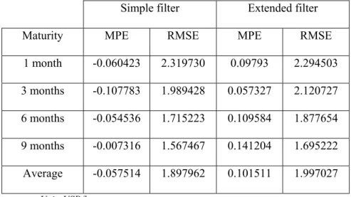
1 month -0.060423 2.319730 0.09793 2.294503 3 months -0.107783 1.989428 0.057327 2.120727 6 months -0.054536 1.715223 0.109584 1.877654 9 months -0.007316 1.567467 0.141204 1.695222 Average -0.057514 1.897962 0.101511 1.997027 Unit: USD/b.

Table 5. The simple filter with and without corrections for the logarithm, 1998-2001

Simple filter Simple filter corrected Maturity MPE RMSE MPE RMSE

1 month -0.060423 2.319730 0.065644 2.314178 3 months -0.107783 1.989428 0.006419 1.981453 6 months -0.054536 1.715223 0.026010 1.709931 9 months -0.007316 1.567467 0.061301 1.564854 Average -0.057514 1.897962 0.036637 1.892604 Unit: USD/b.

Table 6. The performances with a 3 months’ extrapolation, 1998

Simple filter Extended filter

Maturity MPE RMSE MPE RMSE

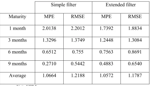
1 month 2.0138 2.2012 1.7392 1.8834 3 months 1.3296 1.3749 1.2448 1.3084 6 months 0.6512 0.755 0.7563 0.8691 9 months 0.2710 0.5442 0.4883 0.6540 Average 1.0664 1.2188 1.0572 1.1787 Unit: USD/b.

Table 7. The performances with a 3 months’ extrapolation, 2001-2002

Simple filter Extended filter

Maturity MPE RMSE MPE RMSE

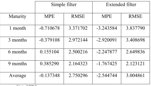
1 month -0.710678 3.371702 -3.243584 3.837790 3 months -0.379108 2.972144 -2.920091 3.408698 6 months 0.155104 2.500216 -2.247877 2.649836 9 months 0.385290 2.164323 -1.767425 2.123121 Average -0.137348 2.750296 -2.544744 3.004861 Unit: USD/b.

Table 8. Simulations with different system matrices

1 month 3 months 6 months 9 months Average Observations MPE RMSE 0.0979 2.2945 0.0573 2.1207 0.1096 1.8777 0.1412 1.6952 0.1015 1.9970 Simulation 1 MPE RMSE 0.0013 1.8356 0.0935 1.5405 0.1501 1.2478 1.6506 2.6602 0.4739 1.8210 Simulation 2 MPE RMSE 0.0073 1.4759 0.0152 1.1686 0.0612 0.9386 0.0137 0.8317 0.0244 1.1037 Simulation 3 MPE RMSE 0.0035 1.3812 -0.003 1.0950 0.0383 0.8647 0.0005 0.7499 0.0105 1.0227 Simulation 4 MPE RMSE 0.0131 1.3602 0.0067 1.0919 0.0415 0.8697 0.0075 0.7591 0.0172 1.0202 Unit: USD/b.

APPENDIX: THE SIMPLE AND THE EXTENDED KALMAN FILTERS

This appendix presents the simple and the extended Kalman filters, and explains how to estimate the model parameters.

1. The simple Kalman filter12

The state-space form model, in the simple filter, is characterized by the following equations:

• Transition equation: α_t/t−1=Tα_t−1+c+Rη_t

where αt is the m-dimensional vector of non-observable variables at t, also called state

vector, T is a matrix (m × m), c is an m-dimensional vector, and R is (m × m) • Measurement equation: y_t/t−1=Zα_t/t−1+d +ε_t

where y_t/t−1 is an N-dimensional temporal series, Z is a (N×m) matrix, and d is an m-dimensional vector.

t

η

and

ε

_tare white noises whose dimensions are respectively m and N. They are supposed to be normally distributed, with zero mean and with Q and H as covariance matrices:

E

[ ]

η

_t

=

0

,

Var

[ ]

η

_t

=

Q

[ ]

_t

=

0

E

ε

,

Var

[ ]

ε

_t

=

H

The initial value of the system is supposed to be normal, with mean and variance:

[ ]

α0 =α~0

E ,

Var

[ ]

α

₀

=

P

₀

If α~ is a non biased estimator of _t αt, conditionally on the information available at

t, then: E_t

[

α_t −α~ =_t

]

0

As a consequence, the following expression13 defines the covariance matrix P

t :

(

)(

)

[

~_{t t} ~_{t t} '

]

t t E P = α −α α −α

During one iteration, three steps are successively tackled: prediction, innovation and updating.

• Prediction : ⎩ ⎨ ⎧ + = + = − − − − ' ' ~ ~ 1 1 / 1 1 / R Q R T P T P c T t t t t t t α α

where α~_t/t−1 and Pt / t-1 are the best estimators of αt/t-1 and Pt/t-1 , conditionally on the

information available at (t-1). • Innovation : ⎪ ⎩ ⎪ ⎨ ⎧ + = − = + = − − − − H Z ZP F y y v d Z y t t t t t t t t t t t ' ~ ~ ~ 1 / 1 / 1 / 1 / α

where ~y_t/t−1 is the estimator of the observation yt conditionally on the information

available at (t-1), and vt is the innovation process, with Ft as a covariance matrix.

• Updating : ⎪⎩ ⎪ ⎨ ⎧ − = + = − − − − − − 1 / 1 1 / 1 1 / 1 / ) ' ( ' ~ ~ t t t t t t t t t t t t t P Z F Z P I P v F Z P α α

The matrices T, c, R, Z, d, Q, and H are not time dependent in the simplest case that we consider in this article. They are the system matrices associated with the state-space model.

2. The extended Kalman filter14

When the model is non-linear, it is generally impossible to obtain an optimal estimator for the non-observable variables. The simplest way to handle non-linearity is to linearize the equations. This is the idea behind the extended Kaman filter. However, because of this linearization at each step, it may happen that the approximate solution diverges on the long run.

In the non-linear case, the measurement and transition equations of the state-space form model are the following:

• Transition equation: α_t/t−1=T(α_t−1)+R(α_t−1)η_t

where αt/t-1 is the m-dimensional state vector at t,

T

(

α

t−1

)

and

R

t

(

α

t−1

)

are non linear functions, from Rm

_to

_Rm_{, depending on the values of the state variables at (t-1).}

where y_t/t−1represents an N dimensional temporal series, and Z(α_t/t−1) is a non-linear function, from RN

_to

_RN_{, of the non-observable variables.}

As was the case in the simple filter, the two processes εt and ηt are supposed to be

normally distributed, with zero mean, with H and Q as covariance matrices, and Pt is the covariance matrixassociated with α~ . _t

• Linearization:

If the functions Z(α_t/t−1) et

T

(

α

_t−1

)

are smooth enough, it is possible to compute their first order development around respectively α~_t/t−1and α~_t−1, where α~_t/t−1 is the expectation of α~ , conditionally on the information available at (t-1), and _t α~_t−1 is the value obtained for the state variable in (t-1), at the end of the updating phase. The state-space linearized model is then:

⎪⎩ ⎪ ⎨ ⎧ + ≈ + ≈ − − − − t t t t t t t t t Z y R T ε α η α α 1 / 1 / 1 1 / ˆ ˆ ˆ where : 1 / 1 / ~ ' 1 / 1 / ) ( ˆ − −= − − = t t t t t t t t Z Z α α δα α δ , 1 1 ~ ' 1 1) ( ˆ − − = − − = t t t t T T α α δα α δ , Rˆ=R(α~_t−1)≈R(α_t−1)

In the extended version, the three iteration steps are the following:

• Prediction: ⎪⎩ ⎪ ⎨ ⎧ + = = − − − − ' ˆ ˆ ' ˆ ˆ ) ~ ( ~ 1 1 / 1 1 / R Q R T P T P T t t t t t t α α

where α~_t/t−1and Pt/t-1 are the estimators for αt/t-1 and Pt/t-1, conditionally on the

information available at (t-1). • Innovation: ⎪ ⎩ ⎪ ⎨ ⎧ + = − = = − − − H Z P Z F y y v Z y t t t t t t t t t t t t ' ˆ ˆ ~ ) ~ ( ~ 1 / 1 / 1 / α

where ~y_t/t−1is the estimation of the observation yt, conditionally on the information

• Updating:

(

)

⎪⎩ ⎪ ⎨ ⎧ − = + = − − − − − − 1 / 1 1 / 1 ' 1 / 1 / ˆ ' ˆ ˆ ~ ~ t t t t t t t t t t t t t t t t P Z F Z P I P v F Z P α α

In the most simple case, the functions Z(α_t/t−1),

T

(

α

_t−1

)

, and R(α_t−1), just as the covariance matrices H and Q, are not time dependent. Z(α_t/t−1),

T

(

α

_t−1

)

and

) ( _t−1

Rα are the system functions. H and Q are the system matrices.

3. The parameters estimation

Suppose that the non-observable variables and the errors are normally distributed. Then we can use the maximum likelihood to estimate the model parameters, which are supposed to be constant. We have therefore to maximize the likelihood, or equivalently to minimize its logarithm. This implies that we must compute the likelihood for many parameters values. For that purpose, we used each time the Kalman filter with the current value of the parameters, and we computed, at each iteration, the logarithm of the likelihood function for the innovation vt :

t t t t

v

F

v

dF

n

t

l

⎟

×

Π

−

−

×

×

⎠

⎞

⎜

⎝

⎛

−

=

_'

−1

2

1

)

ln(

2

1

)

2

ln(

2

)

(

log

where Ft is the covariance matrix associated with the innovation vt, and dFt its

determinant15_{. In our case, the measurement equation admits continuous partial}

derivatives of first and second order on the parameters. Therefore, we can use a more powerful minimization method. Once the optimal parameters have been obtained, the Kalman filter is used, for the last time, to reconstitute the non-observable variables and the measure y~ .

1 _{A more precise presentation of the filters and of the parameters estimation procedure can be found in the}

appendix.

2 _{For a brief presentation of more complex non-linear filters or non Gaussian methods see for example}

Javaheri et al. (2003).

3 _{See for example Schwartz (1997) or Babbs and Nowman (1999).}

4 _{There is more than one state-space form for certain models. Then, because some of them are more stable}

than the others, the choice of one specific representation is important.

5 _{This is especially true for the American crude oil market, as Horsnell and Mabro (1993) explained it.} 6 _{In the case of term structure models of commodity prices, certain conditions must be respected in order to}

obtain a unique risk-neutral probability. For more details on that remark, see for example Lautier (2000). 7 _{In this article, we used the historical probability for the state variables dynamics. However, the futures price}

being expressed in a risk-neutral framework, it is possible to use this probability for the state variables. This method reduces the number of parameters: the drift µ and the risk premium λ disappear. It also induces a loss of information, because we must directly estimate the parameter α).



8

e

~yt/t−1_and

e

σR _{are not correlated.}

9 _{Thus N = 4 in our case.}

10 _{Optimizations have been made with a precision of 1}e_{-5 on the gradients. For the two filters and the two}

periods, we used the same parameters values to initiate the optimization. These values are: µ = 0.1; κ = 0.5 ; σS = 0.3 ; α = 0.1 ; σC = 0.4 ; ρ = 0.5 ; λ = 0.1.

11_{They were already used in finance, in another context, by Fouque, Papanicolaou and Sircar (2000).} 12 _{Harvey (1989) inspired this presentation.}

13

(

~

)

_'

t t α

α − is the transposed matrix of

(

α~_t −α_t

)

.

14 _{Harvey (1989) and Anderson and Moore (1979) inspired this presentation.} 15 _{The value of logl(t) is corrected when dF}