Quantification de la valeur ajoutée par le premier grand ensemble de simulations de changement climatique à haute résolution sur le Québec

(1)

QUANTIFICATION DE LA VALEUR AJOUTÉE PAR LE PREMIER GRAND ENSEMBLE DE SIMULATIONS DE CHANGEMENT CLIMATIQUE À HAUTE

RÉSOLUTION SUR LE QUÉBEC

MÉMOIRE

PRÉSENTÉ

COMME EXIGENCE PARTIELLE,

DE LA MAÎTRISE EN SCIENCES DE L'ATMOSPHERE

PAR

MOUSSA BOPP

(2)

UNIVERSITÉ DU QUÉBEC À MONTRÉAL Service des bibliothèques

Avertissement

La diffusion de ce mémoire se fait dans le respect des droits de son auteur, qui a signé le formulaire Autorisation de reproduire et de diffuser un travail de recherche de cycles supérieurs (SDU-522 – Rév.01-2006). Cette autorisation stipule que «conformément à l’article 11 du Règlement no 8 des études de cycles supérieurs, [l’auteur] concède à l’Université du Québec à Montréal une licence non exclusive d’utilisation et de publication de la totalité ou d’une partie importante de [son] travail de recherche pour des fins pédagogiques et non commerciales. Plus précisément, [l’auteur] autorise l’Université du Québec à Montréal à reproduire, diffuser, prêter, distribuer ou vendre des copies de [son] travail de recherche à des fins non commerciales sur quelque support que ce soit, y compris l’Internet. Cette licence et cette autorisation n’entraînent pas une renonciation de [la] part [de l’auteur] à [ses] droits moraux ni à [ses] droits de propriété intellectuelle. Sauf entente contraire, [l’auteur] conserve la liberté de diffuser et de commercialiser ou non ce travail dont [il] possède un exemplaire.»

(3)

Ce travail a été réalisé à Ouranos, consortium sur la climatologie régionale et l'adaptation aux changements climatiques sous la direction du professeur René LAPRISE et du docteur Martin LEDUC.

Au terme de ce projet, je tiens à remercier le docteur Martin LEDUC. Vous vous êtes montré à l'écoute et TRÈS patient tout au long de la réalisation de ce travail. Je tiens à vous dire que ce projet est avant tout pour moi un aboutissement et un épanouissement personnels auxquels vous avez pris une grande part. J'ai beaucoup apprécié ce travail avec vous.

Je souhaite aussi exprimer ·ma gratitude et toute ma reconnaissance au professeur René LAPRISE. Je suis reconnaissant pour tous vos conseils et remarques durant toute ma formation en Maîtrise.

J'adresse aussi des chaleureux remerciements à Sébastien Biner. Votre aide et contribution ont été bénéfiques pour la réussite de ce projet.

Enfin un grand Merci au Centre ESCER (Étude de la Simulation du Climat à l'Échelle Régional) de l'Université du Québec à Montréal, à Ouranos et au programme MITACS pour leur soutien financier.

(4)

TABLE DES MATIÈRES

LISTE DES FIGURES ... V

LISTE DES TABLEAUX ... vii

LISTE DES ABRÉVIATIONS, DES SIGLES ET DES ACRONYMES ... viii

RÉSUMÉ ... x

CHAPITRE I Introduction ... 1

CHAPITRE II QUANTIFYING THE ADDED V ALDE BY THE FIRST LARGE ENSEMBLE OF HIGH-RESOLUTION CLIMATE-CHANGE SIMULATIONS OVER QUÉBEC ... 8

2.1 Abstract ... 9

2.2 Introduction ... 10

2.3 Data ... 14

2.3.1 CanESM2 and CRCM5 model simulations ... 14

2.3.2 Choice of observation data ... 16

2.4 Methodology ... 17

2.4.1 Definition of added value ... 17

2.4.2 Interpolation on a common grid ... 18

2.4.3 Spatial decomposition into large and small scales ... 19

2.4.4 Spectral analysis ... 20

2.5 Results ... ... 21

2.5.1 Added value by the ensemble size ... ... : ... ,.21

2.5 .2 Added value by high resolution ... 23

2.6 Discussion and conclusions ... 28

(5)

TABLEAUX ... 51

CHAPITRE III Conclusion ... 53

ANNEXE Ergodicity of the large ensemble ... 58

(6)

LISTE DES FIGURES

Figure Page

2.1 Structure of the ClimEx project simulations ... 35 2.2 Topography of the MRCC5 ... 36 2.3 Ensemble-average monthly mean precipitation as a fonction of the number

of members for the months of July 2000 (lines 1 and 2) and January 2000 (lines 3 and 4) ... 37 2.4 Ensemble-average monthly mean temperature as a fonction of the number

ofmembers for the months of July 2000 (line 1) and January 2000 (line 2)

2.5 Average precipitation variance spectrum ( dashed line) and spectral variance of the ensemble-average precipitation ( continuous lines) as a

38

fonction of the number of members for July 2000 ... 39 2.6 Same _as figure 2.5 but for the month of January 2000 ... 40 2.7 Average temperature variance spectrum (dashed line) and spectral

variance of the ensemble-average of monthly-mean temperature (continuous lines) as a fonction of the number of members for July 2000. 41 2.8 Same as figure 2. 7 but for the month of January 2000 ... 42 2.9 Climate averages of January temperature between 1980-2010 for RCM

(left), GCM (middle) and CRU (right) ... 43 2.10 Climate averages of July precipitation between 1980-2010 for RCM (left),

(7)

2.11 Summer mean precipitation interpolated on the RCM grid with linear methods (linel). Cubic (line2) and nearest neighbour (line3) ... 45 2.12 Large and small scale decomposition ofprecipitation for July 2001 for the

RCM (line 1), GCM (line 2) and GPCP (line 3) ... 46 2.13 Spectral variance of the precipitation of the 50 individual members for the

month of July 2010 for the RCM (blue) and for the GCM (red). The black curve represents the variance spectrum of the July 2010 precipitation for the GPCP ... ,... 47 2.14 Analysis sub-domain centred over the Great Lakes .. ... .. ... ... 48 2.15 Spectral variance of montly mean precipitation from July for the years 1998 to

2012 for the RCM, CRU, GCM, Daymet and RCM_ERA ... 49 A. l Mean and standard deviation of July precipitation for 1955, 1956 and 1957

for kda, kdb and kdc members... 59 A.2 Mean and standard deviation of July temperature for 1955, 1956 and 1957

(8)

LISTE DES TABLEAUX

Tableau Page

(9)

CanESM2 Canadian Earth System Madel

CLASS Canadian LAnd Surface Scheme

CRCM5 Canadian Regional Climate Madel, version 5

· CRU Climatic Research Unit

ECCC Environnement et Changement climatique Canada

ESCER (Centre pour l') - étude et la simulation du climat à l'échelle régionale

GEM Global Environment Multiscale

GCM Global Climate Madel.

GPCP Global Precipitation Climatology Project

MCG Modèle de Circulation Générale

MRC Modèle Régional du Climat

MRCC5 Modèle Régional Canadien du Climat, Version 5

(10)

(11)

Les modèles régionaux du climat (MRC) ont été développés pour mieux représenter le climat à l'échelle régionale par rapport aux modèles climatiques globaux (MCG), l'amélioration de la résolution des MRC devant en principe permettre une meilleure représentation des processus atmosphériques. Dans ce projet, la valeur ajoutée du grand ensemble de 50 simulations à haute résolution (12 km) du Modèle Régional Canadien du Climat (MRCC5) piloté par le modèle global canadien (CanESM2), est évaluée à

différentes échelles spatiales. L'objectif de ce projet est de quantifier deux aspects de la valeur ajoutée: d'abord, en fonction du nombre de membres de l'ensemble; deuxièmement, la valeur ajoutée reliée à la haute résolution du MRCC5 par rapport CanESM2 et aux données d'observation. La méthodologie consiste d'abord à étendre la définition de la valeur ajoutée au cas d'un grand ensemble, en termes de sa capacité à

échantillonner la variabilité interne du système climatique à l'échelle régionale. La deuxième partie de la méthodologie comprend trois grandes étapes visant à valider les petites échelles ajoutées par le MRCC5 par rapport au CanESM2 et aux données d'observation. Pour ce faire, une interpolation est effectuée pour comparer ~es trois ensembles de données sur une grille commune. Une décomposition spatiale est ensuite appliquée pour évaluer la valeur ajoutée des différents groupes d'échelles spatiales. Enfin, une analyse spectrale est utilisée pour quantifier la valeur ajoutée en fonction de l'échelle spatiale. Les résultats montrent que la valeur ajoutée est plus visible dans les précipitations puisque cette variable contient une proportion plus élevée d'échelles fines, et donc une pente spectrale moins raide par rapport à la température. Nous avons également noté que la valeur ajoutée est plus importante près des Grands Lacs, des côtes et des montagnes; ces régions étant beaucoup mieux représentées dans le MRCC5

(12)

XI

à haute résolution que dans le CanESM2. De plus, la comparaison de ces deux modèles avec les observations a montré que les simulations du MRCC5 sont généralement plus proches des observations que celles du CanESM2.

(13)

INTRODUCTION

· Pour quantifier les impacts et s'adapter face aux changements climatiques, les scientifiques s'appuient souvent sur des s.imulations climatiques générées par des modèles numériques tels que les modèles climatiques globaux (MCG). Un MCG est l'outil principal et le plus complet pour étudier le climat actuel et futur. Il contient des composantes qui permettent de décrire les processus atmosphériques, terrestres et océaniques pouvant influencer le climat à des échelles de temps allant de quelques heures à des centaines, voire des milliers d'années (Di Luca et al. 2015). Les MCG ciblent donc les caractéristiques à grandes échelles du système climatique. La fiabilité de ces modèles est très importante car les attentes des décideurs en matière de projections climatiques sont très élevées pour répondre aux besoins de la communauté. Le réalisme des modèles climatiques à reproduire correctement le climat est aussi important car une cascade d'incertitude sera transmise et amplifiée à chaque étape de la chaine de décision (Wilby et Dessai 2010). Cependant, en raison de la complexité • des processus physiques, de la longueur des simulations, des variétés de forçages externes, les modélisateurs sont forcés d'utiliser des mailles de calcul très grossières pour les MCG par rapport aux modèles numériques de prévision météorologiques. La résolution des MCG est ainsi limitée à des centaines de kilomètres; ce qui empêche malheureusement une représentation détaillée des processus climatiques à fines échelles.

(14)

2

Ainsi, pour avoir des données climatiques plus adéquates à l'échelle locale avec une meilleure résolution, des modèles régionaux du climat (MRC) ont été développés depuis plus de 30 ans (Dickinson et al.1989). Le but des MRC est donc d'étendre l'utilité de la modélisation climatique en fournissant des informations plus détaillées et qui sont fondamentales pour les projections des changements climatiques. Il y' a donc deux motivations au développement des MRC. Tout d'abord, il existe une multitude de phénomènes climatiques dont les structures varient localement, en raison des contrastes dans les propriétés de la surface terrestre et des caractéristiques météorologiques à petites échelles. Deuxièmement, il est nécessaire d'avoir des informations sur ces phénomènes pour l'évaluation locale du changement climatique et les études d'impacts. La résolution améliorée des MRC est censée permettre une discrétisation plus précise des équations et une meilleure représentation de l'hétérogénéité des forçages de surface comme les contrastes terre-mer, l'orographie, la distribution des lacs et des rivières, les types de canopée de la végétation et les propriétés des sols. Les variations spatiales et temporelles des caractéristiques de la surface impriment donc une signature sur le climat régional qui est mieux représenté par un MRC à haute résolution. Les travaux de Di Luca et al. (2013) et Prommel et al. (2009) ont montré par exemple que dans les régions de topographie complexe, l'utilisation d'un maillage plus fin permet de résoudre les gradients de température près de la surface à plus petite échelle en raison de l'orographie mieux décrite et de la variation générale de la température de l'air avec l'altitude. D'autre part, certains MRCs sont couplés avec les lacs, mers et océans cotiérs la glace océanique, la végétation etc (Rinke et al. 2003, Doscher et al. 2010). Ces composantes supplémentaires impliquent une plus grande polyvalence pour les MRC. Les travaux de Gula et al. (2012) sur les changements de chute de neige dans la région des Grands Lacs ont montré par exemple, qu'~n MRC simule mieux l'effet de lac contrairement à un MCG.

(15)

Il est donc établi et pas particulièrement surprenant que les MRC ajoutent de la valeur par rapport aux MCG. Par définition, la valeur ajoutée se réfère aux caractéristiques additionnelles et visibles dans un MRC mais absent dans un MCG ou dans une réanalyse. La valeur ajoutée est donc liée à la fiabilité et aux performances des modèles climatiques. Cependant, il est à noter qu'il n'existe pas une définition unanime de la valeur ajoutée dans le monde de la modélisation climatique. Ce concept diffère donc selon les utilisateurs et les modélisateurs. Une revue de la littérature détaillée permet de mettre en évidence plusieurs approches utilisées pour définir la valeur ajoutée, comme l'utilisation de certaines métriques pour la quantifier (Di Luca et al. 2012, Di Luca et al. 2013, Di Luca et al. 2016). D'autres utilisent plutôt une évaluation plus qualitative de la valeur ajoutée, par exemple en comparant des champs provenant de modèles climatiques différents ou en étudiant la complexité des phénomènes climatiques. C'est le cas par exemple des travaux de Lucas-Picher et al. (2017) qui ont étudié la valeur ajoutée du MRCCS en étudiant cinq phénomènes climatiques nord-américains à 3 résolutions (0.44°, 0.22° et 0.11 °): les précipitations orographiques, les vents dans le golfe du Saint-Laurent, la mousson Nord-américaine, les ceintures de neige autour des Grands Lacs, et les brises de mer en Floride et aux Caraïbes. Pour ce faire, ces phénomènes ont été évalués dans des simulations effectuées à des résolutions différentes avec des données d'observations. Ces résultats ont montré que seule la simulation à la plus haute résolution est capable de reproduire la canalisation du vent dans le golfe du Saint-Laurent en résolvant l'orographie complexe environnante. Le modèle régional ajoute aussi de la valeur dans la simulation des brises estivales terre-mer en Floride et dans les Caraïbes. Les précipitations orographiques sont aussi beaucoup plus· abondantes et plus réalistes dans les simulations du modèle à haute résolution. Ces résultats montrent clairement une valeur ajoutée des simulations d'un modèle régional à haute résolution.

(16)

4

Ainsi, selon les travaux de Di Luca et al. (2015), on peut définir la valeur ajoutée de plusieurs manières différentes. Certains auteurs ( e.g. Bresson et al. 2009, Di Luca et. 2013) considèrent par exemple les caractéristiques des petites échelles présentes dans le modèle régional et qui sont absentes dans le modèle global, comme étant de la « variabilité ajoutée » au lieu de la valeur ajoutée. D'autres auteurs (e.g. Gleckler et al. 2008, Watterson et al. 2014) utilisent le terme « valeur ajoutée observationnelle » qui est définie comme étant la différence de performances entre les modèles régionaux et les modèles globaux. D'autres modélisateurs (e.g. Di Luca et al. 2012) choisissent le terme « valeur ajoutée potentielle ». Contrairement à la « valeur ajoutée observationnelle » et à la « variabi~ité ajoutée », la valeur ajoutée potentielle est une condition préalable, mais pas une preuve définitive, de valeur ajoutée; autrement dit le terme potentiel fait référence ici à la présence d'une condition qui n'est pas nécessairement suffisante pour avoir une valeur ajoutée. Ces définitions de la valeur ajoutée seront adaptées en fonction du grand ensemble de simulations et des données d'observations utilisées dans cette présente étude.

La valeur ajoutée peut dépendre donc de plusieurs facteurs comme la résolution ou la complexité du modèle. En effet, les facteurs qui peuvent influencer la valeur ajoutée sont beaucoup plus nombreux et peuvent être classés en deux catégories : les facteurs liés au cadre expérimental du modèle climatique ( conditions aux frontières, résolution, domaine d'étude) et ceux liés aux choix des statistiques climatiques ( échelles spatiales et temporelles, altitude), e.g. Di Luca et al. (2015). Des études ont montré, par exemple, que le fait d'utiliser des réanalyses comme conditions aux frontières au lieu d'un modèle global peut améliorer la capacité du RCM à mieux représenter les structures à grandes échelles (Kanamaru et al. 2007, Stefanova et al. 2012, Thatcher et al. 2009,

(17)

von Storch et al. 2000). De même le choix de l'échelle spatiale considérée est très important dans la quantification de la valeur ajoutée (Di Luca et al. 2015). Les caractéristiques de la valeur ajoutée à différentes échelles spatiales seront d'ailleurs amplement discutées dans la présente étude.

Enfin, pour quantifier la valeur ajoutée du modèle régional, différents cadres expérimentaux ont été proposés. Une revue de la littérature permet de comparer plusieurs méthodologies utilisées dans l'évaluation de la valeur ajoutée. Scinocca et al. (2016) ont utilisé par ex~mple cinq membres du même MCG pour piloter le MRC afin d'évaluer la valeur ajoutée. Dosio et al. (2015) ont utilisé un modèle régional piloté par · quatre MCGs alors que Prein et al. (2013) et Di Luca et al. (2011) ont proposé une méthodologie qui utilise plusieurs MRCs pilotés par des données de réanalyses. Pour la présente étude, un grand ensemble de 50 membres de simulations climatiques à haute résolution a été produit à l'aide du Modèle Régional Canadien du Climat (MRCC5) piloté par le modèle global (Canadian Earth System Madel, CanESM2) dans le cadre du projet ClimEx (voir chapitre 2). L'innovation et la particularité de notre étude en comparaison avec les études précédentes est que ce grand ensemble permet d'ouvrir de nouvelles avenues dans la recherche et dans l'exploration des multiples facettes de la valeur ajoutée du modèle régional notamment en ce qui concerne la variabilité naturelle du système climatique et les événements extrêmes.

L'objectif principal de ce projet est donc la quantification de la valeur ajoutée issue d'un grand ensemble de simulations provenant du modèle régional MRCC5 à haute résolution (12 km). Pour ce faire, deux volets de la valeur ajoutée seront explorés: 1) la valeur ajoutée reliée au nombre de membres dans le grand ensemble et 2) la valeur ajoutée reliée à la haute résolution des simulations. Le premier volet nécessitera d'adapter une définition existante de la valeur ajoutée pour qu'elle puisse s'appliquer aux grands ensembles de simulations. Plus précisément, cè volet viendra quantifier la variabilité interne du climat qu'il est possible d'extraire en fonction du nombre de

(18)

6 membres dans l'ensemble. Le second volet correspond à une approche plus classique d'interpolation sur une grille commune, de décomposition spatiale (en petites et grandes échelles) suivie d'une analyse spectrale afin d'évaluer la valeur ajoutée selon la contribution des différentes échelles spatiales considérées. En effet, selon les travaux de Peser et al. (2005), Peser et al. (2006), Denis et al. (2002) et Di Luca et al. (2016), le concept de décomposition spatiale est un préalable pour · une quantification rigoureuse et pertinente de la valeur ajoutée en provenance des différentes échelles spatiales. Dans le cadre du second volet, les simulations du MRC~5 seront comparées avec celles du modèle global CanESM2 et des données d'analyse de résolutions

i

différentes. Et enfin, nous identifierons les cas où l'on note une valeur ajoutée et comment elle pourrait profiter aux utilisateurs des données climatiques.

Ce travail est structuré comme suit. Le chapitre 2 est un article en anglais qui sera soumis à une revue scientifique avec comité de lecture. La première section du chapitre 2 est consacrée à une introduction où seront détaillés les motivations, les problématiques et les objectifs du projet. Dans la deuxième section, on y développera la méthodologie, et on décrira les différents modèles et données d'observations utilisés pour quantifier la valeur ajoutée. Dans la troisième, on présentera les résultats obtenus selon les deux volets de la valeur ajoutée et on terminera avec la discussion et les conclusions. Le chapitre 3 est la conclusion du mémoire en français.

(19)

(20)

CHAPITRE II

QUANTIFYING THE ADDED VALUE BY THE FIRST LARGE ENSEMBLE OF HIGH-RESOLUTION CLIMA TE-CHANGE SIMULATIONS OVER

QUÉBEC

BY

MOUSSA BOPP1, MARTIN LEDUC 1 ,2, RENÉ LAPRISE 1, SÉBASTIEN BINER 2

1_{UNIVERSITÉ DU QUÉBEC À MONTRÉAL,}

2 _{CONSORTIUM OURANOS}

(21)

2.1 Abstract

Regional Climate Models are expected to add "value'' compared to Global Climate Models. In this project, the added value is quantified at different spatial scales using a 50-members ensemble of 12km-grid mesh climate-change simulations produced using the Canadian Regional Climate Model (CRCM5) driven by Canadian Earth System Model (CanESM2). The goal ofthis project is to quantify two aspects of added value. First, the added value is quantified according to the number of members in the ensemble. Second, the added value is quantified according to the high-resolution regional CRCM5 model by comparing it with the CanESM2 driving model and observational datasets. The methodology first consists of extending the definition of added value to the case of a large ensemble, in terms of its ability to sample the internai variability of the global climate system at the regional scale. The second part of the methodology consists ofthree major steps aiming to validate the small scales added by the RCM as compared with the driving GCM and observations. To do so, an interpolation is done to compare the three datasets on a common grid. Hence, a spatial decomposition is applied to evaluate the added value from different groups of spatial scales. Finally, a spectral analysis is applied

to

quantify the added value as a fonction of the spatial scale. Results show that the added value is more visible in precipitation since this variable contains a higher proportion of fine scales, and therefore a less steep spectral slope compared to temperature. W e also noted that added value is larger near the Great Lakes, coasts, and mountains, such areas being much better represented in the high-resolution CRCM5 compared to the CanESM2. Also, the comparison ofthese two models with observations shows that the CRCM5 simulations are generally closer to observations compared to CanESM2.

(22)

10 2.2 Introduction

To quantify climate changes and their impacts, scientists rely on climate simulations that are often generated by numerical models such as Global Climate Models (GCMs). GCMs are the main and most comprehensive tools for studying current and future climate (IPCC 2007). GCMs contain components that describe atmospheric, terrestrial and oceanic processes that can influence climate at time scales ranging from a few hours to hundred or t~ousands of years (Di Luca et al. 2015). GCMs therefore target the large-scale processes of the climate system. The reliability of these models is very important because the expectations of decision makers to meet the community needs for climate projections are very high. This realism of climate models to correctly reproduce climate is also important because a cascade ofuncertainty will be transmitted and amplified at each step of the decision chain (Wilby and Dessai 2010). However, due to the complexity of physical processes, very long simulations and variety of extemal forcings, modellers are forced to use very coarse computer meshes for GCMs compared to numerical weather prediction models (Di Luca et al. 2015). The resolution of GCMs is typically between 100 and 450 km. This unfortunately prevents a detailed representation of fine-scale climate processes, which are relevant for climate impacts assessments.

Thus, to have more adequate climate data at the local scale with better resolution, regional climate models (RCM) have been developed over the past 30 years (Dickinson et al.1989). The purpose of RCMs is therefore to extend the usefulness of climate modelling by providing more detailed information that is fondamental to climate change projections. The motivation of the RCMs is therefore twofold. First, there are a multitude of climatic phenomena whose structures vary locally, due to fine-scale contrasts and meteorological processes. Secondly, it is necessary to have information on these phenomena for local climate change assessment, scenario analysis and impact studies. The improved resolution of the RCMs is expected to allow a more accurate

(23)

discretization of the equations and a better representation of the heterogeneity of surface forcings, i.e. land-sea contrasts, orography, lake and river distribution, vegetation canopy types and soil properties. Spatial and temporal variations in surface characteristics therefore pi-ovide a· signature on the regional climate that is better represented by a high-resolution regional climate model. The work of Di Luca et al. (2013) and Prommel et al. (2009) has shown, for example, that in regions of complex topography, the use of a finer mesh grid allows temperature gradients near the surface to be resolved at a finer scale due to the better described orography and the general variation in air temperature with altitude. On the other band, some RCMs are coupled with ocean, sea ice, vegetation, etc. ( e.g. Rinke et al. 2003, Doscher et al. 2010). These additional components imply greater versatility for RCMs. The work of Gula et al. (2012) on snowfall changes in the Great Lakes region showed, for example, that an RCM simulates the lake effects better than a GCM.

It is therefore established and not particularly surprising that RCMs add value to GCMs. By definition, added value refers to additional and visible characteristics in a RCM but absent in a GCM or reanalysis. Defining added value often means assessing the performance of climate models. However, it should be noted that there is no unanimous definition of added value and that this concept differs among users and modellers. A detailed review of the literature highlights several definitions of added value. These definitions depend on the method or metrics used to quantify it. Other authors use more qualitative assessments instead, for example by comparing maps from different climate models or by analyzing the complexity of climate phenomena. This is the case, for example, of the work of Lucas-Picher et al. (2017) who studied the added value of the RCM by studying five North American climate phenomena: orographie precipitation, winds in the Gulf of St. Lawrence, the North American monsoon, snow belts around the Great Lakes, and land-sea breezes in Florida and the Caribbean. To do this, they evaluated these phenomena in simulations of an RCM of 3 different resolutions (0.44 °, 0.22° et 0.11 °) with available observational data. Their results showed that only the

(24)

12 simulation at the highest resolution is capable of reproducing the wind channelling by resolving the complex orography in the Gulf of St. Lawrence. The RCM also adds value to the simulation of land-sea summer breezes in Florida and the Caribbean. Orographie precipitation is also much more abundant and more realistic in the higher resolution simulations. These results clearly show an added value of the simulations of the high-resolution RCM.

According to the work of Di Luca et al. (2015), added value can be defined in several different ways. For example, some authors (Bresson et al. 2009, Di Luca et. 2013) consider the characteristics of the fine scales present in an RCM and absent in a GCM as "added variability" rather than added value. Other authors ( e.g. Gleckler et al. 2008; Watterson et al. 2014) use the term "observational added value", defined as the difference in score of the metrics used to characterize the performance of regional and global models. Other modelers (e.g. Di Luca et al. 2012) choose the term "potential added value" in contrast to "observational added value" and "added variability"; potential added value is a prerequisite but nota definitive proof of added value, i.e. the term potential refers here to the presence of a condition that is necessary but not sufficient to have added value (Di Luca et al. 2015).

The added value can therefore depend on several factors such as the resolution or complexity of the model. Indeed, according to the work of Di Luca et al. (2015), the factors that can influence added value are numerous and can be classified into two categories: factors related to the experimental design of the climate simulations (boundary conditions, resolution, domain of study) and factors related to the choice of climate statistics (spatial and temporal scales, sources of forcings, vertical location). For example, studies have shown that using reanalyses as boundary conditions instead of a global model can improve the ability of the RCM to better represent large-scale structures (Kanamaru et al. 2007, Stefanova et al. 2012, Thatcher et al. 2009, von Storch et al. 2000). Similarly, the choice of the spatial scale considered is very

(25)

important in quantifying the added value (Di Luca et al. 2015). The characteristics of of added value at different spatial scales will be discussed in detail in this study.

Finally, to quantify the added value of the RCM, different experimental frameworks were proposed. For example, Scinocca et al. (2016) used five members of the same GCM to drive the RCM and assess the added value. Dosio et al. (2015) used a regional model driven by four GCMs, while Prein et al. (2013) and Di Luca et al. (2011) proposed a methodology that uses several RCMs driven by re-analysis data. For this ·study, a large set of 50 members of hfgh-resolution climate change simulations were produced by the CRCM5 model and driven by the global CanESM2 model as part of the ClimEx project (Leduc et al. 2019). The innovation and particularity of this study compared to previous ones is that this large ensemble allows for better assessing the internai variability of the climate system and a better estimation of the signal of added value (Deser et al. 2014 ), and therefore provides an excellent opportunity to open new avenues in research and in the exploration of the multiple facets of the added value of the regional model.

The main objective of this project is therefore to quantify the added value resulting from the high-resolution (12 km) CRCM5 Large Ensemble (CRCM5-LE; Leduc et al. 2019). To do so, two gen~ral aspects of the added value will be investigated: 1) the added value related to the number of members in the large ensemble, and 2) the added value related to the high resolution of the simulations. The first aspect involves the adaptation of an existing definition of added value to the case of a large ensemble of simulations. More precisely this part will quantify the internai variability of the regional-scale climate system that can be extracted by averaging as fonction of the number ofmembers in the ensemble. The second aspect corresponds to a more classical approach based on an interpolation on a common grid, a spatial decomposition (into fine and large scales) followed by a spectral analysis in order to assess the added value according to the contribution of the different spatial scales considered. Indeed,

(26)

14 according to the work of Feser et al. (2005), Feser et al. (2006), Denis et al. (2002) and Di Luca et al. (2016), the concept of spatial-scale decomposition is a prerequisite for a rigorous and relevant quantification of the added value from the different spatial scales. This part also includes a comparison of the CRCM5 simulations with those from the CanESM2 mode! and observation data with different resolutions. Finally, it will be identified where there is added value and how it could benefit users of climate data. This work is structured as follows. In the following section, the methodology and the different data used for the quantification of added value will be discussed. The results will be presented in section 3 and the discussions and the conclusion in section 4.

2.3 Data

To assess the added value, five different datasets will be used. They are detailed below.

2.3. l CanESM2 and CRCM5 mode) simulations

The simulations analyzed in this study corne from the Canadian Earth System Mode) (CanESM2) with a horizontal grid mesh equivalent to 2.8° (310 km). CanESM2 was used to drive the Canadian Regional Climate Mode! version 5 (CRCM5) on a grid mesh of 0.11 ° (12km) through its lateral boundary conditions. The CRCM5 simulations were produced as part of the ClimEx project: details of this project can be found at http://www.climex-project.org/. The CanESM2 was developed at the Canadian Centre for Climate Modelling and Analysis (Arora et al. 2011). It is coupled with the ocean, land and sea ice. The CRCM5 was developed at the Centre pour !'Étude et la Simulation . du Climat à !'Échelle Régionale (ESCER) of the Université du Québec à Montréal (UQAM), in collaboration with Environment and Climate Change Canada (ECCC).

(27)

The CRCM5 is a limited-area version of the Global Environment Multiscale (GEM) model version 3 developed for Numerical Weather Prediction (NWP) at ECCC.

The GEM is a two-time level iterative-implicite semi-Lagrangian model (Yeh et al. 2002; Côté et al. 1998). The CRCM5 mainly derives its physical parameterizations from the 33 km meso-global GEM model (Bélair et al. 2005, 2009). Two major changes have been added to the physical parameterizations of the CRCM5 for better performance in climate application. The first is the CLASS model (Canadian Land-Surface Scheme, version 3.6, Verseghy, 1991; Verseghy et al. 1993), which allows a flexible number of layers and a good representation of geophysical fields, i.e. vegetation and soil. The second is the addition of the Flake 1-D model (Mironov et al. 2010) for lake coupling. These additional components imply greater versatility for the CRCM5 by integrating additional sources of locally coupled feedback. Several studies have used the CRCM5 within the CORDEX framework to downscale climate simulations over different regions around the world: Takhsha et al. (2017) over the Arctic, Alexandru et al. (2014) over South Asia, Hernandez-Diaz et al. (2012) and Laprise et al. (2013) over Africa, and Martynov et al (2013) and Separovié et al. (2013) over North America. Details and description of the model can be found in Separovic et al. (2013) and Martynov et al. (2013).

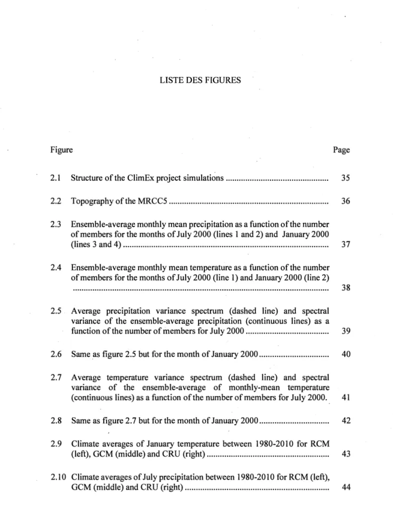
Figure 2.1 shows the structure of the simulations used in the ClimEx project, whose experimental framework is described in Leduc et al. (2019). The CanESM2 global climate model first provides 5 series of simulations with different initial conditions, which are run over a 100-year period from 1850 to 1950. Then each of these five simulations receives 10 small random disturbances to produce 50 initial conditions that progressively ~ecome independent in terms of their representation of model's internai climate variability. These random perturbations of the initial atmospheric state were introduced via a parameterization of an aspect of the cloud properties of the CanESM2 model. This approach uses a random number generator with a predefined seed. Thus,

(28)

16 the 50 individual members are based on different seeds. Consequently, different climate change realizations are produced without any changes in the physico-dynamic properties and structure of the mode 1. These CanESM2 simulations include historical forcing from 1950 to 2005 and RCP8.5 forcing from 2005 to 2100. Finally, these 50 members are used to drive the high-resolution CRCM5 model over a regional domain centred over the province of Québec. Spectral nudging of large scales (Riette and Caya 2002; Separovic et al. 2012) was applied to the horizontal components ofwind within the RCM domain. We thus obtain 50 new members (simulations) simulating the climate over Québec from 1950 to 2100 on a grid mesh of 12 km.

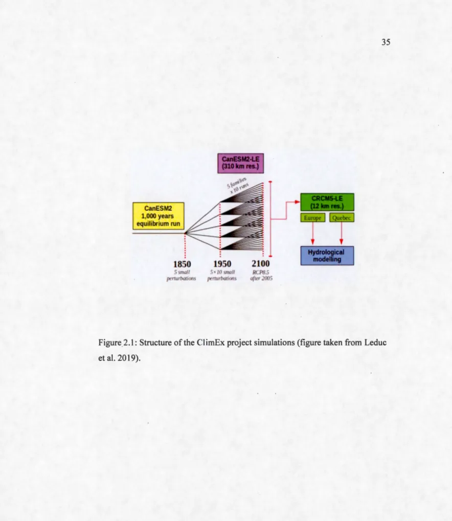
Figure 2.2 shows the regional domain used by the CRCM5, which represents the northeastem region of the American continent on a 280x280 grid point domain.

2.3.2 Choice of observation data

Severa! observational datasets were selected based on resolution, spatial coverage and temporal frequency.

CRU data:

CRU (Climate Research Unit, Time Series V3.21) data are provided by the BADC (British Atmospheric Centre). These data from measurements at weather stations around the world were gridded onto a global grid, over land only (Harris et al. 2014 ). The variables chosen are mean temperature and precipitation. They cover the period from January 1901 to December 2012 on a grid mesh of0.5°x0.5° with a monthly time interval.

GPCP data:

GPCP (Global Precipitation Climatology Project) are observational data provided by the World Climate Research Program (WCRP) on a grid mesh of 1 ° (stations and

(29)

satellites). They cover the period from 1976 to present. They have a daily temporal frequency (Huffman et al. 2009).

Daymet data:

These DA YMET (Daily Surface Weather Data) data are provided by NASA and have the highest spatial resolution, on a grid mesh of lkmx 1km. These are gridded observation analysis data on the North American continent and cover the period from 1980 to present. The temporal frequency is daily (Thornton et al. 2017)

Table 2.1 is a summary of all the data used in this project and Figure 2.2 represents the domain of analysis.

2.4 Methodology

The methodology used here to quantify the added value is composed of three successive steps: interpolation on a common grid, spatial decomposition into large and small scales and spectral analysis (or scale separation). These steps are described in sections 2.4.2 to 2.4.4. But first, the concept of added value will be defined in section 2.4.1.

2.4.1 Definition of added value

Two definitions of added value will be used in this study. The first one relates to the value of the large ensemble itself. In fact, an important motivation behind the use of large ensembles is to separate the forced climate change signal from the internai variability of the climate system (Deser et al. 2004, Deser et al. 2012a, Deser et al. 2012b, Deser et al. 2014 ). In the current study using the ClimEx dataset, it is worth noting that the term "internai variability" refers to the natural variability of the global

(30)

18 climate system (i.e. of the GCM), which is downscaled through the lateral boundary conditions of the RCM. Given that. internai variability is strongly related to the occurrence of extreme events, the first definition of added value to be used in this study will focus on the sampling of internai variability as fonction of the number of members in the ensemble. This new definition of added value extends the concept of "added variability" previously used by Bresson et al. (2009) et Di Luca et al. (2013).

The second definitfon of added value to be used in the following work is related to the high resolution of the RCM mode 1, as compared with its driving GCM and available observations with different resolutions. This concept is in line with the definitions of added value established in the work of Gleckler et al. (2008), Watterson et al. (2014)

/ and Di Luca et al. (2012), already discussed in the introduction section. To quantify this added value, these following steps (2.4.2 to 2.4.3) will be followed. The section 2.4.4 (spectral analysis) is used for both concepts (definition) of the added value.

2.4.2 Interpolation on a common grid

Comparing climate models or evaluating their performance against observational gridded data requires choosing a common resolution or grid. Thus, according to Prein et al. (2015) and Di Luca et al. (2016), two steps must be followed to compare gridded -datasets with different spatial resolutions. The first step is to choose a common grid. In this _ sense, the work of Hong and Kanamitsu et al. (2014) recommend that all comparisons should be made at the coarsest resolution among the observations, GCM and RCM. However since the goal of our study is to evaluate the added value from the different spatial scales, then the CRCM5 domain on 12km grid is chosen as common grid. This choice is natural since the GCM and analysis of observations ( except daymet data) resolution is lower than that of the RCM. This means that our study evaluates not only the added value on common spatial scales between the RCM and the GCM (large scale ), but also the added value resulting from finer scales that are not resolved on the GCM grid. Following the selection of a common grid, the next step is to choose the

(31)

interpolation method from the coarsest to the finest grid. Three classical methods are used for interpolation: nearest neighbour, bicubic and bilinear. These methods are widely used in a large number of applications because of their algorithmic simplicity and therefore their low implementation cost. A comparison of the three methods will be made below to explain the influences of each in quantifying of added value.

2.4.3 Spatial decomposition into large and small scales

RCMs have been developed to better represent climate at the regional scale compared to global models. The improved resolution of the RCMs is therefore expected to allow a better representation of atmospheric processes. Spatial decomposition is used to analyze the results in different group of scales. It also allows models to be evaluated and the relationship between meteorological phenomena of different scales to be explained (Peser et al. 2005; Feser et al. 2006; Denis et al. 2002).

In this project, the method for decomposing the spatial fields into different groups of scale is defined as follows. This is to better evaluate and quantify the added value, subsequently, from the different scales (Di Luca et al. 2016). Decomposition therefore consists in separating the atmospheric field in two or ideally in three sub-scales: large, medium and small.

• Large scales (ls): scales common to RCMs, GCMs and all observations datasets

• Medium scales (ms): scales common to RCMs and observations

• small scales (ss): scales represented only by the RCM and Daymet

There are several methods for decomposing the spatial scales. Two methods can be mentioned, for example, a spatial two-dimensional discrete filter developed by Feser et al. (2005) and a Discrete Cosine Transform (DCT) developed by Denis et al. (2002).

(32)

20 For simplicity, the DCT method is chosen in this study.

The DCT method therefore consists of separating the spatial scale by applying spectral filtering. A low-pass filter and a high-pass filter allow extracting large and small scales respectively.

Let X be our climate statistic ( e. g. a monthly average temperature ), which can therefore be broken down into large (X1_{s) and smalls (Xss) scales as follows by applying the DCT} method and according to Di Luca et al. (2013a):

X= x•s

+

xss (1)

Hence, for the RCM, the observations and the GCM respectively, the prev1ous equations can be written as:

XRcM= X1_sRCM

₊

_xssRCM ₍₂₎ Xobs=

x

1sobs

+

xssübs (3) XacM= x1_sGCM _{with xssGCM =0} ₍₄₎

2.4.4 Spectral analysis

After interpolating all the data on the RCM grid, a spectral analysis ( scale sepàration in the spectral domain) is made to compare all the data with the RCM simulations in large and small scales. To do this, the variance spectra of the simulations are calculated as a fonction of wavelength using the DCT method (Denis et al. 2002).

(33)

2.5 Results

2.5.1 Added value by the ensemble size

In section 2.4.1, the added value related to the ensemble size was discussed and defined. This added value represents the better sampling of internai variability due to the large number of members in the ensemble. A spatial approach and a spectral approach will be used to show this.

2.5.1.1 Internai variability interpreted in the spatial domain

Here, we study the sensitivity of the overall average precipitation (pr) as a fonction of the number of members (simulations). This is done here by calculating the monthly average precipitation for one member, then for two members, and so on, and up to 50 members. The 50 members or simulations of the ClimEx ensemble are named: kda, kdb, kdc up to kdz then kea, keb, kec up to kex. Figure 2.3 presents the results for the months of January and July of 2000. For simplicity, we only show the monthly average precipitation for one member, two members, three members, four members up to 7 members and then for fifty members (8 figures per month). Figure 2.3 shows that the larger the number of members for averaging precipitation, the smoother the spatial variations of precipitation, reducing the amplitude of finer scales variations. It is noted however that beyond 7 members, the spatial variability of small scales decreases quite slowly.

With regard to sensitivity by season, it can be noted that precipitation in July (summer) is slightly higher than that in January (winter), particularly over land; but the behaviour of the average as a fonction of the number of members is very similar in both seasons.

(34)

22 The same analysis is applied for air surface temperature (tas) in Figure 2.4. Unlike the case for precipitation, spatial variability is little affected by the number of members considered for the calculation of the ensemble average temperature.

In short, for precipitation, the decrease in variance is asymptotic and therefore the spatial variability decreases as n (number of members) becomes large (this discussion will be much highlighted in the next section.). This decrease in spatial variability is more important in small scales than in large scales, which highlights the fact that large-scale spatial features are fairly consistent across members in the ensemble. This can be seen in figure 2.3 as the precipitation maximum over the ocean that survives to the ensemble averaging procedure. For the small-scale features, those appear much more different across the ensemble and thus vanish after averaging over a large number of members.

With regard to temperature, this behaviour is also present, but at a smaller extent. This could be related to the fact that surface air temperature is highly affected by land surface characteristics such as soil properties, vegetation type, lake fraction, land sea contrasts or orography, which are common stationary forcings applied to all 50 members of the ensemble.

2.5 .1.2 Internai variability interpreted i~ the spectral domain

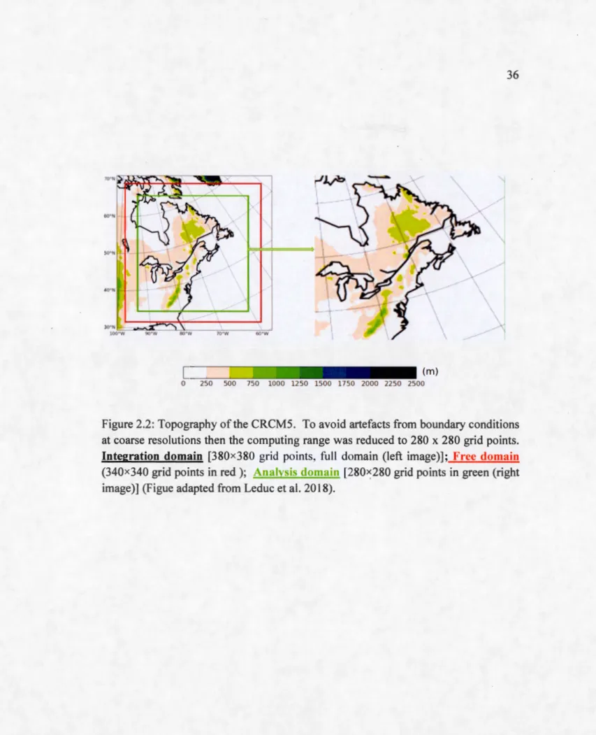
The results shown in Figures 2.3 and 2.4 has shown that the sensitivity of the ensemble mean to the number of members differs according to field and the spatial scales considered. Thus, to pursue the analysis, the DCT method is used (Discrete Cosine Transform; Denis et al, 2002). The result of a spectral decomposition using the DCT method is shown in Figure 2.5 for the monthly-mean precipitation in July 2000. The solid color curves in Figure 2.5 correspond to the spectra of the ensemble mean calculated with various number of members. In other words, to obtain these curves, precipitation variance spectra were calculated for the ensemble average of 1, 2, 3 and

(35)

so on, up to 50 members. The dotted line in Figure 2.5 corresponds to the average precipitation variance spectrum calculated from the 50 membres. This figure confirms the remark made about the results shown in Figure 2.3: the spectral variance diminishes rapidly for the the first 7 members, while beyond 7 members, the spectra converge asymptotically. Morever, it can be seen that the ensemble means of several members decrease spatial variability mainly at small scales. Figure 2.6 shows corresponding results for the month of January 2000. A detailed comparison between Figures 2.5 and 2.6 reveals that the variances decay more rapidly with increased number of members in July than in January. This can be explained by the fact that in summer, there are more fine scales than in winter.

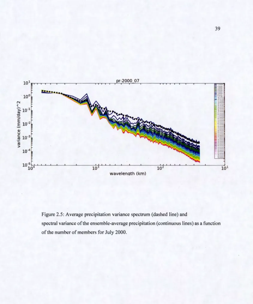
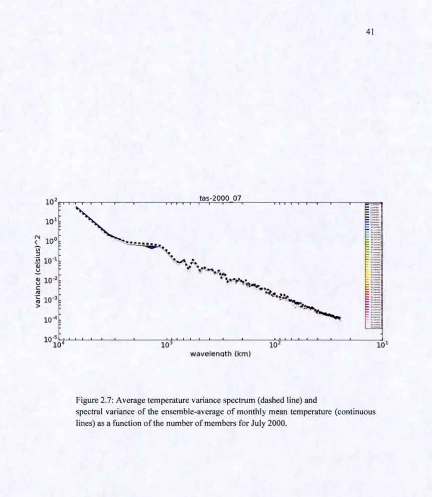
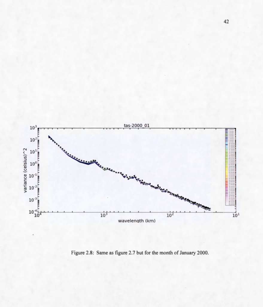
Figure~ 2.7 and 2.8 show corresponding results for temperature, in July and January, respectively. These Figures confirm the previously noted remark that ensemble-mean temperature depend little on the number of members.

It should be noted that this study is based on monthly-mean data; it should be kept in mind that different interpretation could be obtained if instantaneous or daily-mean data had been used.

2.5.2 Added value by high resolution

To quantify the added value of high resolution, the RCM will be compared with the GCM and the observation data

2.5.2.1 Overview of the climatic averages of the data on their native grid

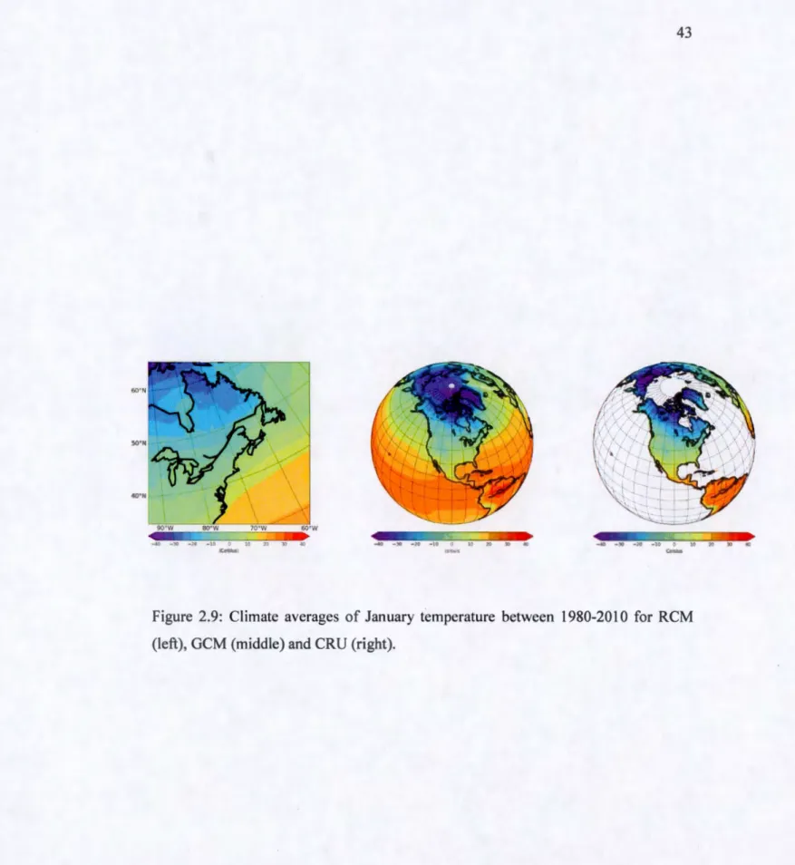
Figures 2.9 and 2.10 show the climatic averages of temperature and precipitation respectively for the months of January between the period 1980 and 2010 as obtained from the GCM, the CRU gridded observations and the RCM data on their respective native grid. The analysis in Figure 2.9 shows that the temperature variations of the three data sets are quite similar, with low temperatures in northern Québec, northern Ontario

(36)

24 and James Bay, and higher temperatures in the southem part of the regional domain, the warmest temperatures occuring in the Atlantic Ocean. However, a detailed comparison between the three datasets reveals some differences. For example, the GCM giv~s warmer temperatures over Newfoundland and Labrador compared to the RCM and CRU. lt should also be noted that, overall, the RCM temperature simulations are somewhat closer to the observations compared to those of the global GCM mode 1. The fact that the RCM better simulates climate variations in temperature here shows the added value of the RCM as compared to the GCM.

Figure 2.10 shows that the climatic averages of precipitation of the RCM, GCM and CRU are slightly different in some locations. Precipitation from CRU observations is mu.ch higher than that from the RCM and GCM in the western part of the domain. For the GCM, the highest precipitation is located on the coasts of northeastem Québec, eastem Newfoundland and Labrador and part of the Atlantic Ocean. Similarly, the highest precipitation for RCM is located in these same areas. Also, spatial variability of small scales, certainly reduced because of the climate average, are noted in the RCM simulations. However, to have a more rigorous comparison and thus better quantify the added value, an interpolation on a common grid is necessary.

2.5.2.2 Data comparison after interpolation on the RCM grid

Figure 2.11 shows the summerprecipitation averages (2010) of the GCM, CRU, GPCP data interpolated on the RCM grid using the linear, cubic and nearest neighbour methods, and of the RCM (see figure for more description). No matter the interpolation method used, fine-scale spatial variability is only present in the RCM fields, and these are more localized in coast, ocean and Great Lakes. This presence of spatial variability in small scales reflects the potential existence of added value of the RCM. The high-resolution RCM therefore allows simulating small scale structures.

(37)

Moreover, a comparison between the three methods show that the linear and cubic methods are very similar, but quite different from the nearest neighbour method. It can also be noted that the nearest neighbour interpolation makes it easier to highlight the structure of small scales compared to the other two methods. The nearest neighbour method is therefore the best interpolation for qualitatively describing the added value of the regional model when comparing with maps from others datasets.

A detailed comparison of precipitation variations between all these data shows that the GPCP and CRU analyses of observations are fairly closer. For these observational data, the average precipitation varies between 2 and 12 mm/day. The maximum values are located over the ocean. RCM precipitation is lower on the continent but significant over the ocean. The RCM simulations are more closely related to the observations (CRU and GPCP) compared to the GCM simulations.

2.5.2.3 Data comparison after separating large- and small-scale features

It has been shown prevfously that the spatial decomposition or filtering of large and small scales makes it possible to better quantify the added value from the spatial scales considered. To show this, we filter large and small scales using the DCT (Discrete Cosine Transform) method. In order to separate the spatial fields into these two groups of scales, a cut-off wavelength of 640 km was defined, which correspond to the smallest wavelength (i.e twice the nominal grid resolution) provided by the GCM as lateral boundary conditions for driving the RCM. Figure 2.12 shows the large and small -scale components of the monthly-mean precipitation of the RCM, GCM and GPCP ( a single member is used here ). The RCM precipitation exhibits substantial fine scales near the Laurentian mountains, over the ocean and at the coastline where surface forcings are better resolved in high-resolution models. The GPCP also shows some small scales in the ocean, as the separation wavelength ( defined for the GCM) was larger than twice the nominal resolution of this dataset. By construction of the DCT filter, the decomposition of the GCM fields should not give any fine scales since the

(38)

26 separation wavelength corresponds exactly to the nominal resolution of this dataset; as expected, DCT low-pass filtering shows hardly any fine-scale spatial variability of precipitation over mountains and coastal regions. The decomposition into large and small scales shows here that atmospheric process structures and surface contrasts are better represented in the high-resolution regional mode 1. Hence the added value of the RCM compared to the GCM.

2.5 .2.4 Spectral analysis

Spectral decomposition allows to compare RCM simulations with those of the GCM and observation data for any spatial scale. Aft~r interpolating all data on the regional model grid and then applying the DCT method, the variance spectrum of July mean precipitation is calculated for the RCM, GCM and GPCP. Figure 2.13 presents the precipitation variance spectra of the 50 individual members for July 2010 for the RCM and the GCM. The vertical dotted lines correspond to the eut-off wavelengths of the GCM and GPCP: the longest eut-off wavelength is twice the grid mesh of the GCM (640 km, in red) and the shortest is twice the grid mesh of the GPCP (200km, in black). As a generalization of the previous separation into small and large scales (see equations (1) to (4)), these cut-offwavelengths allow here to <livide the spectral domain into three distinct groups of scales:

1)

the large scales resolved in all datasets, 2) the medium scales resolved by GPCP and the RCM, and 3) the small scales only resolved by the RCM. Figure 2.13 shows that the variance spectra of the RCM and GCM members are very similar to the GPCP in the large scales, i.e. wavelengths greater than 640 km. On the other hand, for wavelengths between 640 and 200km, i. e. the medium scales, the spectra of the RCM and GCM differ irtcreasingly when approaching the short wavelengths. The variance spectra of the GCM decreases rapidly beyond its eut-off wavelength and thus by construction does not present information in medium and small scales. Both the RCM and GPCP spectra decrease slightly and at a similar rate in the medium scales, althought the GPCP variance is much smaller. For the small scales,

(39)

which are not represented in the GCM and GPCP, the RCM's added value cannot be evaluated. Similarly, it is not clear whether GPCP is correctly representing variability in the medium scales, since its variance is significantly smaller than the RCM in this spectral window. In addition, we also note that the variance spectra of the RCM individual members overlap in all large, medium and small scales. This means that the individual members of the RCM have almost the same variances at different spatial scales. The variance spectra of the GCM and GPCP are quite negligible in small scales. The resolution of the GPCP observation data (1 °) is therefore too coarse to be used to validate the spatial variability of the small scales of the RCM. To solve this problem, then observation data with higher resolutions, such as CRU data at 50 km and Daymet data at 1 km, will be used to compare with the RCM in small scales. However CRU and Daymet data do not cover the oceans and Daymet data are known to show some inconsistent values in central Québec where a limited number of meteorological stations are available; therefore, a sub-domain will be used to make the comparison with the RCM; the sub- domain chosen is the Great Lakes region

2.5.2.5 Spectral analysis in the Great Lakes sub-domain

The selected subdomain covers Lakes Superior, Michigan, Huron, Erie and part of Lake Ontario, as shown in Figure 2.14. The spectral decomposition is calculated as before, but over a smaller domain, thus allowing to compare simulations with the higher-resolution gridded observation CRU and Daymet. Figure 2.15 presents the spectral variance ofmontly inean July precipitation for the years 1998 to 2012, for the RCM, CRU, GCM, Daymet; the various curves represent individual years. The RCM simulations driven by reanalyses (RCM _ ERA) are also added. The vertical dotted lines correspond to the eut-off wavelengths of the GCM and CRU; the longest eut-off wavelength is twice the resolution of the GCM (640 km, in red) and the shortest is twice the resolution of the CRU (100km, in yellow). Figure 2.15 shows that the spectra of the RCM driven by the global model (GCM) and the RCM driven by reanalyses

(40)

28

(RCM_ERA) are almost identical in large and small scales except that the spread between the spectra appears smaller for the RCM _ ERA run. At large scales, all data exhibit similar variance spectra; but at small scales, significant differences are noted. The small-scale variance of the GCM is negligible, as is that of the CRU data. The Daymet spectrum presents information at wavelengths shorter than 640 km, i.e. fine-scale spatial variability. The RCM also shows spatial variability in small fine-scales. At small scales the behaviours of the RCM and Daymet observational data are very similar compared to the GCM. This shows the existence of the added value of the RCM compared to the GCM.

2.6 Discussion and conclusions

The goal of the project was to quantify the added value of the Canadian CRCM5 high-resolution regional model simulations compared to those of the global CanESM2 model.

In section 2, we described the simulations of the ClimEx ensemble from the CRCM5 and the CanESM2 model data. W e also explained the choice of observational datasets. In the methodology section, we started by defining two added value concepts that are adapt~d to the context of the project. The first was defined for the quantification of value added by the size of the large ensemble of the CRCM5. An_d the second concept was related to the added value of the high resolution of the regional model. Then we discussed the different other · parts of the methodology. We .have shown that interpolation on a common grid, filtering oflarge and small scales and spectral analysis are tools for detailed quantification for the second concept of added value.

In the first part of the results, we quantified the added value of the size of the ensemble using a spatial and spectral approaches. W e have shown that this allows a better sampling of internai variability. This step bas made the following statements:

(41)

• The ensemble averaging of several members decreases spatial variability (mainly in small scales for precipitation) but little for temperature.

• The sensitivity of the overall mean ofprecipitation depends on the spatial scales considered

In the second part of the results, we also quantified the added value of the high resolution of the CRCM5 by comparing it with CanESM2 and the observational datasets. To do this, we used different interpolation methods. We concluded that the cubic and linear methods were very similar while different from the nearest neighbour method. W e have shown that the nearest neighbour method is the best interpolation method for a qualitative comparison between datasets with different resolution. Interpolation has also made it possible to better highlight the spatial variability of precipitation in the small scales that are only represented in the CRCM5. This reflects the added value of the CRCM5 compared to CanESM2. W e have also discussed, the filtering of large and small scales. This spatial decomposition made it possible to highlight the structure of the fine scales of the CRCM5 and the impossibility of CanESM2 to reproduce the spatial variability of precipitation. The last step of the . results was devoted to spectral analysis. This step compared the CRCM5 with CanESM2 and observational data at large and small scales. This spectral analysis ( or scale separation) showed that the simulations of the CRCM5 were very similar to those of CanESM2 and the observation data in the large scales. The difference observed between the data was at the small scale level. The choice of very high resolution Daymet data validated the spatial variance of the small scales.

In short, we can say here that our methodology has produced satisfactory results. W e were able to show the added value of the CRCM5. Comparison of all data showed that the CRCM5 simulations were much closer to the observations compared to those of CanESM2. W e also noted that the added value was much higher at the coastal and mountain level. This can be explained by the fact that these regions experience surface

(42)

30 contrasts that are better represented in a high-resolution regional model. We also found that the value added was much more evident in short periods of time, for example monthly averages.

Furthermore, we have shown the ergodic character of the members of the large ensemble (see appendix for demonstration). Which allows to know the statistics of a member from a single achievement.

However, there are some drawbacks to this project. The resolution of GPCP observation data is too low to be able to compare and validate fine-scale structures throughout the field of study. The Daymet data, despite their high resolution (1 km), are not covering the oceans and sometimes have erroneous values in central Québec. The Great Lakes sub-domain chosen here is too small for a more rigorous comparison.

It would be interesting for future studies to find high-resolution observational data that have land-ocean coverage.

A more detailed quantification of the added value for extreme events would also be interesting to study.

We want to mention that this study is based on monthly-mean data; it should be kept in mind that different interpretation could be obtained if instantaneous or daily-mean data had been used.

(43)

Acknowledginents

The ClimEx project was funded by the Bavarian State Ministry for the Environment and Consumer Protection. The CRCM5 is developed by the ESCER Centre of the Université du Québec à Montréal (UQAM; www.escer. uqam.ca) in collaboration with Environment and Climate Change Canada. W e acknowledge Environment and Climate Change Canada's Canadian Centre for Climate Modelling and Analysis for executing and making available the CanESM2 Large Ensemble simulations used in this study, and the Canadian Sea Ice and Snow Evolution Network for proposing the simulations. Computations with the CRCM5 for the ClimEx project were made on the SuperMUC supercomputer at Leibniz Supercomputing Centre (LRZ) of the Bavarian Academy of Sciences and Humanities. The operation of this supercomputer is funded via the Gauss Centre for Supercomputing by the German Federal Ministry of Education and Research and the Bavarian State Ministry of Education, Science and the Arts.

We would like to thank the Centre ESCER (Étude de la Simulation du climat à l'Échelle Régional) of UQAM, the consortium of Ouranos and the MIT ACS pro gram for their financial support.

(44)

(45)

2.1 Structure of the ClimEx project simulations 2.2 Topography of the CRCMS

2.3 Ensemble-average monthly mean precipitation as a fonction of the number ofmembers for the months of July 2000 (lines 1 and 2) and January 2000 (line.3 and 4)

2.4 Ensemble-average monthly mean temperature as a fonction of the number ofmembers for the months of July 2000 (line. l) and January 2000 (line 2) 2.5 Average precipitation variance spectrum ( dashed line) and spectral variance of the ensemble-average precipitation (continuous lines) as a fonction of the number of members for July 2000

2.6 Same as figure 2.5 but for the month of January 2000

2. 7 Average temperature variance spectrum ( dashed line) and spectral variance of the ensemble-average of inonthly-mean temperature ( continuous lines) as a fonction of the number of members for July 2000 2.8 Same as figure 2. 7 but for the month of January 2000

2.9 Climate averages of January temperature between 1980-2010 for RCM (left), GCM (middle) and CRU (right)

2.10 Climate averages of July precipitation between 1980-2010 for RCM (left), GCM (middle) and CRU (right)

(46)

2.11 Summer mean precipitation interpolated on the RCM grid with linear methods (linel). Cubic (line2) and nearest neighbour (line3)

2.12 Large and small scale decomposition of precipitation for July 200l for the RCM (line 1 ), GCM (line 2) and GPCP (line 3)

2.13 Spectral variance of the precipitation of the 50 individual members for the month of July 2010 for the RCM (blue) and for the GCM (red). The black curve represents the variance spectrum of the July 2010 precipitation for the GPCP

2.14 Analysis sub-domain centred over the Great Lakes

34

2.15 Spectral variance of montly mean precipitation from July for the years 1998 to 2012 for the RCM, CRU, GCM, Daymet and RCM_ERA

(47)

canESM2

000 years equilibrium run

1950 2100

µ

Figure 2.1: Structure of the ClimEx project simulations (figure taken from Leduc et al. 2019).

(48)

36

(m)

0 250 500 750 1000 1250 1500 1750 2000 2250 2500

Figure 2.2: Topography of the CRCM5. To avoid artefacts from boundary conditions at coarse resolutions then the computing range was reduced to 280 x 280 grid points.

Integration domain [380 x380 grid points, full domain (left image)]; Free domain

(340 x340 grid points in red ); Analysis domain [280~280 grid points in green (right

(49)

SO'N 40'N 60"N SO"N 40•N 60"N 50'N 40' N 60'N SO'N 40•N SO'N 40 •N 60'N 50'N 40' N 60'N 50'N 40' N 60'N SO'N 40' N 4 6 1 10 12 1' mmldty 4 0 1 10 mmldty 50'N 40'N 60' N 50'N <IO' N 60'N SO' N 40• N 60'N 50'N 40' N è Ci 1 10 mmtdty

Figure 2.3: Ensemble-average monthly mean precipitation as a fonction of the number of members for the months of July 2000 (lines 1 and 2) and January 2000 (lines 3 and

(50)

- - --60"N 40• N - 12 -6 O 6 12 11 2-4 30 '6 Celsius 50"N 40•N 40' N 60"N 40' N 90 'W -JO - 2• - li -12 -6 0 - JO -24 -li -12 -6 0 0

Celsius Celsius Celsius

60"N 60"N

SO'N

40"N 40"N

Figure 2.4: Ensemble-average monthly mean temperature as a fonction of the number of members for the months of July 2000 (lines 1 and 2) and January 2000 (lines 3 and

(51)