Pablo Arbel´aez ([email protected]) and Laurent D. Cohen ([email protected])
CEREMADE, UMR CNRS 7534 Universit´e Paris Dauphine,
Place du mar´echal de Lattre de Tassigny, 75775 Paris cedex 16, France
Abstract. We address the issue of low-level segmentation of vector-valued images, focusing on the case of color natural images. The proposed approach relies on the formulation of the problem in the metric framework, as a Voronoi tessellation of the image domain. In this context, a segmentation is determined by a distance transform and a set of sites. Our method consists in dividing the segmentation task in two successive sub-tasks : pre-segmentation and hierarchical representation. We design specific distances for both sub-problems by considering low-level image attributes and, particularly, color and lightness information. Then, the interpretation of the metric formalism in terms of boundaries allows the definition of a soft contour map that has the property of producing a set of closed curves for any threshold. Finally, we evaluate the quality of our results with respect to ground-truth segmentation data.
To appear in International Journal of Computer Vision, Special issue on Variational and Level Set methods
Keywords: image segmentation, distance transforms, path variation, ultrametrics, vector-valued image, color, boundary detection.
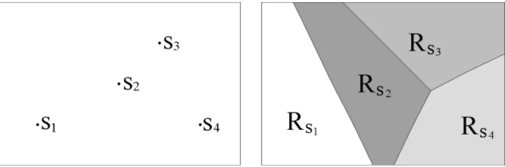
Figure 1. Set of sites and Euclidian Voronoi tessellation.
1. Introduction
The metric framework for spatial tessellations was first formalized by Dirichlet (Dirichlet, 1850) and Voronoi (Voronoi, 1907), who studied the idea of partition-ing the space by considerpartition-ing a finite set of fixed points, called sites, and assignpartition-ing each point to the closest site. The regions defined by this construction are usually called Voronoi regions or Voronoi cells and the resulting spatial decomposition is known as a Voronoi tessellation or Voronoi diagram. Figure 1 presents an example of this structure in its original formulation: a rectangle in the plane is partitioned by measuring the Euclidian distance between each point and the four sites shown on the left. In this case, the Voronoi regions are convex polygons.
Since its early introduction, the Voronoi tessellation has found application in a wide range of disciplines and has inspired several generalizations (Aurenhammer and Klein, 2000; Okabe et al., 2002). In the context of image analysis, application of this structure includes compression (Ahuja et al., 1985), texture classification (Tuceryan and Jain, 1990) and shape representation (Mayya and Rajan, 1996). In this paper, we consider an extension of the Voronoi tessellation to pseudo-metric spaces and we study its application to the segmentation of vector-valued images, focusing on color images. Within this framework, segments are defined as Voronoi regions of a set of sites, relatively to a pseudo-metric. The problem is thus transferred to the definition of a relevant distance transform from the image data and the selection of a set of sites. Our approach consists in applying the
metric formalism to two successive sub-tasks of segmentation : pre-segmentation and hierarchical representation of color images. For this purpose, we design specific distances by considering two low-level image attributes, namely color and brightness information.
We first present a pre-segmentation technique called the extrema mosaic. The pseudo-metric defined in this part, the path variation, is a generalization of the one dimensional total variation for vector-valued functions of multiple variables. In the case of color images, we study the Voronoi tessellation obtained by considering the extrema of the lightness channel of the image as sites. This method provides a natural reconstruction of the image that offers a balance between content conservation and simplification.
In the second part, we focus only on those tessellations that are invariant when a site is displaced inside its Voronoi region. This consideration leads to a type of pseudo-metrics called the ultrametrics. These distances are useful for a multiscale representation of the image, as their definition amounts to construct-ing a stratified hierarchy of partitions of the image domain. Startconstruct-ing from the pre-segmented image, we define an ultrametric for color image segmentation. This distance incorporates boundary and inner region information.
Finally, we exploit the boundary-based formulation of the metric formalism to define a soft boundary image, which we call ultrametric contour map (UCM). Our approach guarantees that a threshold in this image supplies a set of closed curves. The UCM is then used to evaluate the quality of our results with respect to ground-truth human segmentations.
This paper is organized as follows. Section 2 presents the mathematical frame-work. Section 3 introduces our pre-segmentation method. Section 4 is dedi-cated to hierarchical segmentation and ultrametric contour maps. Finally, the evaluation of our results is discussed in Section 5.
2. Voronoi Tessellations
In this section, the classic notion of Voronoi tessellation is extended to the framework of pseudo-metric spaces.
Definition 1. A pseudo-metric space (Kelley, 1975; Kuratowski, 1966) is a
pair (Ω, ψ) where Ω is a set and the application ψ : Ω2 → IR+ satisfies the
following axioms:
1. ψ(x, x) = 0, ∀x ∈ Ω .
2. ψ(x, y) = ψ(y, x), ∀x, y ∈ Ω.
3. ψ(x, y) ≤ ψ(z, x) + ψ(z, y), ∀x, y, z ∈ Ω.
The number ψ(x, y) is called the distance between x and y.
A pseudo-metric space is convex if each pair of points x, y ∈ Ω can be joined by a ψ-straight path, i.e., a continuous application γ : [a, b] → Ω such that :
∀ t ∈ [a, b], ψ(x, y) = ψ(x, γ(t)) + ψ(γ(t), y).
Definition 2. Let (Ω, ψ) be a closed convex pseudo-metric space and S = {s1, ..., sn} ⊆ Ω a set of fixed points called sites.
The Voronoi region, or V-region, of a site si ∈ S is defined as: Rsi = {x ∈ Ω| ψ(x, si) ≤ ψ(x, sj), ∀j ∈ {1, ...n}, j 6= i}.
The Voronoi tessellation, or V-tessellation, of Ω associated with ψ and
S is the set of Voronoi regions: Π(ψ, S) = {Rs1, ..., Rsn}.
Note that Axiom 1 of Definition 1 allows different points to be at zero distance in a pseudo-metric space. By considering the equivalence classes ˆx(ψ) = { y ∈
Ω | ψ(x, y) = 0}, one can define a quotient space bΩ(ψ) which is a metric space. Each element of a V-tessellation is therefore a union of elements in bΩ(ψ). The
equivalence classes indicate the level of resolution of the pseudo-metric, under which the distance is blind.
Two main differences between our approach and the standard framework of Voronoi tessellations (Aurenhammer and Klein, 2000; Okabe et al., 2002) are worth noting. First, by considering pseudo-metrics we have access to a class of spaces larger than the metric spaces. Second, since we aim at applying this structure to image analysis, the set Ω corresponds to the domain of definition of a color image and the pseudo-metrics we study depend explicitly on the image data.
Hence, in this context, the segmentation of a color image is determined by the definition of a relevant pseudo-metric and the selection of a set of sites; the rest of the paper is dedicated to these issues. However, as we make no assumption on the image content, we only consider as set of possible contours the discontinuities of the original image. This property can be obtained by defining the pseudo-metric
ψ such that the equivalence class of a point x ∈ Ω coincides with the connected
component of u that contains x. The quotient space bΩ(ψ) is then homeomorphic to the space of components of the image. Moreover, for a set of sites S, each element of Π(ψ, S) is a union of components of u. Such V-tessellations simplify then the image while preserving its original contour information.
Finally, in order to address the segmentation of color images in the metric framework, a practical problem is the definition of a distance between colors. For this issue, the C.I.E. standard L∗ab (Wyszecki and Stiles, 1982) is adopted
in this paper. This color representation ought to approximate a perceptually uniform color space. Though not perfect, it provides two main advantages with respect to the basic RGB system: first, the separation of the color information into a lightness channel L∗ and two chromatic channels a∗ and b∗; second, the
approximation of the metric in the Riemannian color space by the Euclidian distance. In the sequel, the distance in the color space L∗ab is noted by δ∗.
3. Pre-segmentation
This section presents an application of the metric formalism to the pre-segmentation of color images. For this purpose, we begin by defining a specific distance.
Let (X, ψ) be a pseudo-metric space. Consider a finite partition of an interval [a, b], σ = {t0, ..., tn}, such that a = t0 < t1 < ... < tn = b and denote by Φ the
set of such partitions.
The variation at order p of a function f : [a, b] → (X, ψ), is given by :
vp(f ) = sup σ∈Φ n X i=1 ψp(f (t i), f (ti−1)).
If (X, ψ) is the set of real numbers with the usual metric, then v1(f ) corresponds
to the total variation of f , the well known functional introduced by Jordan (Jordan, 1881). In our case, (X, ψ) will be the color space (L∗ab, δ∗).
For multiple variable functions, we measure the minimal variation on all the paths between two points:
The path variation at order p of a function u : Ω → (X, ψ), is defined as:
Vp
u(x, y) = inf γ∈Γxy
vp(u ◦ γ), ∀ x, y ∈ Ω. (1)
where γ is a continuous path between x and y and Γxy the set of such paths.
Note that, in contrast to the usual notion of total variation for functions of multiple variables (Rudin et al., 1992), the path variation is defined at each point of Ω. By definition, the equivalence class bx(Vp
u) coincides with the connected
component of u containing x. A discrete definition of this distance for color images can be found in (Arbel´aez and Cohen, 2003a).
The path variation is an interesting pseudo-metric for a local level of analysis, as it quantifies the minimal variation of color between pixels. In order to apply this distance to pre-segmentation, we now turn to the selection of an appropriate set of sites.
The purpose of pre-segmentation is to decompose the image into local entities that preserve its geometric structure. Therefore, the spatial distribution of sites
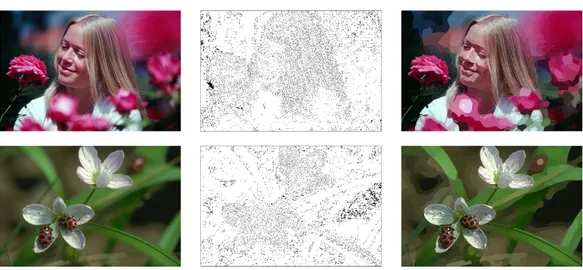
Figure 2. Form left to right: Original images, sites and extrema mosaics.
should be physically representative of the image content and each significative feature should contain at least one of them. In the case of natural images, the lightness extrema satisfy these two properties, as shown in Figure 2.
Thus, we consider the Voronoi tessellation Π(Vp
u, ext(u)), where ext(u)
de-notes the set of extremal components of the lightness channel L∗ of a color
image u. An extrema mosaic of u is a piecewise constant reconstruction of the image, obtained by assigning a color to each V-region of Π(Vp
u, ext(u)).
Figure 2 illustrates the method. The central column presents the sites in black and the extrema mosaics are shown on the right, with the V-regions depicted on their mean color. The density of the lightness extrema is high on focused or textured regions and low in blurred or homogeneous zones. Consequently, the blur is reduced in the reconstructed images, while the geometric structure, including notably contour information, is preserved.
Hence, the choice of the path variation as the pseudo-metric and the spatial distribution of the sites determine a V-tessellation where a balance between simplification and content conservation is obtained. In the sequel, the extrema mosaic is used as a parameter-free pre-segmentation method. This approach may also be combined with a non-linear diffusion filtering in order to reduce
the number of extrema and regularize the tessellations (Arbel´aez and Cohen, 2003b).
4. Hierarchical Segmentation
In the framework of Voronoi tessellations, segments are modelled as Voronoi regions. It is then desirable that displacing the site inside a V-region does not modify its boundary. Unfortunately, the path variation does not satisfy this property. The rest of this paper is dedicated to the study of a particular type of pseudo-metrics exhibiting this invariance requirement.
4.1. Stratified Hierarchies and Ultrametrics
Ultrametrics are a standard tool in data analysis (Benz´ecri, 1984). They are often used for clustering because they determine a particular type of strong hierarchies. These distances are thus naturally suited for a multiscale representation of the image.
A stratified hierarchy is a family of nested partitions H together with a function st : H → IR, called a stratification index, such that: ∀ a, b ∈ H : a ⊂
b ⇒ st(a) < st(b).
An ultrametric space (Ω, ψ) is a pseudo-metric space for which Axiom 3 of Def. 1 is replaced by the stronger relation: ψ(x, y) ≤ max{ψ(z, x), ψ(z, y))}.
The topology induced by an ultrametric differs significantly from the usual Euclidian case. In particular, two ultrametric balls can only be disjoint or nested. Consequently, the set of all the closed balls for a fixed radius r determines a Voronoi tessellation, noted Π(ψ, r). The family H = {Π(ψ, r)}r≥0is then a family
of nested partitions of Ω. A stratification index for H is given by the function that assigns to each ultrametric ball its radius. Conversely, each stratified hierarchy defines an ultrametric distance.
If a Voronoi tessellation is determined by an ultrametric, the previous prop-erties imply that replacing a site si ∈ S by another point s0i in the interior of
its Voronoi region Rsi does not modify the V-tessellation. These pseudo-metrics
satisfy then the invariance requirement mentioned at the beginning of the section. Moreover, the problem of selecting a set of sites can be addressed in this case through the choice of a radius r for the ultrametric V-regions. In the sequel, the ultrametrics are normalized in order to assign the value of 1 to the radius of the smallest V-region that contains the whole domain.
4.2. An ultrametric for Segmentation
In this subsection, we define a specific ultrametric for the segmentation of color images. Its construction is derived from the characterization of this type of distances as stratified hierarchies.
A family of nested partitions can be constructed by a graph based region merging strategy. Such a clustering approach consists in progressively merging regions of an initial partition according to a dissimilarity measure, a real valued function defined for each pair of adjacent subsets of the domain (Garrido et al., 1998; Forsyth and Ponce, 2003).
However, in order to define a stratified hierarchy H, the dissimilarity d must be compatible with the hierarchical order:
a ⊂ a0∧ b ⊂ b0 ⇒ d(a, b) < d(a0, b0), ∀ a, a0, b, b0 ∈ H. (2)
In our case the ultrametric is constructed in two steps. First, we use the color information to quantify the contrast between V-regions. For this purpose, a contrast dissimilarity, noted dc, is defined as:
dc(R 1, R2) = P δ∗(p 1, p2) length(∂(R1, R2))
where δ∗ is the color distance and the sum is calculated on all the adjacent pixels
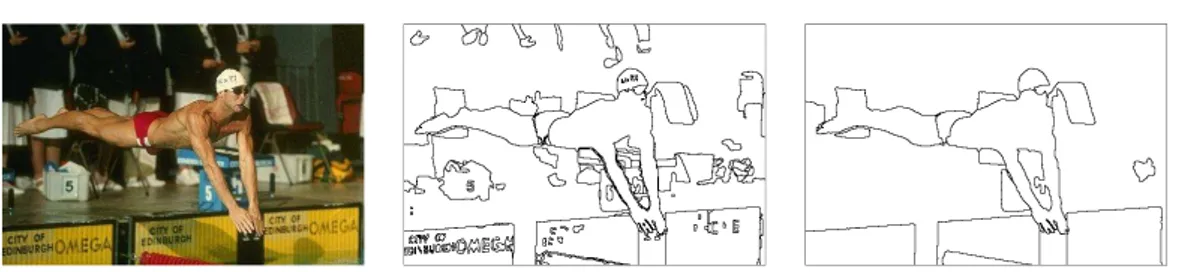
Figure 3. From left to right : Original image, tessellations Π(Υ0, 0.35) and Π(Υ0.2, 0.35).
measures the average color difference in the common boundary of the regions, on the extrema mosaic. Note that dc satisfies Equation (2).
In order to complement the boundary information supplied by dc, we measure
an internal attribute, a positive real valued function A, in each V-region. The attribute is required to be increasing with the inclusion order. Thus, starting from dc, a new dissimilarity dα is defined by the formula:
dα(R
1, R2) = dc(R1, R2) · min{A(R1), A(R2)}α.
Since A is increasing and dc is compatible with the hierarchical order, so is dα. The associated ultrametric, noted Υα, incorporates boundary as well as
internal information of the V-regions. For the examples presented in this paper, the attribute is the size of the V-region. The parameter α ≥ 0 weights the balance between contrast and area. Note that, as for the path variation, the equivalence class of a point x, ˆx(Υα), coincides with the component of the image
that contains x. Thus, the quotient space bΩ(Υα) is also homeomorphic to the
space of components of the image.
Figure 3 illustrates the influence of α in the ultrametric. The central and right images show the V-tessellations associated to the same normalized radius
r = 0.35, for the ultrametrics Υ0 and Υ0.2 respectively. Since the first distance is
determined only by the contrast, small and contrasted regions, as the letters, are extracted. When α = 0.2, these regions are eliminated from the V-tessellation. Thus, the choice of α allows the ultrametric to adapt to the image content or a particular application.
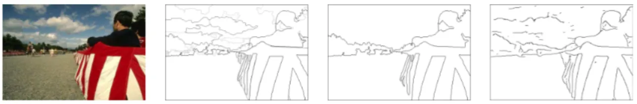
Figure 4. From left to right : Original image, UCM, thresholded UCM and thresholded local
edge detector.
4.3. Ultrametric Contour Map
Many segmentation approaches provide only binary boundary maps, while soft edge maps generated by local edge detectors often require contour completion techniques in order to obtain closed curves. The formulation of the segmentation problem in the metric framework and the use of ultrametric distances provide a natural way to fill this gap. For this purpose, the following notion is central.
The saliency of a point x in an ultrametric space (Ω, Υ) is defined as the highest radius λ such that x belongs to a boundary of the V-tessellation Π(Υ, λ). The valuation of each point by its saliency determines a real-valued image, called in the sequel a ultrametric contour map (UCM). This single image is a compact representation of the ultrametric space: a threshold in the UCM supplies the set of boundaries of the corresponding V-tessellation. This idea was first used in (Najman and Schmitt, 1996) to valuate the watershed arcs of a gradient image. The interest of this soft boundary map is that it combines the strong points of both region-based segmentation methods and edge detectors. On one hand, the value at each point is given by the hierarchical structure and is therefore not restricted to the information of a local neighborhood. On the other hand, a threshold of an ultrametric contour map provides by definition a set of closed curves. Figure 4 shows an example of UCM, with dark intensities representing high saliency. For comparison, the right image presents the optimal threshold of a state of the art local edge detector (Martin et al., 2004).
5. Evaluation of Results
In order to measure the quality of our results, we used as ground-truth the Berkeley Segmentation Dataset and Benchmark (BSDB), a database of images representing natural scenes, manually segmented by humans (Martin et al., 2001).
A methodology for evaluating the performance of boundary detectors with this database was developed in (Martin et al., 2004). It is based on the comparison of detected edge points with respect to human boundaries using the precision-recall framework (van Rijsbergen, 1979). Precisely, two quality measures are considered, precision (P), defined as the fraction of real boundaries among de-tected boundaries and recall (R), given by the fraction of detections among real boundaries. Measuring these quantities for different thresholds of the detector provides a parametric precision-recall curve. The two quantities can be combined in a single descriptor, the F-measure, defined as the harmonic mean of precision and recall: F (P, R) = 2P R/(P + R). The maximal F-measure is then used as a summary statistics for the quality of the detector on a given set of images.
Our system has a number of free parameters, intended to allow its adaptation to a particular application or type of images. In the pre-segmentation stage, these are the order of the path variation, the model to represent the V-regions and the number of iterations of the extrema mosaic. The hierarchical representations defined in Section 4 depend also on the parameter α. Additionally, we consider a weighting factor between the chrominance and the lightness in the color space. Using the ultrametric contour maps, all these free parameters were optimized with respect to the set of 200 train images of the BSDB. The optimal threshold of the UCM provided then the best radius λ for the ultrametric V-tessellations Π(Υα, λ). The set of optimal parameters was then used to benchmark our method
on the independent test set of 100 images of the BSDB. Figure 5 shows some results. The right column presents the thresholded UCM superimposed on the
(a) (b) (c) (d) (e) Figure 5. a: original images. b: human segmentations. c: UCM. d: thresholded UCM. e: (d)
superimposed on (b).
human segmentations. True positives are depicted in thick black, false positives in thick blue and missed detections in yellow.
The precision-recall methodology permitted also the comparison of our results with the Berkeley Segmentation Engine (BSE). In this approach (Fowlkes et al., 2003), region and boundary features are used to design an affinity function between pairs of pixels. The cues are optimized with respect to the BSDB and then combined with a classifier trained on the ground-truth data.
(a) (b) (c) (d) Figure 6. a: original images. b: human segmentations. c: BSE. d: thresholded UCM.
In order to make the comparison between the two algorithms fair, we used the thresholded UCM instead of the richer soft boundary map. We obtained
F (0.62, 0.64) = 0.63 for our method and F (0.61, 0.65) = 0.63 for the BSE.
Thus, the overall precision is higher for the UCM, while the BSE provides better overall recall. The probability that the detector’s signal is valid is then higher with our system while the probability that the ground-truth data was detected is higher with the BSE. However, the two descriptors are very close and the overall F-measures are equivalent.
Qualitatively, the results of the two methods show bigger differences, as pre-sented in Figure 6. On one hand, since the BSE is biased towards convex
seg-ments, regions with intricate boundaries are better extracted with the UCM. On the other hand, as the ultrametric Υα does not use texture information explicitly,
the BSE results are better on textured images. Both methods show nevertheless poor performances when prior knowledge about the image content is determinant for human segmentation.
Finally, the overall F-measure for the human segmentations, when compared among them, is F (0.90, 0.70) = 0.79 on the test set. This score quantifies the human performance for this task and serves as the ultimate goal for machine segmentation. The gap between the two tested methods and human performance is mainly due to precision (almost 0.3) while recall difference is only about 0.05. Thus, the efforts should be put on diminishing the noise in the segmentation algorithms. In our case, future work includes the definition of pseudo-metrics for which the information about the texture and the regularity of the contours are also taken into consideration.
References
Ahuja, N., B. An, and B. Schachter: 1985, ‘Image Representation Using Voronoi Tessellation’.
CVGIP 29(3), 286–295.
Arbel´aez, P. A. and L. D. Cohen: 2003a, ‘Generalized Voronoi Tessellations for Vector-Valued Image Segmentation’. In: Proc. 2nd IEEE Workshop on Variational, Geometric and Level
Set Methods in Computer Vision (VLSM’03). Nice, France.
Arbel´aez, P. A. and L. D. Cohen: 2003b, ‘Path Variation and Image Segmentation’. In: Proc.
4th International Workshop on Energy Minimization Methods in Computer Vision and Pattern Recognition (EMMCVPR’03). Lisbon, Portugal, pp. 246–260.
Aurenhammer, F. and R. Klein: 2000, Handbook of Computational Geometry, Chapt. 5: Voronoi Diagrams, pp. 201–290. Elsevier Science Publishing.
Benz´ecri, J. P.: 1984, L’Analyse des Donn´ees. Tome I: La Taxinomie. Paris: Dunod, 4 edition. Dirichlet, P. G. L.: 1850, ‘Uber die Reduction der positiven quadratischen Formen mit drei
Forsyth, D. A. and J. Ponce: 2003, Computer Vision: A Modern Approach. Prentice Hall. Fowlkes, C., D. Martin, and J. Malik: 2003, ‘Learning Affinity Functions for Image
Segmenta-tion: Combining Patch-based and Gradient-based Approaches’. In: Proc. CVPR. Madison, WI, USA, pp. 54–61.
Garrido, L., P. Salembier, and D. Garcia: 1998, ‘Extensive Operators in Partition Lattices for Image Sequence Analysis’. IEEE Trans. on Signal Processing 66(2), 157–180. Special Issue on Video Sequence Segmentation.
Jordan, C.: 1881, ‘Sur la S´erie de Fourier’. Comptes Rendus de l’Acad´emie des Sciences. S´erie
Math´ematique. 92(5), 228–230.
Kelley, J. L.: 1975, General Topology. Springer.
Kuratowski, K.: 1966, Topology, Vol. I. Academic Press.
Martin, D., C. Fowlkes, D. Tal, and J. Malik: 2001, ‘A Database of Human Segmented Nat-ural Images and its Application to Evaluating Segmentation Algorithms and Measuring Ecological Statistics’. In: Proc. ICCV’01, Vol. II. Vancouver, Canada, pp. 416–423. Martin, D., C. Fowlkes, D. Tal, and J. Malik: 2004, ‘Learning to Detect Natural Image
Bound-aries Using Local Brightness, Color and Texture Cues’. IEEE Trans. on PAMI 26(5), 530–549.
Mayya, N. and V. Rajan: 1996, ‘Voronoi Diagrams of Polygons: A Framework for Shape Representation’. Journal of Mathematical Imaging and Vision 6(4), 355–378.
Najman, L. and M. Schmitt: 1996, ‘Geodesic Saliency of Watershed Contours and Hierarchical Segmentation’. IEEE Trans. on PAMI 18(12), 1163–1173.
Okabe, A., B. Boots, K. Sugihara, and S. N. Chiu: 2002, Spatial Tessellations: Concepts and
Applications of Voronoi Diagrams. Wiley, 2 edition.
Rudin, L., S. Osher, and E. Fatemi: 1992, ‘Nonlinear Total Variation Based Noise Removal Algorithms’. Physica D 60, 259–268.
Tuceryan, M. and A. Jain: 1990, ‘Texture Segmentation Using Voronoi Polygons’. IEEE Trans.
on PAMI 12(2), 211–216.
van Rijsbergen, V.: 1979, Information Retrieval. Dept. of Comp. Science, Univ. of Glasgow. Voronoi, G. M.: 1907, ‘Nouvelles applications des param`etres continus `a la th´eorie des formes
quadratiques. Premier M´emoire : Sur quelques propri´et´es des formes quadratiques positives parfaites’. Journal fur die Reine und Angewandte Mathematik 133, 97–178.
Wyszecki, G. and W. S. Stiles: 1982, Color Science: Concepts and Methods, Quantitative Data