Applications of Reformulations in Mathematical Programming

(1)

HAL Id: pastel-00746083

https://pastel.archives-ouvertes.fr/pastel-00746083

Submitted on 9 Nov 2012

HAL is a multi-disciplinary open access

archive for the deposit and dissemination of sci-entific research documents, whether they are pub-lished or not. The documents may come from teaching and research institutions in France or abroad, or from public or private research centers.

L’archive ouverte pluridisciplinaire HAL, est destinée au dépôt et à la diffusion de documents scientifiques de niveau recherche, publiés ou non, émanant des établissements d’enseignement et de recherche français ou étrangers, des laboratoires publics ou privés.

Programming

Alberto Costa

To cite this version:

Alberto Costa. Applications of Reformulations in Mathematical Programming. Operations Research [cs.RO]. Ecole Polytechnique X, 2012. English. �pastel-00746083�

(2)

Applications of Reformulations in

Mathematical Programming

Th`

ese pr´

esent´

ee pour obtenir le grade de

DOCTEUR DE L’´

ECOLE POLYTECHNIQUE

par

Alberto Costa

Soutenue le 18 septembre 2012 devant le jury compos´

e de:

Eligius M. T. Hendrix Wageningen University, Wageningen Rapporteur

Arnaud Pˆecher Universit´e de Bordeaux I, Bordeaux Rapporteur

Olivier Bournez Ecole Polytechnique, Palaiseau´ Examinateur

A. Ridha Mahjoub Universit´e Paris Dauphine (Paris 9), Paris Examinateur

Roberto Wolfler Calvo Universit´e Paris Nord (Paris 13), Paris Examinateur

Pierre Hansen GERAD, HEC, Montr´eal Directeur de th`ese

Leo Liberti Ecole Polytechnique, Palaiseau´ Directeur de th`ese

(3)

(4)

Premature optimization is the root of all evil. Donald Ervin Knuth

(5)

(6)

Abstract

Mathematical programming is a technique that can be used to solve real-world opti-mization problems, where one wants to maximize, or minimize, an objective function subject to some constraints on the decision variables. The key features of mathe-matical programming are the creation of a model for describing the problem (the so called formulation), and the implementation of efficient algorithms to solve it (also called solvers). In this thesis, we focus on the first point. More precisely, we study some problems arising from different domains, and starting from the most natu-ral models for describing them, we propose alternative formulations, which share some properties with the original models but are somehow better (for instance in terms of computational time needed to obtain the solution by the solver). These new models are called reformulations. We follow the classification of reformulations proposed by Liberti in [Reformulations in Mathematical Programming: Definitions and Systematics, RAIRO-OR, 43(1):55-86, 2009]: exact reformulations (also called opt-reformulations), narrowings, relaxations. This thesis is concerned with three mathematical programming applications where the reformulation was crucial to ob-tain a good solution. The first problem tackled herein is graph clustering by means of modularity maximization. Since this problem is NP-hard, several heuristics are proposed. We focus on a divisive hierarchical algorithm which works by recursively splitting a cluster into two new clusters in an optimal way. This splitting step is per-formed by solving a convex binary quadratic program. This is reformulated exactly to a more compact form without changing the optimal solutions set (exact reformu-lation). We also evaluate the impact provided by the reduction of the number of symmetric global optima of the problem, which is also an important topic of the next part of this thesis. The computational times are considerably reduced with respect to the original formulation. The second problem tackled in the thesis is the Packing of Equal Circles in a Square (PECS), where one wants to place non-overlapping equal circles in a unit square in such a way as to maximize the common radius. One of the reasons why the problem is hard to solve is the presence of several symmetric optimal solutions, and consequently a very large Branch-and-Bound tree. Some of the symmetric optima are made infeasible by adjoining some Symmetry Breaking

(7)

by the original formulation. The third application considered in the thesis is that of computing the convex relaxation for multilinear problems, and to compare the “pri-mal” formulation and another one obtained using a “dual” representation. Although these two relaxations are both already known in the literature, we make a striking observation, i.e., that the dual relaxation leads to a faster and more stable solution process as regards CPU time.

(8)

R´esum´e

La programmation mathématique est une technique qui peut être utilisée pour

ré-soudre des problèmes concrets où l’on veut maximiser, ou minimiser, une fonction

objectif soumise à des contraintes sur les variables décisionnelles. Les caractéristiques

les plus importantes de la programmation mathématique sont la création d’un mo-dèle pour décrire le problème (aussi appelé formulation), et la mise en œuvre d’al-gorithmes efficaces pour le résoudre (aussi appelés solveurs). Dans cette thèse, on s’occupe du premier point. Plus précisemment, on étudie certains problèmes qui pro-viennent de domaines diffèrents, et en commen¸cant par les modèles les plus naturels pour les décrire, on présente des formulations alternatives, qui partagent certaines propriétés avec le modèle original mais qui sont en quelque sorte meilleures (par exemple au niveau du temps d’exécution nécessaire pour obtenir la solution par le solveur). Ces nouveaux modèles sont appelés reformulations. On suit la classifica-tion des reformulaclassifica-tions proposée par Liberti dans [Reformulaclassifica-tions in Mathematical Programming: Definitions and Systematics, RAIRO-OR, 43(1):55-86, 2009] : exact reformulations (aussi appellées opt-reformulations), narrowings, relaxations. Cette

thèse concerne trois applications de la programmation mathématique où les

reformu-lations ont été fondamentales pour obtenir une bonne solution. Le premier problème étudié est le partitionnement de graphes sur la base de la maximisation de la modu-larité. Comme ce problème est NP-difficile, plusieurs heuristiques sont proposées. On s’occupe d’un algorithme séparatif hiérarchique qui fonctionne en divisant ré-cursivement une classe en deux nouvelles classes de fa¸con optimale. Cet étape de division est accomplie en résolvant un programme binaire quadratique et convexe. Il est reformulé de manière exacte pour obtenir une forme plus compacte sans modifier l’ensemble des solutions optimales (exact reformulation). On considère aussi l’impact donné par la réduction du nombre des solutions symétriques globalement optimales.

Les temps d’exécution sont considérablement réduits par rapport à la formulation

originelle. Le deuxième problème étudié dans cette thèse est le placement de cercles

égaux dans un carré (Packing Equal Circles in a Square, ou PECS), où l’on veut

placer des cercles égaux dans un carré de côté 1 sans avoir de superposition et en

maximisant le rayon commun. L’une des raisons pour laquelle le probl`eme est dif-v

(9)

large. Certaines solutions symétriques optimales sont rendues irréalisables en ajou-tant des contraintes pour briser les symétries (Symmetry Breaking Constraints, ou

SBCs) `a la formulation, en obtenant ainsi un narrowing. Le temps d’ex´ecution et la

dimension de l’arbre de Branch-and-Bound sont tous les deux meilleurs par rapport à la formulation originelle. La troisième application considérée dans cette thèse est le calcul de la relaxation convexe pour des problèmes multilinéaires, et la comparai-son de la formulation “primale” avec celle obtenue par une représentation “duale”.

Bien que ces deux relaxations soient déjà connues, il est intéressant de voir que la

relaxation duale conduit `a des meilleures performances de calcul.

(10)

Acknowledgements

I wish to thank several people. First of all, my supervisors: Pierre Hansen, Leo Liberti, and Ider Tseveendorj. They gave me the possibility to work on interesting topics, and to present my results in many interesting (and beautiful) places around the world. One of these is Paris, where I spent most of these three years. This experience was very important, both for my professional and personal life. All this was made possible by means of Digiteo’s financial support under contract 2009-55D “ARM”.

I would also like to thank my friends. Alena, because she allows me to see the world from another point of view. Fabio and Francesca, for their friendship and

help, as well as for the poker tournaments. Alessandra, ´Alvaro, Anna, Arabella,

Cesar, Claire, Claudia, David, Dimo, Dominik, Emanuele, Eugenio, Hassan, Irene, Jennifer, Jerome, Katya, Lorenzo, Lucio, Mahsa, Marc, Marco, Maria, Nives, Ryna, Sonia, Xue, and my friends in Italy.

Moreover, I thank my Master thesis’ supervisor, prof. Massimo Melucci, for his suggestions and many interesting discussions.

Finally, I would like to thank my family for their support and love.

(11)

(12)

Acronyms

• ASC: Almost-Strong Communities detection algorithm for clustering problem; • BB: Branch-and-Bound;

• BMM: Bipartite Modularity Maximization;

• cMINLP: convex Mixed Integer Nonlinear Programming; • cMIQP: convex Mixed Integer Quadratic Programming; • cNLP: convex Nonlinear Programming;

• CPP: Circle Packing Problem; • DAG: Directed Acyclic Graph;

• e.g.,: exempli gratia, in Latin. It means “for example”; • i.e.,: id est, in Latin. It means “that is”;

• KKT: Karush-Kuhn-Tucker conditions; • LP: Linear Programming;

• MILP: Mixed Integer Linear Programming (synonym of MIP); • MINLP: Mixed Integer Nonlinear Programming;

• MIP: Mixed Integer Programming (synonym of MILP); • MM: Modularity Maximization;

• MP: Mathematical Programming; • NLP: Nonlinear Programming;

• PECS: Packing Equal Circles in a Square; • PPS: Point Packing in a Square;

• QCQP: Quadratically Constrained Quadratic Problem; • sBB: spatial Branch-and-Bound;

• SBC: Symmetry Breaking Constraint;

• SC: Strong Communities detection algorithm for clustering problem; • SQP: Sequential Quadratic Programming;

• s.t.: subject to;

• WLOG: Without Loss Of Generality. ix

(13)

(14)

Chapter

1

Introduction

1.1 Motivations

The aim of Mathematical Programming (MP) is to analyze and solve optimization problems. These involve the minimization (or maximization) of one (or possibly more) objective functions subject to some constraints expressed in terms of the decision variables. Several problems, arising from various domains (e.g., artificial

intelligence [50,137], bioinformatics and computational biology [92,113,147,150,

161,162,192–194,249], chemistry and chemical engineering [14,111,163,167,177],

graph clustering [79,121], engineering [16,125,226], location [41,120,146], medicine [86,166,168,176,181,227], physics [149], transportation [12,21,229]), can be described in this way. Nevertheless, it is not always possible to easily solve such problems because of the size of the instances, nonlinearity and/or nonconvexity of the objective function and/or constraints, uncertainty in the input data, and other causes.

In the last decades the research carried out to solve more and more complex problems has followed two main directions: first, an improvement of the solvers and algorithms, taking also into account the increasing power of computers. Second, the way to model problems. These two aspects are in fact two sides of the same coin, since a good solution of an optimization problem is obtained by means of both an appropriate model (also called formulation) and an efficient algorithm to solve it. More precisely, the process which leads from a real-world problem to its solution by

means of MP can be resumed in the following 4 steps, summarized in Figure1.1:

1. formalize the (real-world) problem;

2. create an abstract mathematical model to describe the problem;

3. give the model as input to a solver in order to obtain the optimal solution (if the solution process is too much time and/or memory demanding due to the difficulty of the problem, and the optimal solution cannot be found, usually

(19)

the solver can provide some other informations as the best solution found so far and sometimes a bound on the cost of the optimal solution);

4. interpret the solution within the real-world setting of the problem.

Figure 1.1: Solution process for a problem using MP (the picture is taken from

http://www.eudoxus.com/).

Although the use of an efficient solver is very important, it is just as important to model the problem appropriately, as it directly affects solver’s performance and the possibility to map the optimal solution into the real-world domain. Regarding the importance of solvers and computer power, and considering for instance linear

optimization, during the Panel session of the 1st International Conference on

Op-erations Research and Enterprise Systems (ICORES) held in Portugal on February

2012, Dominique De Werra (professor at ´Ecole Polytechnique Feredale de Lausanne

and president of IFORS1 from 2010 to 2012) recalled that from 1988 to 2003 the

im-provement of computers power can be estimated as 800x, whereas the imim-provement of the efficiency of algorithms as 2.360x, giving a global acceleration of almost two

million fold. More details can be found in [30]. Note that in this thesis we mostly

consider general-purpose solvers, and we focus on the design of efficient MP models. However, given a problem, one can design a specific algorithm to solve it, as done

for example in Section2.3.

Concerning the models, the most natural way to describe a problem often leads to a formulation which might not be the best for a given solver. Therefore, starting from a first formulation, one tries to modify it in order to obtain an alternative formulation, called reformulation, which is somehow better (for instance in term of computational time needed by the solver to obtain the optimal solution). Unlike the previous point about algorithms and computational power, it is not easy to estimate how much one can gain by reformulating a problem in the general case, since this depends on the problem itself and also on the features of the solver which can be exploited by the new formulation. Furthermore, after reformulating a problem, one 1_{IFORS is the International Federation of Operational Research Society; it has been founded}

in 1953 by UK, USA and France, and now counts more than 50 national societies. Its role is to promote the development of Operations Research worldwide.

(20)

1.2. Mathematical programming 3

could employ alternative (and more efficient) solvers. For instance, if a nonlinear problem can be reformulated as a linear one, one may take advantage of powerful

solvers such as CPLEX [135] or Gurobi [117], which are usually more robust than

the nonlinear ones. For example, consider a problem which is nonlinear due to the presence of products between binary variables. It can be reformulated exactly (i.e., without changing the set of optimal solutions) as an integer linear problem

by means of the Fortet’s inequalities, which are introduced in Sections 2.2.1.1 and

4.2.1.2. However, given an optimization problem and a solution algorithm, there exists a formulation of the problem that is optimal with respect to the CPU time taken by the algorithm to solve it (again, in case of problems where the optimal solution cannot be found in a reasonable amount of time, other parameters can be considered, such as the best solution or the best bound found so far). The reformulated model should be as close as possible to this best formulation.

Another important application of reformulations arises when considering MP

languages such as AMPL [97] or GAMS [42]. Each solution algorithm requires

the problem to be cast in a particular form, called standard form; for instance,

the simplex algorithm [70] requires linear equality constraints only with inequalities

limited to the variable bounds. The reformulation of the problem into the standard form for the chosen solver is carried out automatically, thus the users are free to focus on modeling rather than worrying about algorithmic details. Other examples

of automatic reformulations are presented in [7,158].

It turns out that the field of reformulations is very important and can have a high impact in both academia and industry. Thus, the motivations of this thesis are mainly two: first, to perform an analysis of different problems, trying to understand which is the best way to reformulate them, and moving toward the best formulation. Second, to show the impact of different reformulation techniques when applied to these problems.

The rest of this chapter is organized as follows: in Section 1.2 we present MP,

while in Section 1.3 we introduce the theory and classification of reformulations,

mainly based on the work presented in [157]. Finally, in Section 1.4we summarize

the main contributions of this thesis.

1.2 Mathematical programming

There exist several definitions of MP. One can simply state that MP is a branch of Operations Research which can be employed to analyze and solve real-world prob-lems where one wants to maximize, or minimize, an objective function subject to some constraints on the decision variables. A more “applications-oriented” definition (related to the historical origin of MP as tool to solve problems arising in the army

(21)

It concerns the optimum allocation of limited resources among competing activities, under a set of constraints imposed by the nature of the prob-lem being studied. These constraints could reflect financial, technological, marketing, organizational, or many other considerations. In broad terms, mathematical programming can be defined as a mathematical represen-tation aimed at programming or planning the best possible allocation of scarce resources.

Indeed, these definitions are not formal, but helpful to understand what is MP and what kind of problems it can deal with. Moving toward a more precise definition, we can express a generic MP formulation as:

min f (x)

s.t. x_{∈ X,} (1.1)

where X is the set of feasible solutions, and it is a cartesian product of continuous and discrete intervals (as it is defined by the constraints of the problem and the

bounds on the variables), and f : X → RF _{represents the set of} _{|F | objective}

functions (if _{|F | > 1 we have a multiobjective problem; in this thesis we always}

consider problems where|F | = 1). The problem represented by the model (1.1) can

be expressed as: find a point x∗ _{∈ X (called optimal solution or global optimum)}

which minimizes the objective function f (x), that is_{∀x ∈ X f(x}∗)_{≤ f(x). In the}

rest of the thesis we consider as global optimum the solution x∗, and f (x∗) its cost,

so in this sense all the different solutions having as cost f (x∗) are global optima. A

point ¯x _{∈ X is called local optimum if ∃ ǫ > 0 | ∀x ∈ X, kx − ¯xk ≤ ǫ it holds that}

f (¯x) ≤ f(x), i.e., there are not better solutions than f(¯x) in the neighborhood of

¯

x. If a problem does not admit any optimal solution, it is called infeasible problem,

that is X =_{∅. If there exist many optimal solutions, the standard general-purpose}

solvers usually only find one solution, though the modern solvers have options for finding more.

1.2.1 Classification of mathematical programming problems

In this section we propose a classification of MP problems. Before doing that, a very important concept must be introduced: convexity. Note that in the rest of this chapter we always refer to minimization problems. A maximization problem where one wants to maximize an objective function f can be reformulated as a minimization

problem by means of the relationship max f =_{− min −f.}

1.2.1.1 Convexity

For a class of problems, namely convex problems in form of minimization, the set of global optima is the same as the set of local optima. Intuitively, they are easier to solve, since there is no need to continue the search for a global optimum after

(22)

having found a local optimum, whilst in general this is not true. In order to define

more formally convexity, some definitions (mostly taken from [87]) are introduced

in the following:

Definition 1.2.1 (Convex combination [87]). The convex combination of k

points x1, . . . , xk ∈ Rn is defined as z =

Pk

i=1λixi, where ∀i ∈ {1, . . . , k} λi ≥ 0

and Pk

i=1λi= 1. If λ∈ (0, 1)k, then z is called strict convex combination.

When k = 2, the previous definition can be reformulated as follows: given two

points x, y _{∈ R}n_{, its convex combination z is defined as z = λx + (1}_{− λ)y where}

λ_{∈ [0, 1] (strict if λ ∈ (0, 1)). For the sake of clarity, in the following definitions we}

consider the case when k = 2.

Definition 1.2.2 (Convex set [87]). A set X ⊆ Rn _{is called convex if} _{∀x, y ∈ X,}

it holds that X contains all the convex combinations z of x and y, that is z =

λx + (1− λ)y ∈ X, ∀λ ∈ [0, 1].

It also holds that intersection of convex sets is a convex set. An example of

convex and nonconvex sets is depicted in Figure 1.2.

(a) (b)

Figure 1.2: Examples of convex set (a) and nonconvex set (b).

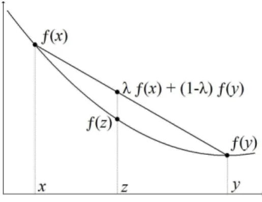
Definition 1.2.3 (Convex function [87]). A function f : X _{→ R defined on a}

convex set X ⊆ Rn _{is called convex if} _{∀x, y ∈ X, ∀λ ∈ [0, 1], it holds that f(z) ≤}

λf (x) + (1_{− λ)f(y), where z = λx + (1 − λ)y. If λ ∈ (0, 1) and ∀x 6= y f(z) <}

λf (x) + (1_{− λ)f(y) then f is called strict convex function.}

A graphical representation of a convex function is given in Figure1.3. It is

inter-esting to underline some facts: (i) if a function g(x) is convex, then the constraints

having the form g(x) _{≤ b, b ∈ R are convex. In general, g(x) ≥ b could be a}

non-convex constraint, even if g(x) is a non-convex function. In the case of g(x) non-convex,

the constraint g(x)≥ b is called reverse convex [240]; (ii) if g(x) is linear, g(x) O b,

where O_{∈ {≤, =, ≥} is a convex constraint; (iii) if the set of feasible solutions X is}

defined by convex constraints, then it is convex. We can now introduce the following theorem:

(23)

Figure 1.3: Convex function f

Theorem 1.2.4 (Property of optimal solutions for convex problems [87]).

Consider a convex problem, that is a problem stated in the form (1.1) where X _{⊆ R}n

is a convex set, and the objective function to be minimized f : X → R is a convex

function. Each local optimum is also a global optimum.

Another important concept, that is concavity, is strictly related to convexity.

More precisely, substituting_{≤ and < with ≥ and > in Definition} 1.2.3, we obtain

the definitions of concave and strict concave function. These concepts are useful in the case of MP problem stated as maximization problems. The role of convexity

and concavity in MP can be summarized by these facts [38]:

• A local minimum (maximum) of a convex (concave) function on a convex feasible region is also a global minimum (maximum).

• A local minimum (maximum) of a strict convex (concave) function on a convex feasible region is the unique global minimum (maximum).

1.2.1.2 Classes of mathematical programming problems

We can now propose a classification of the MP problems formulated in the very

general form (1.1). Remember that the set X is given by the bounds and kinds

(as integer, continuous, or discrete) of the variables, and by the constraints of the

problem, which are usually on the form g(x)_{≤ 0 or g(x) = 0.}

• Linear Programming (LP): the objective function and the constraints are lin-ear, and the variables are continuous;

• Mixed Integer Linear Programming (MILP or MIP): the objective function

and the constraints are linear, and at least one variable is integer;2

2_{Actually MILP is a special case of NLP, as the integrality of a variable x}

j can be expressed

by the nonlinear constraint sin(πxj) = 0. Nevertheless MILP is separated from NLP because there

exist specific techniques to solve integer problems, as shown in Section1.2.2.2. If all the variables are integer, sometimes ILP (Integer Linear Programming) is used in place of MILP to refer to the problem.

(24)

• convex Nonlinear Programming (cNLP): the objective function and the con-straints are convex with at least one of them being nonlinear, and the variables are continuous;

• Nonlinear Programming (NLP): at least one among the objective function and the constraints is nonlinear, and the variables are continuous;

• convex Mixed Integer Nonlinear Programming (cMINLP): the objective func-tion and the constraints are convex with at least one of them being nonlinear, and at least one variable is integer;

• Mixed Integer Nonlinear Programming (MINLP): at least one among the ob-jective function and the constraints is nonlinear, and at least one variable is integer.

We can further write the following relationships: LP_{⊂ MILP ⊂ cMINLP ⊂ MINLP}

and LP⊂ cNLP ⊂ NLP ⊂ MINLP. The meaning is that if a solver can be employed

for a given class of problems C, then it can also be employed for problems of all

the classes D _{⊂ C. For instance, a MINLP solver can be employed to solve a NLP}

problem, but a NLP solver working on a MINLP instance will ignore the integrality constraints on the variables. These relationships give also an intuitive idea about

the complexity of the problems of the different categories. In general D_{⊂ C means}

that D is easier to solve than C. Hence, LP problems are usually the easiest to solve, whereas MINLPs are the most difficult. Note that usually convex problems are easier to solve than nonconvex ones, since, in the former, local optima are also global optima, as explained earlier.

It is possible to go further into detail with the categorization of MP problems, but for this thesis the previous classification suffices. The clustering problems presented

in Chapter 2 are MINLPs and cMINLPs, and we reformulate them as MILPs. In

Chapter 3 the Packing Equal Circles in a Square (PECS) problem is an example

of nonconvex NLP problem, and it is reformulated into another nonconvex NLP

problem. Finally, the problems presented in Chapter 4 can be either MINLPs or

NLPs, and they are reformulated respectively as MILPs and LPs.

At this point, the most natural questions are the following: which are the tech-niques used to solve these MP problems, and how the fact that a problem falls into one of the categories presented above affects the choice of the solution method? This is the subject of the next section.

1.2.2 Approaches to solve mathematical programming problems

In this section we present a brief summary of the techniques employed to solve MP problems belonging to the different classes presented in the previous section. If not specified, the variables are considered to belong to R.

(25)

1.2.2.1 Linear programming

In a LP problem the constraints and the objective function are linear. In its standard form, a LP problem can be expressed as:

min cTx

s.t. Ax = b

x_{≥ 0,}

where cT _{is the n dimensional row vector of coefficients for the objective function, A}

is the m_{× n matrix constraints, b is the m dimensional column vector representing}

the right-hand side of the constraints, and x is the n dimensional column vector of the nonnegative variables of the problem. The feasible region of such a problem is a convex set called convex polyhedron, having a finite number of vertices (i.e., points which cannot be expressed as strict convex combination of two any other points of the polyhedron). If the polyhedron is bounded it is called polytope. The importance of this concepts in LP is that the optimal solution of a LP problem corresponds to a vertex of the polytope representing the feasible region. This has been the key observation at the base of the simplex algorithm, that is an algorithm which starts from a vertex of the polyhedron and moves to another adjacent vertex as long as the objective function improves. The procedure stops when the vertex representing the optimal solution is reached. This is the main idea, but a lot of details are missed (e.g., how to perform this move from a vertex to a better one, how to know if the optimal

vertex is found). For more informations, see [56,70]. Although this algorithm has

an exponential complexity in the worst case, it is efficient in practice. However, in 1979 Khachiyan proved that LP can be solved in polynomial time, proposing the ellipsoid method, that is an interior point algorithm. In 1984 Karmarkar proposed

a better polynomial time interior point method to solve LP problems [139]. The

interior point methods are algorithms that find the optimal solution by moving on the interior of the polytope representing the feasible region, and not on the vertices as the simplex method. Regarding the efficiency, it is not clear which one between the simplex and the interior point algorithm performs better, since it depends on the problem itself. As consequence, LP solvers like CPLEX implement both methods. LPs are important because a lot of real-world problems can be described in this way. Moreover, LPs arise during the solution process of other categories of MP problems, as for example MILPs.

1.2.2.2 Mixed integer linear programming

A MILP problem consists of a linear objective function and some linear constraints, where a subset of the variables are integer. In general solving a MILP problem

(26)

MILP problem can be obtained by relaxing the integrality constraints and solving the resulting LP problem (called continuous relaxation). Consider the MILP problem stated in the standard form as follows:

min cTx (1.2)

s.t. Ax = b (1.3)

x_{∈ X} (1.4)

∀i ∈ I xi∈ Z, (1.5)

where I is the set of indices of integer variables. Let us introduce the concept of unimodularity:

Definition 1.2.5 (Unimodularity [87]). A m_{×n matrix A, where m ≤ n, is called}

unimodular if for all m_{× m submatrices B of A it holds that det(B) ∈ {−1, 0, 1}.}

Suppose that the polyhedron defined by (1.3)-(1.4) is not empty and limited (i.e.,

it is a polytope). Then the Theorem 1.2.6holds.

Theorem 1.2.6 (Integrality of the vertices of the polyhedron [87]). Let the

m× n matrix A be unimodular and the m dimensional column vector b be integer

valued. The polyhedron associated to (1.3)-(1.4) has only integer vertices.

It is known that the optimal solution of a LP problem is found on a vertex of the polyhedron defined by the constraints of the problem. If we relax the integrality

constraints (1.5) of the MILP problem, and solving the corresponding LP produces

an integer solution, then this solution is optimal for the MILP problem. In other words, the unimodularity of the constraint matrix A together with the integrality of the components of the vector b is a sufficient condition for obtaining the optimal solution of the MILP problem by solving its continuous LP relaxation. In the case of

problems where the constraints (1.3) are casted in form of inequalities, the concept

of unimodularity has to be substituted with that of total unimodularity in order to preserve the property of having integer vertices of the polyhedron (the difference

with respect to the unimodularity of Definition1.2.5is that, for total unimodularity,

the property det B _{∈ {−1, 0, 1} must hold for all m × m square submatrices B of A).}

In the general case, however, the solution obtained by solving the continuous relaxation of a MILP problem is not integer, hence other approaches must be em-ployed. The main techniques are the following:

• Branch-and-Bound (BB) [148]: first the continuous relaxation of the MILP

problem is solved. The optimal solution of the continuous relaxation ˇx has in

general some components ˇxi, i∈ I which are not integer. Consider a fractional

component ˇxi . Two new problems are generated from the original one, the

(27)

constraint xi ≥ ⌈ ˇxi⌉. This step is called branching, and xi is the branching

variable. The two subproblems generated correspond to express that xi ≤

⌊ ˇxi⌋ or xi ≥ ⌈ ˇxi⌉, that cannot be formulated by means of a linear constraint.

Then the continuous relaxations of the two subproblems are solved. If each problem is represented by a node, each branching produces two children, and the resulting structure is a binary tree (usually called BB tree). For each node, after solving the corresponding continuous relaxation and obtaining the

solution ˇx, the process of branching and generation of the two child nodes is

iterated unless one of the following fathoming criteria holds: (i) ˇx is integer;

(ii) ˇx = +_{∞, i.e., the continuous relaxation of the problem is infeasible; (iii)}

cT_x_ˇ _{≥ c}T_x∗_{, where x}∗ _{is the best optimal integer solution found so far (it}

is set to +_{∞ at the beginning, and then updated each time a better integer}

solution is found). Note that cT_{x is a lower bound on the cost of the optimal}_ˇ

integer solution which can be obtained by all the subproblems generated by the current node, i.e., these subproblems cannot provide solutions better than

cT_{x. This is the reason why it is not needed to continue the branching of a}_ˇ

node if its continuous relaxation provides a solution that is worse than the best know integer solution. Two last details concern the choice of the branching variable, since in general there can be several variables in I which are not integer, and the rule to explore nodes in the BB tree. A possible method to select the branching variable is to take the one having the fractional part closest to 0.5, in order to reduce significantly the feasible region of both subproblems. Some well-known rules to select the node for performing the branching are a depth-first approach (where the node to process is the deepest node not yet explored), and a best-bound first approach (where the node to process is the

one presenting the lower value of cTx). When all the nodes are explored theˇ

BB returns the optimal solution x∗, if the problem is feasible.

• Cutting Plane [107]: the first step of this method is to solve the continuous

relaxation of the problem. Then, given a solution ˇx, one finds an inequality

which is satisfied by each integer feasible solution of the problem but not

by the current solution ˇx (separation problem). This inequality, called cut,

is adjoined to the MILP formulation and the continuous relaxation is solved again. This is repeated until the optimal solution is integer. Different types of cuts are provided in the literature. Some examples are represented by the

Chv´atal inequalities and the Gomory cuts.

• Branch-and-Cut [203,204]: the problem of the cutting plane approach is that

there can be several cuts that do not improve so much the current solution (tailing off). Thus, one can merge the BB and the cutting plane techniques. More precisely, at each node of the BB tree some cuts are adjoined to the model, in order to obtain a better lower bound (or ideally an integer solution),

(28)

and consequently to employ in a more profitable way the fathoming criteria. When the cuts become no more effective, the branching is performed. This technique improves in general the results provided by BB or cutting plane used separately.

Heuristics algorithm are also very important, since they provide good feasible so-lutions which can be used to speed-up exact methods. Some examples are presented in [28,68,88,89,106]

1.2.2.3 Nonlinear and convex nonlinear programming

Nonlinear problems can be defined as follows:

min f (x) (1.6)

s.t. _{∀i ∈ M g}i(x)≤ 0 (1.7)

x_{∈ X,} (1.8)

where M =_{{1, . . . , m} and at least one among g}i(x) and f (x) is a nonlinear function.

If there are no constraints on the variable, the problem is called unconstrained. Finding the optimal solution of a NLP problem is not as easy as for LP and MILP,

due to the nonlinearities and in general nonconvexities (in this case Theorem 1.2.4

could not hold, with the possible consequence of having several local optima which makes the search for the global optimum by the solver difficult).

There exist some necessary conditions for the optimality called

Karush-Kuhn-Tucker (KKT) [140,144], which must be satisfied by a solution x∗ of a NLP problem

to be a local optimum, and which are used by some NLP solvers. They can stated as follows:

Definition 1.2.7 (KKT conditions). Given a NLP problem in the form (1.6

)-(1.8), a feasible point x∗ ≥ 0 which respects some regularity conditions is a local

optimum only if there exist some multipliers µi,∀i ∈ M such that these conditions

hold:

∀i ∈ M gi(x∗)≤ 0 (primal feasibility)

µi≥ 0 (dual feasibility) ∇f(x∗) + m X i=1 µi∇gi(x∗) = 0 (stationarity)

∀i ∈ M µigi(x∗) = 0 (complementary slackness),

where the objective function f and the constraints gi are differentiable in x∗ and

the operator ∇ applied to a function express its gradient. Some of the most

(29)

(LICQ) and require the gradient of the constraints that are active at x∗ to be linearly

independent when evaluated at x∗.

In the case of convex objective function and constraints (that is a cNLP) a KKT point (i.e., a point which satisfies the KKT conditions) is a global optimum. Actually, this holds for a wider class of functions than convex ones, i.e., invex functions. For

more details about invex functions, see [27,65,122,123,180].

The main methods to solve NLPs are presented below. In the case of cNLPs the solution found is the global optimum. For nonconvex NLPs, some of these methods can be employed but there is not proof of global optimality for the solution found. To find an ǫ approximation of the global optimum for nonconvex NLPs, a possible

approach is presented in Section1.2.2.5.

• Line Search [23]: this is an iterative method to solve unconstrained NLPs.

If the solution at the interation t is xt_{, the main steps for obtaining the new}

solution xt+1 are: (i) find a descent direction, that is a vector representing the

direction along which the objective function value decreases; (ii) decide a step

size; (iii) let xt+1 be equal to xt _{after the move of a step along the discent}

direction; (iv) repeat points (i)-(iii) until ∇f(xt+1_{) is smaller than a given}

tolerance. There are several methods to decide the descent direction and the step size, e.g., gradient descent, Newton, Quasi-Newton, conjugate gradient.

• Trust Region [23]: this is another iterative method where a nonlinear

func-tion is not approximated in its whole domain, but only in a subset of the domain (called trust region) where the approximation is supposed to be good. This is done because the quality of the approximation of a nonlinear function near a given point could be not so good far from this point. The new solution

xt+1 is then searched within the trust region associated to the current solution

xt_{. There are different methods to decide the dimension of the trust region}

(defined by a step size), and the direction for the search.

• Penalty Function [23,53]: in this case the constraints are removed from the

problem and placed in the objective function in order to penalize solutions that do not respect the constraints. Thus, the problem to solve is an unconstrained problem.

• Interior Point [23,53]: this method tries to reach the optimal solution by

moving on the interior of the feasible region, unlike methods as the simplex for LPs, which moves on the boundary of the feasible region. This is done by means of barrier functions, which prevent leaving the feasible region.

• Sequential Quadratic Programming (SQP) [23,53]: differently from the

penalty function and interior point approaches, this method tries to solve the KKT conditions for the original NLP problem. This leads to a quadratic

(30)

problem, where the objective function, if nonlinear, is replaced by a quadratic approximation, and the nonlinear constraints are linearized. To obtain the optimal solution within a certain tolerance, a sequence of quadratic problems is solved.

1.2.2.4 Convex mixed integer nonlinear programming

To solve cMINLP problems the main approaches are the following:

• Branch-and-Bound [116]: this is the extension of the BB algorithm for MILP

to nonlinear problems. At each node of the BB tree, instead of solving the LP problem corresponding to the continuous relaxation of a MILP problem, a cNLP problem (which corresponds to the continuous relaxation of a cMINLP problem) is solved.

• Outer-Approximation [81]: this is an iterative method where at each

it-eration a MILP relaxation of the cMINLP problem is solved (the nonlinear constraints are replaced by linear approximations). Then, the solution ob-tained is used to fix the integer variables of the cMINLP problem, and the corresponding cNLP relaxation is solved. The solution of the cNLP problem is used to generate some cuts to add to the MILP formulation, and the process is repeated. Solving the MILP problem provides a lower bound and solving the cNLP problem provides an upper bound on the solution of the cMINLP problem. When these two bounds are equal within a certain tolerance, then the optimal solution is found.

• Generalized Benders Decomposition [102]: this method is based on the

Benders decomposition technique previously proposed by Benders for MILP. It can be seen as a variant of the outer-approximation method, where the MILP relaxation is not obtained by linearizing all the nonlinear constraints, but all these linearized constraints are combined to obtain a single constraint which is adjoined to the model (surrogate relaxation). As a consequence, the solution of this MILP problem provides in general a worse (i.e., lower) lower bound with respect to the outer-approximation method, leading to a larger number of iterations needed to obtain the solution, but on the other hand each MILP problem can be solved faster.

• Extended Cutting Plane [248]: this method works by solving iteratively a

MILP relaxation of the original cMINLP problem, where the linearization of the most violated nonlinear constraint by the optimal solution is adjoined to the MILP formulation which is solved at the next iteration.

• LP/NLP based Branch-and-Bound [208]: this technique extends the

(31)

the outer-approximation method, a MILP relaxation is solved, but only once. In fact, this problem is solved by means of the BB as described for MILPs, with a main difference. Whenever an integer solution is found at the current node of the BB tree, it is used to fix the integer variables of the cMINLP problem yielding a cNLP problem. The solution of this cNLP problem is then used to derive some cuts that are adjoined to the MILP formulation at the current node, and the BB solution process continues.

As for MILPs, heuristics are very important for cMINLPs, since they can be used to find good feasible solutions and thus accelerate the algorithms presented above.

Some examples are presented in [1,29,34,35].

1.2.2.5 Mixed integer nonlinear programming

In the general case a MINLP problem is nonconvex. In this case, the use of the techniques employed for cMINLPs would provide a local optimum without proof of global optimality (unless the MINLP problem is reformulated as a cMINLP problem,

but this is not always possible [153]). For obtaining global optimal solutions for

nonconvex MINLPs, one can employ an ε-approximation algorithm called spatial

Branch-and-Bound (sBB). Several variants exist, among which [5,26,83,91,154,217,

232,242]. Couenne [26], or BARON [220] are examples of solvers implementing

sBB. Given a constant ε > 0, the sBB recursively generates a binary search tree,

some leaf node of which contains a feasible point x∗ for which f (x∗) differs by at

most ε from the globally optimal value of the objective function (with a slight abuse

of notation, we refer to x∗ as the ε approximation of the optimal solution instead of

the real global optimum).

A very important step for each sBB algorithm is the convex relaxation of the original nonconvex problem. The solution of the convex relaxation provides a lower bound for the value of the optimal solution in the original problem. Some examples

of convex relaxations are presented in Chapter4, and more details about how these

convex relaxations are computed are provided in [156]. At each iteration of the

algorithm, convex relaxations restricted to particular sub-regions of space are solved, and a lower and an upper bound to the optimal value of the objective function can be assigned to each sub-region. A global optimum relative to the sub-region is identified when lower and upper bounds are very close together. More precisely, a generic node

a of the sBB tree contains a formulation restricted to some region, or box Ba_{as well}

as a lower bound value f (ˇxa) relative to the parent node. All along the sBB run,

the following data are maintained:

• the search tree, encoded in some efficiently accessible form; • the best solution so far (also called the incumbent).

(32)

1.3. Reformulations 15

The following steps are performed at each node a. At the beginning, f (x∗) = +_∞

and x∗ = (+_{∞, . . . , +∞).}

1. Range tightening: techniques such as Optimization-Based Bounds Tightening

(OBBT) [154] (where the range of variables is reduced in order to avoid the

exploration of regions which do not contain any feasible point) and

Feasibility-Based Bounds Tightening (FBBT) [24] (where using the constraints of the

problem and interval analysis the bounds of the variables are tightened) are

employed in order to attempt to reduce the width of Ba _{in view to obtaining}

a tighter lower bound.

2. Computation of a lower bound f (ˇxa): this is done by means of solving a convex

relaxation of the problem restricted to a region Ba.

3. Pruning by bound: if f (ˇxa) ≥ f(x∗) then the box Ba cannot contain optima

better than the incumbent. Go to Step8.

4. Computation of an upper bounding solution (ˆxa, f (ˆxa)): it is obtained using a

local NLP solver on the problem at the node, with (ˇxa, f (ˇxa)) as a starting

point.

5. Incumbent evaluation: if f (ˆxa) < f (x∗) then let (x∗, f (x∗))← (ˆxa, f (ˆxa)).

6. Pruning by optimality: if f (ˆxa)−f(ˇxa) < ε, then ˆxais an ε-approximate global

optimum within the box Ba; further refinements will not yield better optima.

Go to Step 8.

7. Branching: select a variable and a value for branching: this consists in creating

two subnodes a1, a2of a, one with the subproblem where the branching variable

is constrained between its lower range end and the branching value, and the other between the branching value and its upper range end; several heuristics

exist for selecting branching variable and value [26].

8. Choice of next node: again, several heuristic methods exist. The most popular seems to be the choice of the node with the highest associated upper bound, insofar as it intuitively offers the best promise of improving the incumbent.

In the end, x∗ is the optimal solution. A proof of finite convergence of the sBB to

an ε-approximation of a global optimum is given in [241].

1.3 Reformulations

In the literature, different definitions of reformulation are presented. For instance, Sherali proposed the following definition:

(33)

Definition 1.3.1 (Sherali’s reformulation [228]). A reformulation in the sense

of Sherali of an optimization problem P (with objective function fP) is a problem

Q (with objective function fQ) such that there is a pair (σ, τ ) where σ is a bijection

between the feasible region of Q and that of P , and τ is a monotonic univariate

function with fQ = τ (fP).

This definition is really strict, excluding from the class of reformulations all the cases where there does not exist a bijection σ between the feasible region of the reformulated problem Q and that of the original one P .

An alternative definition of reformulation is given by Audet et al. in [15]:

Definition 1.3.2 (Audet’s reformulation [15]). Let PAand PB be two

optimiza-tion problems. A reformulaoptimiza-tion in the sense of Audet B(_{·) of P}Aas PB is a mapping

from PA to PB such that, given any instance A of PA and an optimal solution of

B(A), an optimal solution of A can be obtained within a polynomial amount of time. In this case the definition excludes nonpolynomial time reformulations, which could be carried out in a reasonable amount of time, and it includes all the poly-nomial time reformulations even if very slow in practice. Moreover, there is no guarantee of preserving local or global optima.

A third definition of reformulation (also called auxiliary problem) is due to Liberti [157]:

Definition 1.3.3 (Liberti’s reformulation [157]). Any problem Q that is related

to a given problem P by a computable formula f (Q, P ) = 0 is called an auxiliary problem (or reformulation) with respect to P .

Starting from this definition, four different types of reformulations are presented

in [157]. We introduce them more in detail in the next section, except for the

approximation reformulation that is not used in this thesis because an approximation just leads to one of the other types of reformulation for some limiting value of a parameter.

1.3.1 Classification of reformulations

Following the Definition1.3.3, reformulations can be classified as:

• exact or opt-reformulations: transformations preserving all optimality proper-ties;

• narrowings: transformations preserving at least one global optimum;

• relaxations: transformations based on dropping constraints, variable bounds or types;

(34)

1.3. Reformulations 17

Given a problem, one could first try to obtain an exact reformulation, in order to have an alternative formulation which could be possibly easier to solve but preserving all optimality properties. If the problem is still hard to solve, and it presents several global optima, one can then try to obtain a narrowing. For very difficult problems, or for specific algorithms, it may be necessary to employ a relaxation, eliminating some constraints (e.g., integrality of variables, bounds on variables or some inequalities). Hence, the optimal solution of the relaxation provides a guaranteed bound to the optimal objective function value (lower bound in case of minimization, upper bound in case of maximization). In the worst case, one must employ approximations, which do not provide any guarantee on optimality.

We now introduce more formally these first three categories. We indicate as F(P ), L(P ) and G(P ) respectively the feasible region, the set of local optima, and the set of global optima for the problem P .

1.3.1.1 Exact reformulations

Exact reformulations are auxiliary problems that preserve all optimality information. Definition 1.3.4 (Exact reformulation). Q is an exact reformulation (or

opt-reformulation) of P if each local optimum l_{∈ L(P ) corresponds to a local optimum}

l′ _{∈ L(Q) and each global optimum g ∈ G(P ) corresponds to a global optimum}

g′ ∈ G(Q).

In other words, this type of reformulation preserves both local and global opti-mality informations. Exact reformulations can be chained (i.e., applied in sequence) to obtain other exact reformulations.

1.3.1.2 Narrowings

Narrowings are auxiliary problems where some global optima are removed, but at least one is kept.

Definition 1.3.5 (Narrowing reformulation). Q is a narrowing of P if each

global optimum g′ ∈ G(Q) corresponds to a global optimum g ∈ G(P ).

It turns out that there can be global optima in_{G(P ) without any corresponding}

global optimum in G(Q). Narrowings are useful in presence of problems exhibiting

many symmetries. For instance, the PECS problem presented in Chapter 3 has

a high degree of symmetry, and the search tree associated to the sBB algorithm becomes very large. Hence, the time to reach the leaves (which represent the optimal solutions) can be prohibitive. In this case a narrowing, which can be obtained by adjoining Symmetry Breaking Constraints (SBCs) to the original formulation, can dramatically reduce the completion time.

(35)

Note that exact reformulations can be seen as a special case of narrowings. More-over, a narrowing chained to another narrowing leads another (more complex) nar-rowing, and a narrowing chained to an exact reformulation provides a narrowing.

1.3.1.3 Relaxations

A relaxation of a problem P is an auxiliary problem Q of P whose optimal objec-tive function value is a bound (lower in the case of minimization, upper in the case of maximization) for the optimum objective function value of the original problem. Such bounds are mainly used in BB type algorithms, which are the most common exact or ε-approximate (for a given ε > 0) solution algorithms for MILPs, non-convex NLPs and MINLPs. Moreover, these bounds can be used to evaluate the

performance of heuristic algorithms without an approximation guarantee [72], or to

guide heuristics [207].

Definition 1.3.6 (Relaxation). Q is a relaxation of P if _{F(P ) ⊆ F(Q), and}

considering minimization problems P and Q where fP and fQ are respectively their

objective functions, then∀x ∈ F(P ), fQ(x)≤ fP(x).

In other words, a problem Q is a relaxation of P if both the feasible region of P is contained into the feasible region of Q and the objective function of Q provides better (or equal) value than the objective function of P when evaluated in the points of the feasible region of P .

There are different kinds of relaxations. For instance the elimination relaxation takes place when we simply drop some constraints (as in the continuous relaxation for integer problems, where the integrality constraints on the variables are dropped). In the surrogate relaxation a set of constraints is replaced by a linear combination of them. In the Lagrangian relaxation a set of constraints is removed from the model but the objective function is modified in order to penalize solutions which does not respect these constraints. A more detailed presentation of these relaxations can be found in [206].

Exact reformulations and narrowings are special types of relaxations. Further-more, relaxations can be chained to obtain other relaxations, and chains of relax-ations with exact reformulrelax-ations and narrowings are themselves relaxrelax-ations.

1.4 Contributions

The main goal of this thesis is to investigate problems to show the impact of the

reformulations presented in Section 1.3. Rather than focusing on the design of

specific algorithms for a given problem, we try to improve the MP model used to describe that problem, obtaining alternative models (reformulations), and comparing them with respect to the original formulation. This comparison very often takes into account the computation time, even if in some cases other parameters are considered

(36)

1.4. Contributions 19

(e.g., the quality of the partitions obtained by the algorithms proposed in Section

2.3, the effect of the SBCs on the results obtained by the local solver in Chapter 3,

the value of the upper bound, the best solution found and the size of the BB tree for the PECS instances whose solution time reached the time limit, as presented in

Table3.6).

In Chapter 2 we introduce the problem of clustering in general and bipartite

graphs as example of application of exact reformulations. We show that alternative formulations lead to an improvement of the computational time needed to get the solution. This chapter also contains an important contribution to clustering (albeit not strictly related to reformulations). Some of the models presented in that chapter contain simple SBCs, thus leading to narrowing reformulations. A more exhaustive

analysis of narrowings is performed in Chapter3, where we study the PECS problem.

We consider this problem as example of the application of narrowings, because it involves a high degree of symmetry. We characterize the symmetric structure of the problem, and then we propose SBCs to remove some of the previously detected symmetries. Indeed, the problem is very difficult and we were not able to improve the best-known solutions (in terms of cost of the objective function), since the best results for large instances are often obtained by heuristics, and not by means of a MP model solved by a general MINLP solver (we employ the solver Couenne for our tests). However, the impact of SBCs is very clear when comparing the number of sBB nodes and computational time for the original formulation and the narrowings.

Finally, Chapter 4 refers to relaxations. More precisely, we introduce problems

with multilinear terms, and we propose two relaxations: one (called primal) obtained by replacing each multilinear term with a new variable and several constraints, and another one obtained using a dual representation. Even if the theory underlying this two relaxations is well-known, it is interesting to compare them empirically. It appears from our computational tests that the dual approach is more stable and outperforms the primal one in terms of computational time when the size of problems increases. This can have a considerable impact, since pratically every sBB code uses primal relaxations.

(37)

(38)

Part I

An application of exact

reformulations

(39)

(40)

23 This part of the thesis is devoted to the problem of clustering in unweighted general and bipartite graphs, and it presents two main contributions. First, we introduce the concept of modularity as measure of quality for clustering, and we present an existing hierarchical divisive heuristic for finding high modularity partitions for a given graph,

described in [47]. We propose several reformulations for the MP model used by this

heuristic, which decrease the computational time. The proposed reformulations are mostly exact reformulations, even if there is also a SBC, which leads to narrowing

reformulations. However, applications of narrowing will be studied in Chapter 3.

After that, we adapt the hierarchical divisive heuristic and the reformulations to

bipartite graphs. This first part is mainly based on the work presented in [45,58].

In the second part we study clustering from another point of view, not strictly related with reformulations. More precisely, one can obtain partitions into clusters by specifying conditions that each cluster must respect. Starting from a previously

proposed condition, namely the strong criterion of Radicchi et al. [210], we modify

it obtaining the almost-strong criterion, that produces more informative partitions. We first present two MP models to describe the problem of finding partitions in the strong and almost-strong sense. However, due to the size of these formulations, we propose a specific algorithm to find these partitions. This second part is based on

(41)

(42)

Chapter

2

Clustering in general and bipartite

graphs

Graphs have been intensively used in several domains to represent complex

sys-tems [198]. For instance, the metabolic networks studied in biology and

bioinfor-matics [115,205], social networks [105] and other applications in informatics, as

recommender systems [6] or the World Wide Web [90]. One of the most important

tasks is to identify the structure of such graphs, and in particular to find (gener-ally disjoint) subsets of vertices, called communities or clusters, where each cluster contains vertices that are more likely to be pairwise connected with other vertices in the same cluster than with those belonging to other clusters. The detection of communities in graphs has many applications. The identification of relationships between users and products can be employed to develop targeted marketing pro-grams or to design recommender systems that can suggest items to users, which is very useful for business purposes. Clustering is useful in biology, for example in the analysis of graphs representing interaction between proteins, to detect groups of proteins having similar functions within a cell. Another application arises from information retrieval, where clusters represent documents related to the same topic. This is a helpful support to search engines in the World Wide Web.

It often appears that complex and real-world graphs have a hierarchical structure, i.e., a cluster can be seen as a set of smaller clusters, and so on. Hierarchy in complex

systems has been defined by H. A. Simon as follows [231]:

By a hierarchic system, or hierarchy, I mean a system that is composed of interrelated subsystems, each of the latter being, in turn, hierarchic in structure until we reach some lowest level of elementary subsystem.

Consider again the example taken from information retrieval: a cluster representing a set of documents related with a general topic (for example, cars), might contain smaller clusters, each one of them representing a more specific subject related with

(43)

the topic of the parent cluster (for instance, different brands of cars like Renault, Citr¨oen, Mazda, and so on). We might further suppose that each cluster representing a brand can be itself divided into other clusters, each one representing a specific model of car of that brand. Thus, clustering can also be employed to detect the hierarchical structure of a graph.

There are several methods to detect clusters in graphs, and they can be divided into three broad categories:

• Heuristic algorithms. In this case the clusters are found by a heuristic, as for example the hierarchical divisive heuristic proposed by Girvan and

New-man [105], where the edge with largest betweenness (which is the number of

pair of nodes for which the edge belongs to the shortest path joining them) is iteratively removed, and clusters correspond to connected components ob-tained each time a cluster is split in two. This heuristic therefore proceeds from an initial (trivial) partition in a single cluster containing all vertices to a final partition in which each cluster contains a single vertex.

• Maximization (or minimization) of an objective function. Among a large num-ber of examples, one of the most known is the modularity, initially proposed as a stopping rule for the divisive heuristic mentioned above and later con-sidered as an independent criterion; modularity is presented in detail in

Sec-tion 2.2. Other well-known criteria are the k-way cut [54,118], the

normal-ized cut [33,230], the ratio cut [118], the modularity density and its

vari-ants [132,152], and strength maximization subject to strong or weak

con-straints on the communities [78,185]. More recently, several promising criteria

have been put forward, e.g., information compression [216], maximum

likeli-hood and the expectation maximization algorithm [17], and the constant Potts

model [239].

• Constraints to be satisfied by each community. Several such constraints have

been proposed; the early ones are reviewed in the book [245]. They include

the cliques, in which every pair of vertices must be joined by an edge, the k-regular graph in which the indegree of each vertex must be at least k, and

the LS (Luccio-Sami) set [174], i.e., a set of vertices S such that each of its

proper subsets has more ties to its complement within S than to the outside of S. These three criteria tend to be too stringent and/or too difficult to compute, except on the smallest graphs. Two other well-known criteria, which express the intuitive idea of a community, have been proposed by Radicchi et

al. [210]: a subset S of vertices of a graph forms a community in the strong

sense if the number of neighbors of each vertex within S is larger than the number of neighbors outside S. A set of vertices S forms a community in the weak sense if the sum, for all of its vertices, of the difference between

(44)

2.1. Definitions and notation 27

the number of neighbors within S and the number of neighbors outside S is positive. Recently, weakened versions have been proposed, in which instead of comparing the numbers of neighbors within and outside the community, one compares the numbers of neighbors within a community, and outside that

community but within another specific community [132]. In Section 2.3 we

propose a weakened version of the concept of community in the strong sense,

which leads to the definition of community in the almost-strong sense [44].

The main contributions of this chapter are the following: first, in Section 2.2.1 we

introduce the hierarchical divisive heuristic presented in [47], and we propose some

reformulations for the MP model used by this heuristic, which considerably reduce

the computational time. In Section 2.2.2 we extend the divisive heuristic for the

case of bipartite graphs, and we employ techniques similar to those presented in

Section2.2.1to obtain good MP models for this heuristic. Finally, Section2.3deals

with a contribution not related with modularity maximization and reformulations.

Starting from the definition of community in the strong sense presented in [210], we

propose a weakened version, yielding the so called community in the almost-strong sense, which appears to provide partitions into communities much more informative than the ones obtained by the original community in the strong sense criterion. In order to compare these criteria, two specific algorithms for finding partitions in the strong and almost-strong sense are proposed.

2.1 Definitions and notation

We denote a general graph, or network, by G = (V, E), where V is the set of

n vertices, and E is the set of m edges joining pairs of vertices. A vertex vj is

represented by a point and an edge ei,j = {vi, vj} by a line joining its two end

vertices vi and vj. The shape of this line does not matter, only the presence or

absence of an edge is important. A loop ei,i = {vi, vi} is an edge for which both

end vertices coincide. In a simple graph, there is at most one edge between any pair

of vertices, and no loops. The degree ki of a vertex vi ∈ V is the number of edges

incident with vi, and it can be split into two parts: the indegree kini or number of

neighbors of vi within its community and the outdegree kouti or number of neighbors

of vi outside its community. The adjacency matrix A = (ai,j) of G is a square n by

n matrix such that ai,j = 1 if vertices vi and vj are joined by an edge, and equal

to 0 otherwise. A subgraph GS = (S, ES) of a graph G = (V, E) induced by a set

of vertices S _{⊆ V is a graph with vertex set S and edge set E}S equal to all edges

with both vertices in S. A set S of vertices is a clique if all pairs of vertices of S are

joined by an edge, i.e., _∀vi ∈ S ki =|S| − 1. A set S induces a k-regular graph if

every vertex of S has at least k neighbors within S, where k is a parameter.

Applications of Reformulations in Mathematical Programming

HAL Id: pastel-00746083

https://pastel.archives-ouvertes.fr/pastel-00746083

Programming

Alberto Costa

To cite this version:

Applications of Reformulations in

Mathematical Programming

Th`

ese pr´

esent´

ee pour obtenir le grade de

DOCTEUR DE L’´

ECOLE POLYTECHNIQUE

par

Alberto Costa

Soutenue le 18 septembre 2012 devant le jury compos´

e de:

Abstract

R´esum´e

Acknowledgements

Acronyms

Contents

Chapter

1

Introduction

1.1

Motivations

1.2

Mathematical programming

1.3

Reformulations

1.4

Contributions

Part I

An application of exact

reformulations

Chapter

2

Clustering in general and bipartite

graphs

2.1

Definitions and notation