Study and modeling of separation methods H2S from methane, selection of a method favoring H2S valorization

HAL Id: tel-01764942

https://pastel.archives-ouvertes.fr/tel-01764942

Submitted on 12 Apr 2018

HAL is a multi-disciplinary open access

archive for the deposit and dissemination of sci-entific research documents, whether they are pub-lished or not. The documents may come from teaching and research institutions in France or abroad, or from public or private research centers.

L’archive ouverte pluridisciplinaire HAL, est destinée au dépôt et à la diffusion de documents scientifiques de niveau recherche, publiés ou non, émanant des établissements d’enseignement et de recherche français ou étrangers, des laboratoires publics ou privés.

Study and modeling of separation methods H2S from

methane, selection of a method favoring H2S valorization

Hamadi Cherif

To cite this version:

Hamadi Cherif. Study and modeling of separation methods H2S from methane, selection of a method favoring H2S valorization. Chemical and Process Engineering. Université Paris sciences et lettres, 2016. English. �NNT : 2016PSLEM074�. �tel-01764942�

Soutenue par Hamadi

CHERIF

le 08 Décembre 2016

h

Dirigée par Christophe COQUELET

Paolo STRINGARI

h

COMPOSITION DU JURY :

M. Vincent GERBAUD

Chemical Engineering Laboratory of Toulouse, Président

M. Eric MAY

University of Western Australia, Rapporteur 

Mme. Laura PELLEGRINI

Politecnico di Milano, Examinatrice M. Denis CLODIC

Société Cryo Pur, Examinateur M. Christophe COQUELET Mines ParisTech, Examinateur M. Paolo STRINGARI

Mines ParisTech, Examinateur M. Joseph TOUBASSY Société Cryo Pur, Invité

Ecole doctorale

n°432

SCIENCES DES METIERS DE L’INGENIEUR

Spécialité

ENERGETIQUE ET GENIE DES PROCEDES

Etude et modélisation de méthodes de séparation du méthane et de H

2

S

Study and modeling of separation methods of H

2

S from methane

THÈSE DE DOCTORAT

de l’Université de recherche Paris Sciences et Lettres 

PSL Research University

3

Acknowledgements

I am grateful to Prof. Denis Clodic, supervisor of this thesis for the suggestions that helped to shape my research skills and for the responsibility he granted to me. Without him, this dissertation would not have been possible.

I would like to thank my supervisors Prof. Christophe Coquelet and Dr. Paolo Stringari, for their continuous support, excellent supervision and guidance. Without them, this thesis would not have been possible.

I express my gratitude to Prof. Eric May from the University of Western Australia and Prof. Vincent Gerbaud from the Chemical Engineering Laboratory of Toulouse, for their patience while reading this thesis.

I would like to thank Prof. Laura Pellegrini for her hospitality and disponibility during my stay in Politecnico di Milano within "Group on Advanced Separation Processes & GAS Processing". It was an opportunity to grow on both a personal and professional level.

I would also thank Dr. Joseph Toubassy, project leader at Cryo Pur Company, for being interested in my work, for the various disscussion we had and for his technical aid.

I thank all the staff in CTP and Cryo Pur Company for their presene, their support and their advices. I would like to recognize the support of my parents Jaafar and Wassila through all these years.

4

Table of contents

Abstract ... Erreur ! Signet non défini.

Nomenclature ... 7

List of figures ... 9

List of tables ... 11

General introduction ... 13

Chapter 1: From biogas to biomethane ... 17

1.1. Introduction ... 18

1.2. Biogas utilization ... 19

1.2.1. Direct combustion ... 19

1.2.2. Combined heat and power ... 19

1.2.3. Injection into the natural gas grid ... 19

1.2.4. Vehicle fuel ... 19

1.3. Biogas composition ... 20

1.3.1. Household and industrial waste ... 20

1.3.2. Sludge from sewage water treatment plants ... 21

1.3.3. Agricultural and agro-industrial waste ... 21

1.4. Environmental and economic issues ... 23

1.5. From biogas to liquid biomethane ... 24

1.6. Conclusion ... 25

Chapter 2: Thermodynamic aspects of biogas ... 26

2.1. Introduction ... 26

2.2. Thermodynamic properties of pure component present in biogas ... 27

2.2.1. Hydrogen sulfide ... 27

2.2.2. Carbon dioxide... 28

2.2.3. Methane ... 29

2.3. Thermodynamic properties of the gas mixture (biogas) ... 32

2.3.1. Phase equilibrium behavior of biogas ... 32

2.3.2. Density and dynamic viscosity of biogas ... 34

2.3.3. Thermal conductivity of biogas ... 35

2.3.4. Thermal capacities ... 36

5

2.5. Conclusion ... 38

Chapter 3: From molecules to the process ... 39

3.1. Introduction ... 39 3.2. Absorption technology ... 40 3.2.1. Physical solvents ... 41 3.2.2. Chemical solvents ... 44 3.2.3. Hybrid solvents ... 47 3.2.4. Gas-liquid contactors ... 47 3.3. Adsorption technology ... 50 3.3.1. Mechanism of adsorption ... 51

3.3.2. Materials used for H2S adsorption ... 52

3.3.3. Factors affecting the adsorption ... 54

3.3.4. Adsorption isotherms ... 55

3.3.5. Adsorption processes ... 58

3.4. Membranes technology ... 59

3.5. Cryogenic technology ... 64

3.6. Choice of the separation process ... 66

3.7. Conclusion ... 69

Chapter 4: Industrial demonstrator description ... 71

4.1. Introduction ... 71

4.2. General presentation of the BioGNVAL pilot plant ... 73

4.3. The operating principle of the BioGNVAL subsystems ... 76

4.3.1. Desulfurization subsystems ... 76

4.3.2. Dehumidification and siloxanes icing subsystem ... 79

4.3.3. Carbon dioxide capture subsystem ... 79

4.3.4. Biogas liquefaction subsystem ... 79

4.4. Experimental results concerning the removal of hydrogen sulfide by chemical absorption using sodium hydroxide ... 81

4.5. Conclusion ... 83

Chapter 5: Hydrodynamic study of gas-liquid countercurrent flows in structured packing

columns ... 84

5.1. Introduction ... 84

5.2. Theoretical principles ... 85

5.2.1. Billet and Schultes model ... 86

6

5.2.3. Delft model ... 92

5.3. Models evaluation ... 93

5.3.1. Pressure drop and liquid holdup ... 94

5.3.2. Effective interfacial area ... 96

5.4. Changes made to Billet and Schultes model and results ... 98

5.5. Conclusion ... 105

Chapter 6: Comparison of experimental and simulation results for the removal of H

2

S from

biogas by means of sodium hydroxide in structured packed columns ... 106

6.1. Introduction ... 108

6.2. Aspen Plus® simulations ... 108

6.2.1. Validation of the Temperature-Dependent Henry’s constant for CH4 – H2O, CO2 – H2O and H2S – H2O systems ... 109

6.2.2. Validation of heat capacity for carbon dioxide ... 112

6.2.3. Validation of liquid density of NaOH – H2O ... 113

6.2.4. Validation of liquid viscosity of NaOH – H2O ... 114

6.2.5. Validation of surface tension of NaOH – H2O ... 117

6.2.6. Validation of chemical parameters ... 118

6.2.7. Simulation results ... 122

6.3. Conclusion ... 127

Chapter 7: Modeling hydrogen sulfide adsorption onto activated carbon ... 128

7.1. Introduction ... 128

7.2. Operating conditions of the adsorption column for the removal of hydrogen sulfide ... 129

7.3. Breakthrough curve modeling ... 131

7.3.1. Estimation of mass transfer coefficients ... 132

7.3.2. Modeling of breakthrough curves ... 136

7.4. Conclusion ... 142

7

Nomenclature

a Specific geometric packing surface area m2_/m3

A Constant used for the calculation of pressure drop -

ae Effective interfacial area m2

b Length of the corrugation base m

B Constant used for the calculation of pressure drop -

CFl Specific packing constant for calculation of hydrodynamic parameters at

flooding point -

Ch Specific packing constant for hydraulic area -

CL Specific packing constant for mass transfer calculation in liquid phase -

Clp Specific packing constant for calculation of hydrodynamic parameters at

loading point -

Cp Specific packing constant for pressure drop calculation -

CV Specific packing constant for mass transfer calculation in gas phase -

DV Gas-phase diffusion coefficient m2/s

d Packing diameter m

dh Hydraulic diameter m

dhV Diameter of the gas flow channel m

dp Particle diameter m

f Approach to flood -

Fc Gas capacity factor (m/s) (kg/m3)0.5

Fc,lp Gas capacity factor at loading point (m/s) (kg/m3)0.5

FrL Liquid Froude number -

Fl Enhancement factor for pressure drop calculation -

Ft Correction factor -

FSE Surface enhancement factor for effective interfacial area calculation -

fw Wetting factor -

g Gravitational constant m/s2

geff Effective gravitational constant m/s2

h Corrugation height m

hL Liquid holdup m3/m3

hL,Fl Liquid holdup at flooding point m3/m3

hL,lp Liquid holdup at loading point m3/m3

hL,pl Liquid holdup in preloading region m3/m3

K Wall factor -

kG Gas-phase mass transfer coefficient m/s

kL Liquid-phase mass transfer coefficient m/s

L Liquid mass flow kg/h

M Molar mass kg/mol

nFl Exponent for calculation of liquid holdup at flooding point -

nlp Exponent for calculation of liquid holdup at loading point -

P Pressure Pa

Pc Critical pressure Pa

Pe Peclet number -

ReL Liquid Reynolds number -

ReV Gas Reynolds number -

ReV,e Effective Reynolds number for gas phase

ReV,r Relative Reynolds number for gas phase

8

Sc Schmidt number - Sh Sherwood number - T Temperature K TB Boiling temperature K Tc Critical temperature K

uL Superficial liquid velocity m/s

uL,e Effective liquid velocity m/s

uL,lp Superficial liquid velocity at loading point m/s

uV Superficial gas velocity m/s

uV,e Effective gas velocity m/s

uV,Fl Superficial gas velocity at flooding point m/s

uV,lp Superficial gas velocity at loading point m/s

V Gas mass flow kg/h

WeL Liquid Weber number -

z Unit length m

𝑑𝑃

𝑑𝑧 Pressure drop Pa/m

(𝑑𝑃

𝑑𝑧)𝑑 Dry pressure drop Pa/m

(𝑑𝑃

𝑑𝑧)_𝑝𝑙 Pressure drop in preloading region Pa/m

αL Liquid flow angle °

γ Solid – liquid film contact angle °

δ Liquid film thickness m

ε Void fraction -

ζDC Coefficient for losses caused by direction change -

ζGG Coefficient for gas/gas friction losses -

ζGL Coefficient for gas/liquid friction losses -

θ Corrugation angle °

µL Dynamic viscosity of the liquid phase kg/m.s

µV Dynamic viscosity of the gas phase kg/m.s

νL Kinematic viscosity of the liquid phase m2/s

ξbulk Direction change coefficient in the bulk zone -

ξGG Gas/Gas friction coefficient -

ξGL Gas/Liquid friction coefficient -

ξwall Direction change coefficient near the wall -

ρL Liquid density kg/m3

ρV Gas density kg/m3

σL Surface tension of the liquid phase N/m

σW Surface tension of water N/m

φ Fraction of the flow channel occupied by the liquid phase -

Ψ0 Resistance coefficient for dry pressure drop calculation -

ΨFl Resistance coefficient for pressure drop calculation at flooding point -

ΨL Resistance coefficient for wet pressure drop calculation -

Ψ’L Resistance coefficient for wet pressure drop calculation -

ψlp Resistance coefficient for pressure drop calculation at loading point -

9

List of figures

Fig. 1: Distribution of final energy consumption in France [1] ... 13

Fig. 2: Distribution of production of renewable energies by sector [1] ... 14

Fig. 3: Biogas primary production in 2013 [2] ... 15

Fig. 4: Simplified diagram of production of biomethane ... 18

Fig. 5: Example of biogas utilization by Cryo Pur® Company [9]... 20

Fig. 6: Vapor pressure of the main components present in biogas ... 31

Fig. 7: Pressure – Temperature equilibrium behavior for the CH

4

– CO

2

system [29] ... 32

Fig. 8: Pressure – Temperature equilibrium behavior for the CH

4

– H

2

S system [30] ... 33

Fig. 9: Biogas density as a function of temperature ... 34

Fig. 10: Biogas viscosity as a function of temperature ... 35

Fig. 11: Thermal conductivity of biogas as a function of temperature ... 36

Fig. 12: Heat capacity at constant pressure of biogas as a function of temperature ... 37

Fig. 13: Heat capacity at constant volume of biogas as a function of temperature ... 37

Fig. 14: Two-film theory [36] ... 41

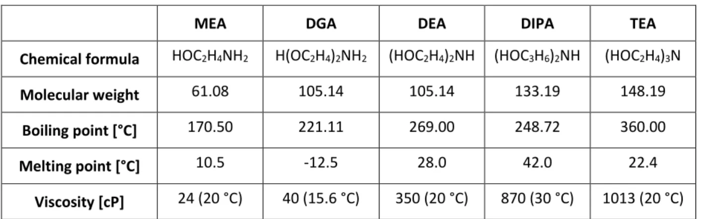
Fig. 15: Chemical structure of some alkanolamines [43] ... 46

Fig. 16: Main gas-liquid contactors [48] ... 49

Fig. 17: Schematic representation of a packed column ... 49

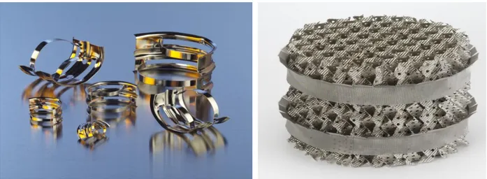
Fig. 18.a: Random packing Nutter Ring [Sulzer] ... 50

Fig. 18.b : Structured packing Mellapak [Sulzer] ... 50

Fig. 19: Transport mechanism of the adsorbate molecules on the adsorbent surface ... 52

Fig. 20: Shapes of commercial activated carbons [53]... 53

Fig. 21: Effect of temperature on some adsorbents [57] ... 54

Fig. 22: Classification of adsorption isotherms [IUPAC] ... 56

Fig. 23: Skarstrom cycle stages and pressure variations [68] ... 59

Fig. 24: Schematic representation of a membrane [71] ... 60

Fig. 25: Diagram of the main types of membranes [75] ... 62

Fig. 26: The geometric configurations of membrane contactors [76] ... 63

Fig. 27: Most technologies used for the purification and upgrading of biogas [International

Energy Agency] ... 66

Fig. 28: Comparison of investment costs of different biogas purification and upgrading

technologies [88] ... 69

Fig. 29: BioGNVAL demonstrator located at Valenton water treatment plant [9] ... 72

Fig. 30: Schematic representation of Cryo Pur® system [9] ... 73

Fig. 31: Simplified flowsheet of the BioGNVAL pilot plant [9] ... 74

Fig. 32: Schematic diagram of the absorption subsystem for elimination of hydrogen sulfide

[9] ... 77

Fig. 33: Piping and instrumentation diagram of adsorption subsystem for the removal of

hydrogen sulfide [9] ... 78

Fig. 34: Carbon dioxide antisublimation [9] ... 80

Fig. 35: Variation of the H

2

S content at the inlet and at the outlet of the absorption column

... 81

Fig. 36: Variation of the biogas temperature at the inlet of the demonstrator and at the

outlet of the absorption column ... 82

Fig. 37: Observation of the desorption phenomenon of H

2

S ... 83

Fig. 38.a: Pressure drop evolution in a packing column ... 86

10

Fig. 39.a. Pressure drop evaluation for liquid load u

L

= 20.5 m/h ... 95

Fig. 39.b. Liquid holdup evaluation for liquid load u

L

= 20.5 m/h ... 95

Fig. 40.a. Prediction of effective interfacial area by Billet and Schultes model for the system

Air / Kerosol 200 ... 96

Fig. 40.b. Prediction of effective interfacial area by SRP model for the system Air / Kerosol

200 ... 97

Fig. 40.c. Prediction of effective interfacial area by Delft model for the system Air / Kerosol

200 ... 97

Fig. 41. Liquid holdup and pressure drop with an Air – Water system using Flexipac® 350Y

packing ... 102

Fig. 42. Liquid holdup and pressure drop with an Air – Kerosol 200 system using Flexipac®

350Y packing ... 104

Fig. 43: Flowsheet of the absorption process simulated using Aspen Plus® ... 108

Fig. 44: Henry coefficients for CH

4

– H

2

O system ... 110

Fig. 45: Henry coefficients for CO

2

– H

2

O system ... 111

Fig. 46: Henry coefficients for H

2

S – H

2

O system ... 111

Fig. 47: Comparison between model and experimental data for heat capacity for carbon

dioxide ... 112

Fig. 48: Deviation between experimental and calculated results of carbon dioxide heat

capacity... 113

Fig. 49: Comparison between model and experimental data for liquid density of NaOH – H

2

O

... 113

Fig. 50: Deviation between experimental and calculated results of liquid density ... 114

Fig. 51: Comparison between model and experimental data for liquid viscosity of NaOH –

H

2

O ... 116

Fig. 52: Deviation between experimental and calculated results of liquid viscosity ... 116

Fig. 53: Comparison between model and experimental data for liquid phase surface tension

of 5 wt% NaOH aqueous solution ... 117

Fig. 54: Deviation between experimental and calculated results of surface tension ... 118

Fig. 55: Comparison of results of equilibrium constant for reaction R.18 ... 120

Fig. 56: Comparison of results of reaction rate constant for reaction R.24 ... 121

Fig. 57: Deviation between experimental and calculated results of reaction rate constant

(R.24) ... 121

Fig. 58: Influence of the liquid flow on the absorption of hydrogen sulfide ... 123

Fig. 59: Influence of gas flow rate on the pressure drop ... 124

Fig. 60: Deviation between experimental and calculated results of pressure drop ... 124

Fig. 61: Influence of the concentration of NaOH in the removal of H

2

S and CO

2

... 125

Fig. 62: Influence of the temperature of liquid in the absorption of hydrogen sulfide ... 126

Fig. 63: Deviation between experimental and calculated results of H

2

S concentration leaving

the packing column ... 126

Fig. 64: Influence of relative humidity in the adsorption of hydrogen sulfide using Airpel Ultra

DS [53] ... 130

Fig. 65: Schematic representation of an adsorption column [122] ... 131

Fig. 66: Influence of Langmuir equilibrium parameters on adsoption sites occupied ... 137

Fig. 67: Breakthrough curve simulated for H

2

S molar percentage of 5 % ... 141

Fig. 68: Breakthrough curve simulated for H

2

S molar percentage of 7.5 % ... 141

11

List of tables

Table 1. Concentration requirements before biogas liquefaction [8] ... 19

Table 2. Composition and characterization of household waste [13] ... 21

Table 3. Production yields for agricultural and agro-industrial substrates [14] ... 22

Table 4. Biogas composition depending on the type of substrate [14] ... 23

Table 5. Tolerances in impurities for the use of liquid biomethane as vehicle fuel [14] ... 24

Table 6. Thermo-physical properties of hydrogen sulfide [19] ... 28

Table 7. Thermo-physical properties of carbon dioxide [19] ... 29

Table 8. Thermo-physical properties of methane [19] ... 30

Table 9. Constants used by Antoine Equation for the calculation of H

2

S, CO

2

and CH

4

vapor

pressures ... 31

Table 10. Solubility of the main compounds of biogas in water [39] ... 42

Table 11. Properties of physical solvents [40] ... 43

Table 12. Solubility of gases in physical solvents at 25 °C and 0.1 MPa [41] ... 44

Table 13. Physical properties of some chemical solvents [43] ... 45

Table 14. Classification of main gas-liquid contactors [48]... 48

Table 15. Criteria to differentiate between physical and chemical adsorption [49] ... 51

Table 16. Equations governing adsorption isotherm models, and their linear forms [67] ... 57

Table 17. The membrane materials used by manufacturer [71] ... 60

Table 18. Classification of membrane separation processes [73] ... 61

Table 19. Distribution of membranes according to pore size [IUPAC] ... 62

Table 20. Characteristics of the different geometries of membranes [76] ... 64

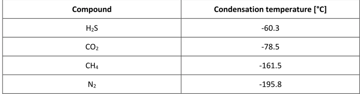
Table 21. Condensation or solidification temperatures, at atmospheric pressure, for the

different compounds present in biogas ... 65

Table 22. Effect of temperature on the abatement of volatile organic silicon compounds.... 65

Table 23. Comparison of the different biogas purification and upgrading technologies ... 67

Table 24. Performances, costs, advantages and disadvantages of separation processes [87] 68

Table 25. Conditions and composition of the raw biogas treated by BioGNVAL pilot plant ... 75

Table 26. conditions of passage from one subsystem to another [9] ... 75

Table 27. Sensitivities of measurement tools ... 81

Table 28. Constants for the Billet and Schultes model [98] ... 87

Table 29. Effective interfacial area in packing columns using Billet and Schultes model [98] 87

Table 30. Liquid holdup and velocities at loading and flooding point [99] ... 88

Table 31. Liquid holdup in preloading and loading regions [98] ... 89

Table 32. Pressure drop in packing columns using Billet and Schultes model [98] ... 89

Table 33. Effective interfacial area in packing columns using SRP model [96] ... 90

Table 34. Liquid holdup in packing columns using SRP model [101] ... 91

Table 35. Pressure drop in packing columns using SRP model [96] ... 91

Table 36. Pressure drop in preloading region using Delft model [97] ... 93

Table 37. Physical properties of the systems tested [100] ... 94

Table 38. Dimensions of Flexipac® 350Y [100] ... 94

Table 39. Deviation between predictive models and experimental data ... 96

Table 40. Changes made to calculate liquid holdup ... 99

Table 41. Changes made to calculate Pressure drop for liquid density less than 900 kg.m

-3

_{. 99}

Table 42. Changes made to calculate Pressure drop for liquid density higher than 900 kg.m

-3

... 100

12

Table 43. Statistical deviation between the modified model and experimental data for

pressure drop and liquid holdup predictions ... 104

Table 44. Comparison between modified correlations and experimental data for the

prediction of pressure drop in a structured packing column ... 105

Table 45. Coefficients used by Aspen Plus® to calculate Henry’s constant ... 109

Table 46. Coefficients used by Harvey to calculate Henry’s constants ... 110

Table 47. Values of the constants used by Equation (87) to calculate the heat capacity of

carbon dioxide ... 112

Table 48. Coefficients used in the calculation of the equilibrium constant ... 119

Table 49. Coefficients used in the calculation of the equilibrium constant of Reaction (R.6)

... 119

Table 50. Parameters k and E for kinetic-controlled reactions [119] ... 120

Table 51. Details of the simulated process ... 122

Table 52. Influence of liquid flow rate on the pressure drop ... 123

Table 53. Activated carbon properties used for this study [53] ... 129

Table 54. Biogas composition and operating conditions of the adsorption process ... 132

Table 55. Sherwood number estimation [123] ... 133

Table 56. Estimation of the binary diffusion coefficients [135] ... 134

Table 57. Equations used to estimate internal diffusion coefficients ... 135

Table 58. Estimation of dimensionless numbers and diffusion coefficients ... 135

Table 59. Boundary and initial conditions of the system ... 138

13

General introduction

Recent decades were accompanied by economic growth and prosperity for humanity. This growth gained from oil and natural gas production has been accompanied by an environmental pollution that may trigger irreversible changes in the environment with catastrophic consequences for humans. Moreover, issues related to the reduction of fossil reserves are still relevant, and the global primary energy demand is increasing, pushing the international community to pursue the development of renewable energies.

The law on energy transition plans to reduce the share of fossil fuel consumption in France to 30 % in 2030, while the share of renewable energy should be increased to 23 % in 2020 and 32 % in 2030 against 16.1 % in 2012 as shown in the Fig. 1 [1].

Fig. 1: Distribution of final energy consumption in France [1]

Renewable energy is derived directly from natural phenomena. It takes many forms: sunlight, wind, wood heat, water power … The main renewable energies are: wind power, wave power, geothermal energy, solar energy, biomass, firewood and hydropower …

According to the French Ministry of Energy [1], primary production of renewable energy rises to 22.4 Million tonnes of oil equivalent (Mtoe) in 2012. The distribution of renewabale energies production by sector is depicted in Fig. 2.

Among renewable energies, biogas is a possibility. It is storable, transportable, not intermittent and substitutable for fossil energies. These strengths justify the consolidation of this emerging sector and the preparation of its future development by ambitious public policies. The European primary energy production from biogas reached 5901 kilotonnes of oil equivalent (ktoe) in 2007, 7500 ktoe in 2008, 10086 ktoe in 2011 and 13379 ktoe in 2013.

14

Fig. 2: Distribution of production of renewable energies by sector [1]

Biogas production is at the heart of the policy priorities for 2020, the European Union aims for a production that will cover 50 % of transport sector needs. Biogas is a growing sector. Fig. 3 provides a quick review of biogas production in Europe in 2013 [2].

Generally, this gas composed of methane and carbon dioxide, also contains other compounds as water, ammonia, volatile organic compounds and hydrogen sulfide.

Biogas can be valued in several applications such as production of heat and/or electricity, feed for fuel cells, injection into the natural gas grid and production of liquefied bio-methane. This last application presents an environmental and economic benefits. With hydrogen fuel, liquefied bio-methane is one of the best fuel for the reduction of carbon dioxide emissions with a reduction potential up to 97 % compared to Diesel. It can effectively reduce emissions of greenhouse gases and the pollution, responsible for 42000 premature deaths annually in France [3].

Biofuels (2.4) Hydropower (5) Firewood (10) Heat pumps (1.4) Wind power (1.3) Urban waste (1) Biogas (0.4) Solar energy (0.4) Agricultural waste (0.3) Geothermal energy (0.1) Others (3.6)

15

Fig. 3: Biogas primary production in 2013 [2]

16

Liquefied bio-methane requires very low temperatures which may lead to solidification of impurities and thus facilities malfunctions. These impurities must be separated from the biogas. This implies implementation of a purification process to remove from the raw biogas all unwanted substances in order to maximize its methane content. In particular, the complete desulfurization of biogas is peremptory in order to ensure an optimal operation and a high purity of other compounds to valorize, such as carbon dioxide. Moreover, the presence of hydrogen sulfide in the wet biogas, is a poison for installations. In case of leakage, the presence of hydrogen sulphide in the biogas characterized by a rotten egg smell can be dangerous for operators working on the site. Hence, the need to remove all traces of this compound. Several technologies are used for the removal of H2S as adsorption on

microporous solids, membrane technology, biological processes and absorption by means of liquid solvents.

The choice of the technique to implement is related to various parameters. The most important are the flow rate of biogas and hydrogen sulfide concentrations to treat. The solution must also respond to various economic, environmental and energetic imperatives as cost which must be reasonable, the threshold to reject which must be respected in an energy-efficient process. Therefore, there is no universal treatment method.

In this thesis, the choice fell on the use of a cryogenic method in order to combine biogas upgrading and biomethane liquefaction. The removal of H2S will be performed upstream of the process either by

reactive absorption using an aqueous solution of sodium hydroxide (NaOH) in a structured packed column or by adsorption using activated carbon. These two technologies will be tested and compared in order to choose the most effective and the most suitable for the process set up.

Experiments were performed on a industrial pilot plant developed by Cryo Pur® company called “BioGNVAL”. This pilot plant treats 85 Nm3_{/h of biogas from waste water treatment plant, which}

contains around 20 – 100 ppm of H2S.

For absorption technology, the hydrodynamic of flows in structured packing columns was studied in order to develop a model able to predict realistically the key hydrodynamic parameters as pressure drop, liquid holdup and transition points but also effective interfacial area and global mass transfer coefficients.

The remainder of the study is based on simulations using Aspen Plus® V8.0 to study realistically the effectiveness of a structured packed column which uses sodium hydroxide as a chemical solvent for the selective removal of hydrogen sulfide from biogas. Results were compared with data from BioGNVAL pilot plant.

Finally, the dynamic aspect of the adsorption phenomenon is modeled, by predicting the breakthrough curve in the case of an adsorption column used for the removal of H2S.

17

Chapter 1: From biogas to biomethane

Résumé :

Après une introduction générale posant le contexte de la production de biogaz dans le paysage énergétique mondial, le premier chapitre est une introduction à la problématique de son obtention et de son usage sous une version raffinée en biométhane.

Le biogaz est produit par méthanisation lorsque des matières organiques sont décomposées dans des conditions bien définies et en absence d’oxygène. Il est constitué principalement de méthane et de dioxyde de carbone mais aussi de quantités variables de vapeur d’eau, de sulfure d’hydrogène et d’autres composés polluants. Afin de pouvoir utiliser le biogaz comme carburant pour véhicule, il doit être épuré en séparant le dioxyde de carbone et les autres composés contaminants du biogaz pour augmenter au maximum sa teneur en méthane.

Il existe différentes technologies utilisées dans le domaine du traitement des gaz. Les plus utilisées sont : l’absorption, l’adsorption, la technologie membranaire, la cryogénie, le traitement biologique et l’oxydation. Aujourd'hui, d'autres technologies sont développées telles que la biocatalyse, la photocatalyse et le plasma froid. Pour le moment, le manque d'informations à leur sujet limite leur application industrielle [18].

18

1.1. Introduction

Anaerobic digestion may be defined as the natural process of degradation by microorganisms under controlled conditions and in the absence of oxygen. This degradation results in the production of a gas mixture saturated with water outlet of the digester called biogas.

Anaerobic digestion is the result of four biochemical steps in which large carbon chains are converted into fatty acids and alcohols. These four steps are: Hydrolysis, acidogenesis, acetogenesis, methanogenesis [4].

 Hydrolysis

It takes place at the beginning of the fermentation and makes use of exo-enzymes in order to decompose the organic matter into simple substances.

 Acidogenesis

During this step, volatile fatty acids are formed. Carbon dioxide and hydrogen are also formed, they are used by microorganisms during the production of methane according to the chemical Reaction (R.1) shown below. The reaction enthalpy is about -567 kJ.mol-1 _[5].

𝐶𝑂₂+ 4 𝐻₂ → 𝐶𝐻₄+ 2 𝐻₂𝑂 (R.1)

 Acetogenesis

This stage involves the production of acetate, an indispensable substrate for the synthesis of methane.

 Methanogenesis

This last step results in the production of methane. It is ensured by the methanogenic bacteria, which can only use a limited number of carbon compounds, including acetate responsible for 70 % of methane production according to the chemical Reaction (R.2) shown below. The reaction enthalpy is about -130 kJ.mol-1 _[5].

𝐶𝐻₃𝐶𝑂𝑂𝐻 + 𝐻₂𝑂 → 𝐶𝐻₄+ 𝐻₂𝐶𝑂₃ (R.2)

The biogas needs to be purified and upgraded, which means that impurities are removed or valorized in order to produce a gas rich in methane called biomethane. There is a number of technologies available for this purpose as water scrubbing, membranes and pressure swing adsorption.

Fig. 4: Simplified diagram of production of biomethane

Gas upgrading unit

Biogas

Biomethane (CH

4

)

By-product(s) as CO

2 CH4 CO2 H2O N2 O2 H2S VOCs NH3 Siloxanes

19

1.2. Biogas utilization

Biogas can be used in several applications. Sometimes it could be used raw, but almost always it has to be upgraded or as a minimum cleaned from its H2S content because the presence of this compound

in the biogas even at very low concentrations could damage the installations.

Biogas can be used in all applications designed for natural gas such us production of heat and electricity known as combined heat and power (CHP), production of chemicals and/or proteins, fueling internal combustion engines and fuel cells, it may also be used as vehicle fuel or injected in the natural gas grids.

1.2.1. Direct combustion

The simplest method of biogas utilization is direct combustion. The biogas burner can be installed in heaters for production of hot water and hot air, in dryers for various materials, and in boilers for production of steam for process heat or power generation [6]. Another limited application involves absorption heating and cooling to provide chilled water for refrigeration and hot water for industrial processes.

These applications based on direct combustion do not require a high gas quality.

Biogas can also be used to fuel internal combustion engines to supply electric power for pumps, blowers, elevator and conveyors, heat pumps and air conditioners [7].

1.2.2. Combined heat and power

Another application for biogas is CHP which involves the production of two or more forms of energy, generally electricity and thermal energy. This latter is generally the most used today but it could be a problem because the need of heat varies with season, and during summer for example, unused biogas is flared.

1.2.3. Injection into the natural gas grid

Upgrading of biogas to biomethane with a gas quality similar to natural gas and injecting it into the natural gas grid is an efficient way to integrate biogas into the energy sector. It allows the transport of large volume of biomethane and its utilization in wide areas where population is concentrated.

1.2.4. Vehicle fuel

Today, there is a big interest in using biogas as a vehicle fuel. But for this utilization, the raw biogas must be purified which means that contaminants are removed from biogas, and upgraded which means that CO2 is eliminated leading to a raise in the energy content of biogas. Finally, the biomethane

needs to be liquefied by chilling it to very low temperatures (≈ -161 °C at atmospheric pressure). In order to prevent corrosion and solid formation, some requirements concerning component concentrations are needed before liquefaction. They are presented in Table 1. The H2S content must

be lower than 4 ppm. This quantity is not in direct relation with corrosion or solidification aspects. This requirement ensures a high quality of biomethane and avoids odor problems caused by the presence of hydrogen sulfide.

Table 1. Concentration requirements before biogas liquefaction [8]

Compounds Maximum concentration

CO2 25 ppm

H2S 4 ppm

20

Fig. 5 shows an example of use of biogas after its purification and upgrading using the Cryo Pur® system developed by Cryo Pur® Company.

Fig. 5: Example of biogas utilization by Cryo Pur® Company [9]

1.3. Biogas composition

The composition of biogas depends mainly on the type of substrates which are segmented according to their origin. The following classification is commonly used:

 Household and industrial waste.

 Sludge from sewage water treatment plants.  Agricultural and agro-industrial waste.

1.3.1. Household and industrial waste

To treat this type of waste, they are buried in landfill sites. The anaerobic conditions created by the landfill are sufficient to induce methanogenesis.

Biogas production from this type of waste is characterized by variations of flow rates and composition due to the variation of the feedstock. This biogas production is also dependent on the progression of degradation of waste, moisture and temperature. These parameters are not the same on the entire degradation zone leading to variations in the composition of biogas produced from the same landfill. This variability phenomenon is also noticeable on the concentration of methane in biogas which varies around 15 % during a year [10]. Two factors explain this: the high biological activity in summer and the rise of temperature. These conditions complicate the valorization of this type of biogas.

Household waste sorting improves the yield of biogas production. This process by which waste is separated into different elements achieves higher yields compared to unsorted waste. The difference may reach 100 m3_{/t [11].}

Household and industrial wastes are not all fermentable. The share of these fermentable wastes represents 45 % maximum [12].

21

Table 2. Composition and characterization of household waste [13]

Compounds Composition [wt. %] Dry matter [wt. %] Dry organic matter [wt. %]

Putrescible 33.0 44 77 Papers 11.7 68 80 Cardboards 12.0 70 80 Various incombustible 8.5 90 1 Tetra brik 8.5 70 60 Glasses 5.4 98 2 Plastic 4.9 85 90 Green waste 4.5 50 79 Textiles 4.2 74 92 Metals 3.7 90 1 Special waste 2.0 90 1 Various fuels 1.6 85 75

1.3.2. Sludge from sewage water treatment plants

Biological treatment of urban wastewater is a widespread process which generates significant amounts of activated sludge. In order to stabilize these latter, an anaerobic degradation is used. It provides a solution to the storage and treatment of sludge.

A small part of the produced biogas ensures 100 % of the energy needs of the wastewater treatment plant. The by-products of anaerobic digestion, as the digestate can be valorized via fertilization and amendment of farmland.

Today, the injection into the natural gas grid of biomethane issued from sludge of wastewater treatment plant is subject to strong demand from local authorities. According to the French Ministry of Ecology, Sustainable Development and Energy, by 2020, more than 60 wastewater treatment plants could be provided with the necessary facilities for energy recovery of waste to allow the injection of 500 GWh/year of biomethane into the national gas grid, which is equivalent to the annual consumption of more than 40000 households [1].

Unlike the treatment of household and industrial waste, anaerobic digestion of sludge from wastewater treatment plants is a controlled process conducted under optimal conditions for biogas generation.

1.3.3. Agricultural and agro-industrial waste

According to the European renewable energies Observatory [2], France has about 60 million tons of organic material that can be valued in biogas. These agricultural wastes are divided into two groups: liquid effluents and solid waste. For liquid effluents, dry matter and dry organic matter rates influence the production of biogas, as shown in Table 3. Digesters used for biogas production from agricultural and agro-industrial wastes are optimized systems, regulated and stable. According to Boulinguiez [14], the composition of biogas from digesters varies with an amplitude of ± 5 % during the year.

22

Table 3. Production yields for agricultural and agro-industrial substrates [14]

Substrates Dry matter [wt. %]

Dry organic matter [wt. %]

Production yield [m3_/t

of dry organic matter]

Production yield [m3_/t of substrate] Pig manure 6 to 25 75 to 80 300 to 450 22 to 60 Cow manure 8 to 30 80 to 82 350 to 700 21 to 168 Chicken manure 10 to 60 67 to 77 300 to 800 20 to 180 Horse manure 28 25 500 35 sheep manure 15 to 25 80 to 85 350 50 to 74 Grass silage 26 to 80 67 to 98 500 to 600 87 to 440 Hay 86 to 93 83 to 93 500 356 to 432 corn straw 86 72 500 310 Foliage 85 82 400 279 Sorghum 25 93 700 162 Helianthus annuus 35 88 750 231 Distillation residues 12 90 430 77 Brewery waste 15 to 21 66 to 95 500 50 to 100 Vegetable waste 5 to 20 76 to 90 600 23 to 108 oleaginous residues 92 97 600 536 Fruit residues 40 to 50 30 to 93 450 to 500 60 to 232 press cake 88 93 5550 450 slaughterhouse waste 15 80 to 90 450 58 bakery waste 50 80 to 95 450 665 Shortening waste 99 99 1200 1117

Table 3 shows that shortening (Alimentary fat) is the substrate with the highest methanogenic potential.

Assuming complete reaction without formation of by-products, Buswell Equation (1) shows that the theoretical yield of methane production may be estimated from the base elemental composition of a substrate [15].

23

𝐶_𝑐𝐻_ℎ𝑂_𝑜𝑁_𝑛𝑆_𝑠+ 𝑦 𝐻₂𝑂 → 𝑥 𝐶𝐻₄+ (𝑐 − 𝑥) 𝐶𝑂₂+ 𝑛 𝑁𝐻₃+ 𝑠 𝐻₂𝑆 𝑥 = 1 8 (4 𝑐 + ℎ − 2 𝑜 − 3 𝑛 − 2 𝑠) 𝑦 =1 4 (4 𝑐 − ℎ − 2 𝑜 + 3 𝑛 + 3 𝑠) (1)

The composition of biogas shown in Table 4 is defined according to the main types of substrates previously presented.

Table 4. Biogas composition depending on the type of substrate [14]

Compounds Unit Biogas from household and industrial waste Biogas from wastewater treatment plants Agricultural biogas CH4 % mol. 40 - 55 65 - 75 45 - 75 CO2 % mol. 25 - 30 20 - 35 25 - 55 N2 % mol. 10 0 – 5 0 - 5 O2 % mol. 1 - 5 0.5 0 - 2

NH3 % mol. Traces Traces 0 - 3

COV mg.Nm-3 _{< 2500 < 3000 < 1500}

H2S mg.Nm-3 < 3000 < 4000 < 10000

1.4. Environmental and economic issues

Biogas is a very interesting energy from an ecological and economic point of view.

The environmental interest of reducing CO2 emissions coincides with the approaches adopted to

the production and consumption of renewable energies. The environmental impact of production and valorization of biogas is easily demonstrable.

From an economic point of view, digesters allow to value all the types of substrates discussed in the previous section at attractive cost. In addition, the digest that was recovered at the outlet of the digester could be valorized as fertilizer.



Environmental issues

Anaerobic digestion is a natural phenomenon that rejects methane which is 23 times more potent as a greenhouse gas than carbon dioxide [16]. The simple conversion by combustion of CH4 into CO2

reduced to 8 % the initial potential of greenhouse gas from biogas, emitted directly into the atmosphere. Carbon dioxide footprint could be further improved when the biogas is purified and upgraded.

Moreover, the fossil energy used massively today releases large amounts of CO2 and it is not an

inexhaustible resource. The valorization of biogas is therefore interesting for environmental protection by saving fossil fuels and avoiding methane emissions into the atmosphere.

24



Economic issues

The economic feasibility of a biogas sector depends mainly on the composition of the biogas. The methane concentration in a biogas produced from household and industrial wastes is low as seen in Table 4. The CH4 concentrations do not exceed 55 %. Moreover, the biogas produced can vary

over time and it contains large amount of minor compounds, complicating biogas valorization. Biogas production from this type of waste is expected to be limited in future years in Europe. Restrictions and European standards are becoming more stringent, which makes the use of this source, unprofitable [12]. The most advanced biogas applications as vehicle fuel production or injection into the natural gas grid are hardly possible from this source, which requires advanced purification treatments.

Considering an anaerobic digestion unit treating 50000 t/year of household waste, the total costs vary between 50 and 95 €/t while the incomes do not exceed 30 €/t [14].

The economic balance of biogas production within wastewater treatment plants depends on the size and savings made on the sludge. This stable and controlled anaerobic digestion process is financially viable.

The wastewater treatment plant “Aquapol” situated in Grenoble, France treats 88 000 000 m3 _of

wastewater each year which is equivalent to 8000 dry tons of sludge processed per year. Part of the produced biogas is used for internal energy needs of the plant (8 GWh/year). The other part (14 GWh/year) will be injected in the natural gas grid after purification and compression [17].

The establishment of biogas purification process from agricultural waste is particularly attractive due to the reliability of the resource. The introduction of energy crops among the substrates improves the performance of anaerobic digestion giving a new economic aspect for the production of biogas.

1.5. From biogas to liquid biomethane

An advanced purification of biogas allows achieving an adequate quality threshold for use as vehicle fuel. The major step of this treatment is the separation of CO2, in addition to

dehumidification, desulfurization, reduction of oxygen and the removal of trace compounds in biogas. Qualities and tolerances in impurities, for the production of liquid biomethane to be used as vehicle fuel are listed in Table 5.

Table 5. Tolerances in impurities for the use of liquid biomethane as vehicle fuel [14]

Compounds Unit Liquid biomethane used as vehicle fuel

Methane – CH4 wt. % > 96 Carbone dioxide – CO2 wt. % < 3 Oxygen – O2 wt. % < 3 Water – H2O mg.m-3 < 30 Hydrogen sulfide – H2S mg.m-3 < 5 Total sulfur mg.m-3 _{< 120} Organosulfur mg.m-3 _{< 15} Hydrocarbons mg.m-3 _{< 200}

Critical size of particles μm < 1

Liquid biogas can be produced using a cryogenic upgrading technology, based on differences in condensation temperature for different compounds. It can also be produced by mean of a conventional technology connected with a small-scale liquefaction plant. When using the first method,

25

the carbon dioxide comes as a by-product which could be used in external applications bringing in extra income to the biogas upgrading unit.

The environmental benefits provided by the passage from the diesel to biomethane are impressive. Used as a fuel, Bio-LNG enables a considerable reduction of polluting emissions and represents a genuine alternative to diesel:



Zero emission of fine particles responsible for 42000 premature deaths annually in France.



-70 % NOx emissions.



-90 % CO2 emissions.



-99 % hydrocarbons emissions.



-50 % noise pollution.

Bio-LNG is a renewable energy produced from waste which makes it neutral in terms of greenhouse gas emissions. Its use allows the decarbonization of the energy mix. Bio-LNG is the only sustainable solution for long-distance haulage operated by heavy goods vehicles.

1.6. Conclusion

Biogas is produced when organic material is decomposed under anaerobic conditions. The main constituents are methane and carbon dioxide. To be able to use the raw biogas as a vehicle fuel it must be purified and upgraded, which means that impurities and CO2 respectively, are separated. There are

a number of available upgrading technologies and the most commonly used are:



Absorption



Adsorption



Membranes



Cryogenic technology

Other technologies exist such as oxidation and biological treatment. These techniques are known in the field of gas treatment. Today other technologies are being developed such as biocatalysis, photocatalysis and cold plasma. For the moment, the lack of information about them limits their industrial application [18].

The choice of the technology to be used to purify, upgrade and liquefy the biogas requires the knowledge of the thermodynamic properties of biogas and the representation of phase equilibrium. These thermodynamics aspects of biogas will be discussed in the next chapter.

26

Chapter 2: Thermodynamic aspects of biogas

Résumé :

Le choix de la technologie à utiliser pour purifier et liquéfier le biogaz exige la connaissance des propriétés thermodynamiques du biogaz.

Ce chapitre recense les propriétés thermodynamiques des fluides qui sont essentielles pour concevoir et optimiser les technologies de purification de biogaz. Il montre aussi que les propriétés thermophysiques du biogaz dépendent fortement de sa composition, en particulier des concentrations de méthane et de dioxyde de carbone. La présence de composés à faibles concentrations comme l’azote ou l’hydrogène sulfuré pourrait modifier les propriétés physiques du biogaz. Par exemple, les gaz d'enfouissement comprennent de petites quantités d'azote et d'oxygène qui affectent le comportement de phase du système CH4 – CO2.

27

2.1. Introduction

Thermodynamics can be used as a powerful tool for setting and evaluating processes used for purification and upgrading of biogas. Therefore, this study will focus on the thermodynamic investigation of biogas. It will present the thermodynamic properties of pure compounds and of the gas mixture (biogas) at a pressure of 1.103 bar. This pressure is considered because the biogas treated in the experimental part (Chapter 4) comes from the wastewater treatment plant at a pressure slightly above atmospheric pressure in order to avoid air infiltration into the biogas pipe.

2.2. Thermodynamic properties of pure component present in biogas

Biogas refers to a mixture of different molecules of gases as seen in Table 4. The thermodynamic aspects of the main components of biogas will be presented in this section.

2.2.1. Hydrogen sulfide

Hydrogen sulfide is a colorless gas with the characteristic foul odor of rotten eggs. It is very poisonous, corrosive, flammable and explosive. Its olfactory threshold varies between 0.7 and 200 g.m -3_{, depending on the sensitivity of each individual. The olfactory sensation is not proportional to the}

concentration of H2S in the air because it is possible that the smell felt at very low concentrations is

attenuated or disappeared at high concentrations.

Hydrogen sulfide is created following the bacterial decomposition of organic matter in the absence of oxygen, such as in swamps and sewers. It also appears in volcanic gases and hot springs. Other sources of hydrogen sulfide are the industrial processes used in the oil and natural gas sectors, sewage treatment plants and factories producing pulp and paper …

28

Table 6. Thermo-physical properties of hydrogen sulfide [19]

Properties Unit Value

Molar mass g.mol-1 _34.08

Auto-ignition temperature °C 270

Solubility in water (1.013 bar

and 0 °C) vol/vol 4.67

Solid phase

Melting point °C -85.7

Latent heat of fusion (1.013

bar at melting point) kJ.kg

-1 _69.73

Liquid phase

Boiling point at 1.013 bar °C -60.3

Vapor pressure at 20 °C bar 17.81

Liquid phase density (1.013 bar

at boiling point) kg.m

-3 _949.2

Latent heat of vaporization

(1.013 bar at boiling point) kJ.kg

-1 _546.41

Gas phase

Gas phase density (1.013 bar

and 15 °C) kg.m

-3 _1.45

Viscosity (1.013 bar and 0 °C) Pa.s 1.13 x 10-5

Thermal conductivity (1.013

bar and 0 °C) mW.m

-1_.K-1 _15.61

Specific volume (1.013 bar and

25 °C) m

3_.kg-1 _0.7126

Heat capacity at constant

pressure (1.013 bar and 25 °C) kJ.mol

-1_.K-1 _0.0346

Heat capacity at constant

volume (1.013 bar and 25 °C) kJ.mol

-1_.K-1 _0.026

Critical point

Critical temperature °C 99.95

Critical pressure bar 90

Critical density kg.m-3 _347.28

Triple point

Triple point temperature °C -85.45

Triple point pressure bar 0.232

2.2.2. Carbon dioxide

Carbon dioxide is a colorless and odorless gas which is naturally present in the Earth's atmosphere. The concentration of carbon dioxide in the atmosphere reached 405 ppm at the end of 2016, against only 283 ppm in 1839.

Carbon dioxide is produced by all aerobic organisms when they metabolize carbohydrate and lipids to produce energy by respiration [20]. It is also produced by burning fossil fuels such as coal, natural gas and oil. Significant amounts of CO2 are also released by volcanoes.

29

Table 7. Thermo-physical properties of carbon dioxide [19]

Properties Unit Value

Molar mass g.mol-1 _44.01

Concentration in air Vol % 0.0405

Solubility in water (1.013 bar

and 0 °C) vol/vol 1.7163

Solid phase

Melting point °C -56.57

Latent heat of fusion (1.013

bar at melting point) kJ.kg

-1 _204.93

Solid phase density kg.m-3 ₁₅₆₂

Liquid phase

Boiling point °C -78.45

Vapor pressure at 20 °C bar 57.291

Liquid phase density (19.7 bar

at -20 °C) kg.m

-3 _1256.74

Gas phase

Gas phase density (1.013 bar

and 15 °C) kg.m

-3 _1.87

Viscosity (1.013 bar and 0 °C) Pa.s 1.37 x 10-5

Thermal conductivity (1.013

bar and 0 °C) mW.m

-1_.K-1 _14.67

Specific volume (1.013 bar and

25 °C) m

3_.kg-1 _0.5532

Heat capacity at constant

pressure (1.013 bar and 25 °C) kJ.mol

-1_.K-1 _0.0374

Heat capacity at constant

volume (1.013 bar and 25 °C) kJ.mol

-1_.K-1 _0.0289

Critical point

Critical temperature °C 30.98

Critical pressure bar 73.77

Critical density kg.m-3 _467.6

Triple point

Triple point temperature °C -56.56

Triple point pressure bar 5.187

2.2.3. Methane

Methane is a hydrocarbon which is naturally present in the Earth's atmosphere at very low concentrations (1.82 ppm in 2012) [21].

Huge amounts of methane are buried in the earth's crust in the form of natural gas and on the ocean floor in the form of methane hydrates. Moreover, mud volcanoes, landfills, and animal digestion release methane.

30

Table 8. Thermo-physical properties of methane [19]

Properties Unit Value

Molar mass g.mol-1 _16.043

Auto-ignition temperature °C 595

Solubility in water (1.013 bar

and 2 °C) vol/vol 0.054

Solid phase

Melting point °C -182.46

Latent heat of fusion (1.013

bar at melting point) kJ.kg

-1 _58.682

Liquid phase

Boiling point at 1.013 bar °C -161.48

Liquid phase density (1.013 bar

at boiling point) kg.m

-3 _422.36

Gas phase

Gas phase density (1.013 bar

at boiling point) kg.m

-3 _1.816

Viscosity (1.013 bar and 0 °C) Pa.s 1.0245 x 10-5

Thermal conductivity (1.013

bar and 0 °C) mW.m

-1_.K-1 _30.57

Specific volume (1.013 bar and

25 °C) m

3_.kg-1 _1.5227

Heat capacity at constant

pressure (1.013 bar and 25 °C) kJ.mol

-1_.K-1 _0.0358

Heat capacity at constant

volume (1.013 bar and 25 °C) kJ.mol

-1_.K-1 _0.0274

Critical point

Critical temperature °C -82.59

Critical pressure bar 45.99

Critical density kg.m-3 _162.7

Triple point

Triple point temperature °C -182.46

Triple point pressure bar 0.117

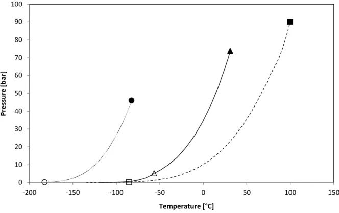
The vapor pressure is the basis of all equilibrium calculation. The vapor pressure curves for the three molecules of interest are shown in Fig. 6.

31

Fig. 6: Vapor pressure of the main components present in biogas

(■) H2S critical point ; (▲) CO2 critical point ; (●) CH4 critical point ; (□) H2S triple point ; (Δ) CO2 triple point ; (○) CH4 triple

point ; (- - - -) H2S ; (____) CO2 ; (……) CH4

The vapor pressures are calculated using Antoine Equation (2). The carbon dioxide vapor pressures above -76.36 °C were retrieved from the works of Kidnay [22], Yarym-Agaev [23], Miller [24] and Del Rio [25]. As shown in Fig. 6, the vapor pressure curve of CO2 continues at temperatures lower than the

triple point temperature (-56.56 °C) where it passes from Vapor – Liquid Equilibrium to Vapor – Solid Equilibrium.

log 𝑃 = 𝐴 − ( 𝐵

𝑇 + 𝐶) (2)

Where:

P [bar]: Vapor pressure. T [K]: Temperature.

A, B and C [-]: Component specific constants.

The constants used by Antoine Equation (2) are listed in Table 9 for each component.

Table 9. Constants used by Antoine Equation for the calculation of H2S, CO2 and CH4 vapor pressures

Components A B C Temperature range [K] References

H2S 4.43681 829.439 -25.412 138.8 – 212.8 [26] H2S 4.52887 958.587 -0.539 212.8 – 349.5 [26] CO2 6.81228 1301.679 -3.494 154.26 – 195.89 [27] CH4 3.9895 443.028 -0.49 90.99 – 189.99 [28] 0 10 20 30 40 50 60 70 80 90 100 -200 -150 -100 -50 0 50 100 150 Pr e ssur e [ b ar ] Temperature [°C]

32

2.3. Thermodynamic properties of the gas mixture (biogas)

2.3.1. Phase equilibrium behavior of biogas

In this section, the gas mixture is assumed to consist of methane (1) and carbon dioxide (2) because all the other impurities are present at very low concentrations depending on the type of substrate as shown in Table 4. Further, the upgrading process is generally made after purification that consists in the elimination of all these pollutants such as H2S, H2O and siloxanes.

The liquefaction of biomethane requires very low temperatures, therefore a cryogenic technology for biogas upgrading could be envisaged. This technology requires correct design of heat exchangers to achieve maximal purity of biomethane, that’s why the knowledge of the pressure – temperature behavior of the binary mixture methane – carbon dioxide is essential [29].

Fig. 7 presents the phase equilibrium behavior for the methane – carbon dioxide system.

Fig. 7: Pressure – Temperature equilibrium behavior for the CH4 – CO2 system [29]

(■) CH4 triple point ; (●) CH4 critical point ; (□) CO2 triple point ; (○) CO2 critical point ; (▲) mixture quadruple point ; (– –)

vapor-liquid critical locus ; (---) three-phase loci ; (—) pure compound phase equilibria

In the context of CO2 separation by solidification of CO2, the authors [29] have focused on the solid

phase because thanks to the high triple point of carbon dioxyde as seen in Table 7, CO2 could be

separated from methane directly from its gaseous phase into a solid phase for pressures close to the atmospheric pressure.

In order to understand the phase equilibrium behavior of the system CH4 (1) – H2S (2), Langè et al.

[30] have studied this aspect for temperatures from 70 K up to the critical tempearture of H2S and

33

Fig. 8: Pressure – Temperature equilibrium behavior for the CH4 – H2S system [30]

(─) three-phase equilibrium boundaries ; (∙∙∙) critical curves ; (– –) SVE, VLE and SLE of CH4 and H2S ; (■) quadruple point

34

2.3.2. Density and dynamic viscosity of biogas

All the thermophysical properties discussed in this section are calculated using the software REFPROP V9.0 which calculates the thermodynamic and transport properties of industrially important fluids and their mixtures. The equation of state for calculating these properties is the GERG (European Gas Research Group) – 2008 equation [31].

Depending on its composition, biogas has characteristics that it is interesting to investigate such as density and viscosity.

At a pressure of 1,103 bar, slightly higher than the atmospheric pressure, the variation of density as a function of temperature is shown in Fig. 9.

Fig. 9: Biogas density as a function of temperature

(____) Air ; (……) Biogas with 40 mol% of CO2 ; (- - - -) Biogas with 35 mol% of CO2

As seen in Fig. 9, biogas is lighter than air. Moreover, its density depends on the carbon dioxide content. The density of a biogas rich on carbon dioxide will be greater than that of a biogas containing an inferior CO2 concentration. This is due to the molecular weight of CO2 which is greater than that of

methane as seen in Tables 7 and 8.

At a pressure of 1,103 bar, the evolution of the viscosity of the biogas as a function of temperature is depicted in Fig. 10. 1 1.1 1.2 1.3 1.4 1.5 1.6 -30 -20 -10 0 10 20 30 40 50 60 D e n si ty [kg/m 3] Temperature [°C]

35

Fig. 10: Biogas viscosity as a function of temperature

(____) Air ; (……) Biogas with 40 mol% of CO2 ; (- - - -) Biogas with 35 mol% of CO2

As density, the biogas viscosity increases with the CO2 concentration. This is due to the higher

viscosity of carbon dioxide compared to methane, at equal pressure and temperature as shown in Tables 7 and 8.

2.3.3. Thermal conductivity of biogas

The thermal conductivity is a physical property which describes the ability of gases to conduct heat. The phenomenon of heat conduction in gases is explained by the kinetic gas theory which treats the collisions between the molecules.

The thermal conductivity depends on thermal capacity at constant volume and viscosity [32].

At a pressure of 1,103 bar, the variation of thermal conductivity of biogas as a function of temperature is shown in Fig. 11. 1.0E-05 1.2E-05 1.4E-05 1.6E-05 1.8E-05 2.0E-05 2.2E-05 -30 -20 -10 0 10 20 30 40 50 60 Vi sco si ty [Pa. s] Temperature [°C]

36

Fig. 11: Thermal conductivity of biogas as a function of temperature

(____) Air ; (……) Biogas with 40 mol% of CO2 ; (- - - -) Biogas with 35 mol% of CO2

As shown in Fig. 11, the thermal conductivity increases with temperature. This is due to collisions between the molecules of biogas that increase with temperature, resulting a thermal energy transfer increase.

2.3.4. Thermal capacities

The constant pressure heat capacity and the constant volume heat capacity are respectively related by the following thermodynamic Equations (3) and (4).

𝐶_𝑃= (𝜕𝐻

𝜕𝑇)_𝑃 (3)

𝐶_𝑉= (𝜕𝑈

𝜕𝑇)_𝑉 (4)

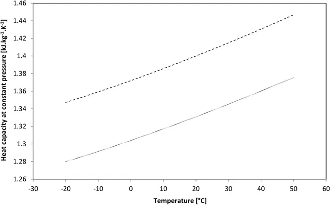
At a pressure of 1,103 bar, the variations of heat capacities of biogas as a function of temperature are shown in Fig. 12 and 13.

20 22 24 26 28 30 -30 -20 -10 0 10 20 30 40 50 60 Th e rm al c o n d u ctiv ity [m W. m -1.K -1] Temperature [°C]

37

Fig. 12: Heat capacity at constant pressure of biogas as a function of temperature

(……) Biogas with 60 mol% of CH4 ; (- - - -) Biogas with 65 mol% of CH4

Fig. 13: Heat capacity at constant volume of biogas as a function of temperature (……) Biogas with 60 mol% of CH4 ; (- - - -) Biogas with 65 mol% of CH4

Fig. 12 and 13 show that biogas specific heat capacities strongly depend on the methane concentration unlike the density, which is inversely proportional to the concentration of methane in the biogas. 1.26 1.28 1.3 1.32 1.34 1.36 1.38 1.4 1.42 1.44 1.46 -30 -20 -10 0 10 20 30 40 50 60 H e at cap ac ity at co n stan t p re ssur e [kJ .kg -1.K -1] Temperature [°C] 0.96 0.98 1 1.02 1.04 1.06 1.08 1.1 1.12 1.14 -30 -20 -10 0 10 20 30 40 50 60 H e at cap ac ity at co n stan t vo lu m e [ kJ .kg -1.K -1] Temperature [°C]

38

According to Vardanjan et al. [33], an increase of methane concentration from 50 % to 75 % will result in the increase of heat capacity by 17 %. In Fig. 12 and 13, heat capacities increased by 5 % after the passage of the methane concentration from 60 to 65 %.

2.4. Energy content in biogas

An important property of biogas is the lower heating value (LHV) which measures its energy value. The LHV of biogas is proportional to its methane content. For example, a biogas containing 70 mol% of methane at 15 °C and at atmospheric pressure has a LHV equal to 6.6 kWh/m3 _[34].

The energy value of biogas can also be evaluated by the Wobbe Index. Compared to the calorific value of biogas which has been treated by a lot of authors, only few studies have been conducted on the Wobbe index of biogas.

According to the Danish Technological Institute (DTI) [35], a biogas containing 60 mol% of methane, 38 mol% of carbon dioxide and 2 mol% of others has a Wobbe index of 19.5 MJ/m3_.

2.5. Conclusion

This chapter has allowed identifying the thermophysical properties of biogas. These properties are essential to design and optimize technologies for biogas purification and upgrading.

The thermophysical properties of biogas discussed in this chapter strongly depend on the composition of biogas, especially the concentrations of methane and carbon dioxide.

The presence of minor compounds such as H2O, N2, O2 and H2S could change the physical properties

of biogas. For example, landfill gas includes small amounts of nitrogen and oxygen which affect the phase behavior of the CH4 – CO2 system.

The technologies used for purification and upgrading of biogas will be discussed in the following section and a particular attention will be paid to the elimination of hydrogen sulfide.