Université Paris-Dauphine
Centre de Recherche en Mathématiques de la Décision UMR CNRS 7534
Regime Switching in Bond Yield and Spread
Dynamics
Changements de régimes dans la dynamique des taux et écarts de
taux obligataires
Thèse présentée et soutenue publiquement le
22 avril 2013
en vue de l’obtention du
Doctorat en Siences; discipline: Mathématiques Appliquées
par
Jean-Paul RENNE
Directeur de Recherche : Monsieur Alain MONFORT
Professeur des Universités
CREST, Banque de France, Université de Maastricht Rapporteurs : Monsieur René GARCIA
Professeur des Universités EDHEC Business School
Monsieur Patrick GAGLIARDINI
Professeur des Universités
Université de Lugano, Swiss Finance Institute Suffragants : Monsieur Christian GOURIÉROUX
Professeur des Universités
CREST, Université Paris-Dauphine, Université de Toronto
Monsieur Serge DAROLLES
Professeur associé
Université de Paris-Dauphine, QuantValley
Monsieur Christophe PÉRIGNON
Professeur de Finance HEC Paris
L’Université Paris-Dauphine n’entend donner aucune approbation ni improbation aux opinions émises dans les thèses; ces opinions doivent être considérées comme
.
Remerciements
En premier lieu, je tiens à adresser mes plus chaleureux remerciements à Alain Monfort, mon directeur de thèse. Il m’a transmis la passion de la recherche et n’a eu de cesse de m’encourager et de me soutenir pendant ces quatre années. C’est un honneur et un plaisir toujours grandissant de travailler avec lui.
Je remercie très sincèrement René Garcia et Patrick Gagliardini d’avoir accepté d’être rapporteurs de ma thèse. Je suis en outre honoré que Chritian Gouriéroux, Serge Darolles et Christophe Pérignon aient accepté de faire partie de mon jury. Je suis particulièrement reconnaissant envers Jean-Stéphane Mésonnier pour son soutien amical sans faille. Je remercie également Laurent Clerc et Benoît Mojon pour leur contribution à la faisabilité de ce projet.
Ce travail a bénéficié de nombreuses, sympathiques et fructueuses interactions avec mes collègues de la Banque de France.
Enfin, je souhaite remercier ma famille et ma belle-famille pour leur soutien, leurs questions et leurs encouragements. Je dédie ce travail à Marie, mon épouse, ainsi qu’à Marceau et Émile, mes enfants, grâce à qui chaque jour est une tranche de bonheur.
Contents
Abstract 8
1. Survey of the literature 11
1.1. Regime switching: A tool to model non-linear dynamics . . . 13
1.2. Regime switching in economics and finance . . . 14
1.3. Yield-curve dynamics and regime switching . . . 16
1.3.1. Regime shifts in default-free yield-curve dynamics . . . 16
1.3.2. Regime shifts in spreads’ dynamics . . . 17
1.4. Jointly modelling the physical and risk-neutral dynamics of different yield curves . . . 19
1.5. Systemic risk, default clustering and contagion . . . 21
1.6. Credit-migration modelling . . . 23
1.7. Monetary-policy and the yield curve . . . 25
1.8. Decomposing the term structure of spreads . . . 27
2. Default, liquidity and crises: An econometric framework 30 2.1. Introduction . . . 34
2.2. Information and historical dynamics . . . 37
2.2.1. Information . . . 37
2.2.2. Historical dynamics . . . 37
2.3. Stochastic discount factor and risk-neutral dynamics . . . 40
2.3.1. Stochastic discount factor . . . 40
2.3.2. Risk-neutral dynamics . . . 41
2.4. Pricing . . . 44
2.4.1. Defaultable bond pricing with zero recovery rate . . . 44
Contents
2.5. Internal consistency (IC) conditions . . . 47
2.5.1. IC conditions based on riskless yields . . . 47
2.5.2. IC conditions based on defaultable yields . . . 48
2.5.3. IC conditions based on asset returns . . . 48
2.6. Inference . . . 49
2.6.1. Observability . . . 49
2.6.2. Estimation methods . . . 49
2.6.3. Estimation example: a simple model of the BBB-Treasury spreads . . . 50
2.7. Liquidity risk . . . 55
2.8. Model extensions . . . 57
2.8.1. Multi-lag dynamics for yt and xn,t processes . . . 57
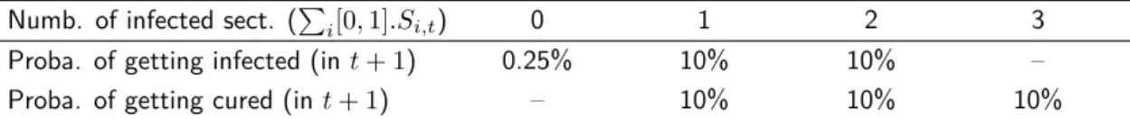
2.8.2. Interpretation of a regime as the default state of an entity . 58 2.8.3. A sector-contagion model . . . 60
2.8.4. modelling credit-rating transitions . . . 62
2.9. Conclusion . . . 67
2.A. Proofs of Sections 2.3 and 2.4 . . . 68
2.A.1. Proof of Proposition 1 . . . 68
2.A.2. Proof of Proposition 2 . . . 68
2.A.3. Pdf under the Q world . . . 69
2.A.4. The risk-neutral Laplace transform of (zt, yt, xn,t) . . . 69
2.A.5. Multi-horizon Laplace transform of a Car(1) process . . . 70
2.B. Kitagawa-Hamilton algorithm for partially-hidden Markov chains . 71 2.C. Inversion techniques in the presence of unobserved regimes . . . 73
2.C.1. Decomposition of the joint p.d.f. and estimation strategy . . 73
2.C.2. Estimation of the parameters (θzy, θ∗) . . . 74
2.C.3. Estimation of �θx n, θdn � . . . 76
2.D. Estimation example: U.S. BBB-AAA corporate spreads . . . 77
2.D.1. State-space model . . . 77
2.D.2. Estimation results . . . 78
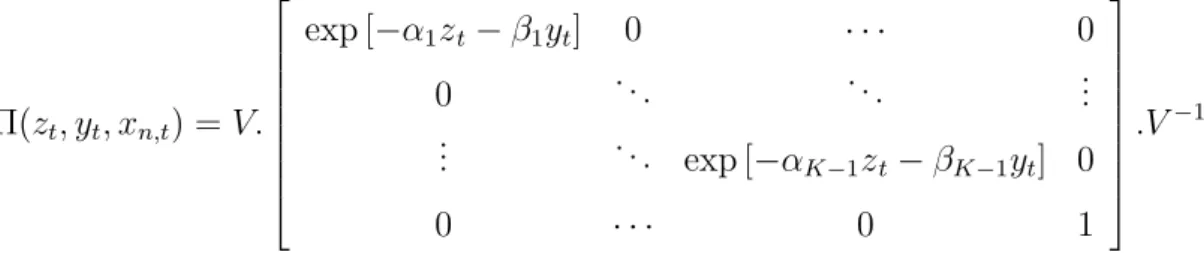
2.E. About the eigenvectors of the rating-migration matrix Π . . . 80
3. Credit and liquidity risks in euro-area sovereign yield curves 84 3.1. Introduction . . . 88
Contents
3.2. The model . . . 91
3.2.1. Historical dynamics of factors (yt) and regimes (zt) . . . 91
3.2.2. The risk-neutral dynamics . . . 93
3.2.3. Hazard rates . . . 93
3.2.4. Pricing . . . 94
3.3. Data . . . 96
3.3.1. The KfW-Bund spread . . . 96
3.3.2. Euro-area government yields . . . 97
3.3.3. Construction of the factors yt . . . 98
3.4. Estimation . . . 101
3.4.1. Main lines of the estimation strategy . . . 101
3.4.2. Historical dynamics of (zt, yt) . . . 101
3.4.3. Risk-neutral dynamics . . . 103
3.5. Results and interpretation . . . 106
3.5.1. The illiquidity intensity . . . 106
3.6. Conclusion . . . 110
3.A. Proofs . . . 111
3.A.1. Laplace transform of (zt, yt) . . . 111
3.B. Sovereign yield data . . . 112
3.C. Computation of the covariance matrix of the parameter estimates . 114 3.D. Disentangling credit from liquidity risks: the loss function . . . 116
4. Credit and liquidity pricing within the financial crisis 124 4.1. Introduction . . . 128
4.2. The model . . . 130
4.2.1. Default events, liquidity shocks and associated intensities . . 130
4.2.2. Historical dynamics of wt. . . 132
4.2.3. Stochastic discount factor and risk-neutral (Q) dynamics . . 135
4.2.4. Bond pricing . . . 136
4.3. Data . . . 137
4.3.1. Overview . . . 137
4.3.2. Euro-area government yields . . . 138
4.4. Estimation . . . 140
Contents
4.4.2. Estimation procedure and results . . . 141
4.5. Interpretation . . . 145
4.5.1. Credit and liquidity crises . . . 145
4.5.2. Liquidity intensity and pricing . . . 147
4.5.3. Default probabilities . . . 149
4.6. Conclusion . . . 151
4.A. Pricing of defaultable bonds . . . 152
4.B. Parameter constraints . . . 153
4.B.1. Econometric identification of the liquidity factor λ�,t . . . 153
4.B.2. Specification of the matrix of transition probabilities Π . . . 154
4.B.3. The size of the Gaussian shocks . . . 154
4.B.4. The auto-regressive coefficient ρc . . . 155
4.B.5. The standard deviations of the pricing errors . . . 156
4.C. Relationship between the risk-neutral and historical intensities . . . 156
5. A model of the euro-area yield curve with discrete policy rates 164 5.1. Introduction . . . 169
5.2. Data and stylised facts . . . 174
5.2.1. The EONIA and the Eurosystem’s framework . . . 174
5.2.2. The Overnight Index Swaps . . . 176
5.2.3. Data sources and treatments . . . 178
5.2.4. Preliminary analysis of the yields . . . 179
5.3. The model . . . 180
5.3.1. The components of the overnight interest rate . . . 180
5.3.2. Pricing . . . 186
5.4. Estimation . . . 188
5.4.1. The state-space form of the model . . . 188
5.4.2. Computation of the log-likelihood . . . 189
5.4.3. Estimation results . . . 190
5.5. Term premia associated with target changes . . . 193
5.6. Estimated impact of forward policy guidance . . . 195
5.7. Conclusion . . . 196
Contents
5.B. Multi-horizon Laplace transform of a (homogenous) Markov-switching
process . . . 199
5.C. Pricing formulas . . . 200
5.C.1. Computation of P1(t, h) . . . 201
5.C.2. Computation of P2(t, h) . . . 202
5.C.3. Computation of P3(t, h) . . . 203
5.D. Computation of the likelihood . . . 205
Bibliography 215
List of Figures
2.1. Causality scheme . . . 39
2.2. BBB vs. Treasury Spreads, Estimation results . . . 54
2.3. BBB vs. Treasury Spreads, Simulations . . . 81
2.4. Simulated sample of the sector-contagion model . . . 82
2.5. Yield curves for selected ratings (with impact of regimes) . 82 2.6. Simulated downgrade probabilities and spreads . . . 83
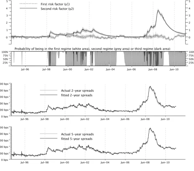
3.1. Differentials between government and government-guaranteed bonds . . . 98
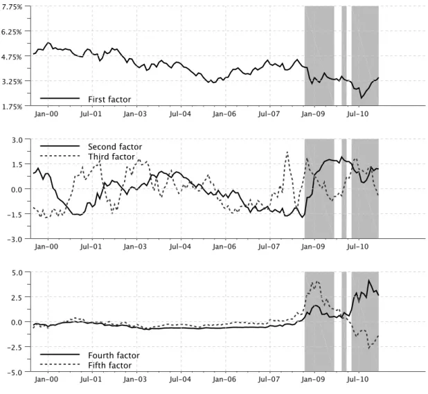
3.2. The five factors yt and the estimated regime variable zt 103 3.3. Model-based vs. survey-based forecasts . . . 104
3.4. Actual vs. model-implied spreads vs. Germany . . . 107
3.6. Sensitivity to the liquidity factor versus debt outstanding . . . 109
3.5. Liquidity intensity λ� t and liquidity-pricing proxies . . 123
4.1. Actual vs. model-implied spreads . . . 146
4.2. Estimated regimes and intensities . . . 159
4.3. Sensitivity to the liquidity factor versus debt outstanding . . . 160
4.4. Default probabilities estimates (5-year horizon) . . . 161
4.5. Term structure of default probabilities . . . 162
4.6. Default probabilities estimates (5-year horizon) . . . 163
5.1. Target rate, EONIA and OIS . . . 176
5.2. Estimated st process and model fit . . . 191
List of Figures
5.4. Changes in monetary-policy regimes and central-bankers’ announce-ments . . . 209 5.5. Fitted yield curves and influence of monetary-policy regimes
. . . 209 5.6. Estimated probabilities of regime changes . . . 210 5.7. Standard deviations associated with the 3-month-ahead forecasts of the
policy rate . . . 211 5.8. Risk-neutral vs. physical policy-rate forecasts, and associated risk premia
. . . 213 5.9. Simulation of forward-guidance measures . . . 214
List of Tables
2.1. Estimation methods . . . 50
2.2. Calibration of the sector-contagion model . . . 62
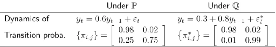
2.3. Dynamics of risk factors under both measures . . . 66
2.4. Baseline matrix of rating-migration probabilities . . . 66
2.5. Eigenvalues of the transition matrix under both regimes . . . 66
3.1. Descriptive statistics of selected yields . . . 99
3.2. Correlations and preliminary analysis of euro-area yield differentials . . . 119
3.3. Parameters defining the historical and risk-neutral dynamics (Part 1/2) . . . 120
3.4. Parameters defining the historical and risk-neutral dynamics (part 2/2) . . . 121
3.5. Estimation of the hazard-rate (λn,t) parameterizations 122 4.1. Descriptive statistics of selected spreads . . . 139
4.3. Parameter estimates (1/2) . . . 143
4.4. Parameter estimates (2/2) . . . 144
4.5. Conditional probabilities of transition . . . 145
4.2. Principal component analysis of euro-area yield differentials . . . 158
5.1. Descriptive statistics of yields . . . 207
Résumé
Cette thèse développe des modèles de la structure par terme de taux d’intérêt –et des écarts de taux d’intérêt– dans lesquels les changements de régimes occu-pent une place centrale. On montre notamment que ce type de modélisation est particulièrement adapté pour rendre compte du comportement non-linéaire de ce type de variables financières. Ces modèles sont exploités afin de répondre à des questions clés pour les décideurs économiques et/ou les participants de marché, notamment: quels sont les effets de la crise financière récente sur la structure par terme des taux d’Etat ? Comment modéliser l’influence du risque systémique sur la courbe des taux ? Comment l’illiquidité d’une obligation ou le risque de défaut de son émetteur influencent la valorisation de ce titre ? Quelles sont les compen-sations demandées par les investisseurs pour supporter le risque de taux associé aux décisions de politique monétaire ?
Les modèles présentés sont fondés sur l’hypothèse d’absence d’opportunité d’arbitrage. Ce type d’approche a acquis une importance croissante pour les décideurs comme pour les participants de marché au cours de la dernière décennie. En effet, tout en permettant un ajustement fin des données, les modèles vérifiant cette hypothèse fournissent un cadre cohérent pour l’analyse des fluctuations des taux obligataires et des primes de risque qu’elles incluent.
Dans la spécification de nos modèles, une grande importance est accordée à la simplicité des formules de valorisation d’actifs. Ceci est crucial pour l’estimation des paramètres des modèles et pour faciliter l’inférence statistique. La simplicité des calculs repose sur l’utilisation des propriétés des processus composés
auto-regressifs (Car) pour obtenir des formules quasi-explicites de prix obligataires1.
Dans notre approche, les dynamiques physique et risque-neutre des processus sont explicites. Disposer de la dynamique historique rend notamment possibles les exercices de prévision et, de manière générale, est important pour les besoins de gestion des risques financiers (notamment pour le calcul des Values-at-Risk, VaR). Le premier chapitre est une revue de la littérature liée aux différents sujets étudiés dans cette thèse. Dans le deuxième chapitre, nous développons un cadre général de modélisation des fluctuations de courbes de taux associées à différents émetteurs. Les probabilités de défaut des emprunteurs sont fonctions de facteurs observables ou non, à valeurs discrètes ou réelles. Alors que l’accent est mis sur la modéli-sation du risque de défaut, on montre comment ce cadre permet également de valoriser les titres obligataires illiquides. Une version simple du modèle est es-timée pour reproduire la dynamique des écarts de taux entre les obligations émises par des entreprises américaines d’une part et celles émises par le Trésor américain (Treasuries) d’autre part. Ce second chapitre montre par ailleurs comment les changements de régimes peuvent être utilisés pour reproduire des phénomènes de contagion sectorielle. Enfin, le cadre initial est étendu pour modéliser les transi-tions de notatransi-tions de crédit et l’influence de celles-ci sur les structures par terme de taux d’intérêt.
Le chapitre 3 présente une analyse des fluctuations jointes de courbes de taux d’Etat de dix pays de la zone euro entre 1999 et 2012. Deux régimes intervi-ennent dans le modèle, l’un de ceux-ci correspondant aux périodes de crise fi-nancière. Ces régimes conditionnent la dynamique de cinq facteurs observables. Le taux d’intérêt sans risque de court-terme, ainsi que les intensités de défaut et d’illiquidité, dépendent linéairement de ces cinq facteurs. Ces spécifications permettent d’expliquer la majeure partie des variations des taux d’intérêt inclus dans l’échantillon –pour les différents pays et les différentes maturités considérées. L’estimation suggère en outre que l’introduction du régime de crise est importante pour expliquer l’accroissement de la volatilité des écarts de taux sur la période récente. Cette étude propose également un moyen d’identifier la partie des taux
d’intérêt liée à la valorisation de l’illiquidité relative des obligations souveraines. A cet égard, les résultats indiquent que bien que la liquidité soit un facteur im-portant pour expliquer les écarts de taux d’Etat sur les cinq dernières années, les inquiétudes relatives à la qualité de crédit des Etats de la zone euro constituent le principal motif de leurs variations sur la période 2010-2012.
Le chapitre 4 complète l’analyse du chapitre précédent en se concentrant sur les cinq dernières années, i.e. la période de crise financière 2007-2012. La modélisation repose sur des facteurs de risque latents (non observables). La modélisation des périodes de crise est plus précise que dans le chapitre précédent. En effet, nous distinguons ici deux types de tensions : celles liées à des motifs de liquidité et celles liées à des motifs de crédit. Plus précisément, nous introduisons deux chaînes, l’une dite de liquidité et l’autre dite de crédit. Pour la chaine de liquidité, deux états sont possibles: «faibles tensions» et «périodes de turbulences». Pour la chaîne de crédit, un troisième niveau de tension («crise aigue») s’ajoute aux deux premiers. L’estimation met en évidence un lien de causalité entre les deux types de tensions : la probabilité d’entrer dans une période de turbulences liées à des modifs de crédit est plus forte lorsque la situtation de liquidité est déjà détériorée.
Le chapitre 5 examine l’influence de la politique monétaire sur la courbe des taux d’intérêt. Bien que les taux directeurs fixés par la banque centrale jouent un rôle central dans la dynamique de la structure par terme des taux d’intérêt, peu de modèles sont cohérents avec les spécificités des trajectoires de taux directeurs. Ce chapitre vise à pallier ce manque en présentant un cadre dans lequel le taux d’intérêt (de court terme) auquel les banques se refinancent auprès de la banque centrale est à valeurs discrètes (ce sont des multiples de 0.25%) et positives. En particulier, contrairement à la plupart des modèles de la structure par terme, celui-ci est conforme à l’existence d’une borne inférieure (en zéro) pour les taux courts. Ces propriétés découlent d’une utilisation innovante (et intensive) des changements de régimes. En dépit d’un très grand nombre de régimes (246), le modèle reste maniable, ce qui est illustré par son estimation sur données quotidiennes relatives à la zone euro, l’échantillon couvrant les 13 dernières années. Les résultats suggèrent que la partie courte de la courbe des taux intègre des primes de risque, celles-ci
correspondant aux compensations demandées par les investisseurs pour supporter le risque de taux associé aux décisions de politique monétaire. Ce modèle est également utilisé afin d’évaluer l’influence sur la courbe des taux d’engagements de la banque centrale sur une trajectoire future de son principal taux directeur.
Summary
This doctoral thesis studies the potential of regime-switching models to capture salient features of the dynamics of interest rates. It is notably shown that these techniques can be used in several ways to reproduce various forms of yield and spread non-linearities. Different innovative frameworks, combining flexibility and tractability, are proposed. They are brought to data so as to tackle questions that are key for both policy-makers and practitioners alike. These questions include the following: What are the effects of the ongoing financial crisis on the term-structure of sovereign spreads? How to model yield-curve reactions to increases in systemic risk? What are the effects of market liquidity on the term structure of interest rates? How are priced the probabilities of default (PDs) in defaultable-bond yields of different maturities? What are the compensations required by investors to hedge against uncertain monetary-policy decisions?
The models that are presented throughout this thesis rule out arbitrage oppor-tunities. Such models are becoming increasingly important to policy makers and practitioners. Indeed, beyond being able to provide a good fit of interest rates along the whole maturity spectrum, these models allow to study the driving factors be-hind the term structure of interest rates and the risk premia within a consistent framework.
Particular attention is paid to the tractability of the proposed models. Tractability is notably obtained through an extensive use of Car’s –Compound autoregressive processes– properties,2which leads to quasi-explicit formulas for bond prices. Both
historical and risk-neutral dynamics are explicitly modeled, which is helpful for
choosing appropriate specifications under the physical –or real-world– measure, for dealing simultaneously with pricing and forecasting or also for risk-management purposes (e.g. Value-at-Risk calculations).
The first chapter of this dissertation goes through the different topics that are studied in the thesis and reviews the connected literature. The second chapter develops a general framework aimed at modelling the joint dynamics of yield curves associated with different issuers. In this reduced-form framework, the default probabilities are modeled directly as functions of observable or latent factors, the latter being discrete or real-valued. Regime-switching features lie at the heart of this framework. While the focus is on default modelling, the specifications can also account for the pricing of some liquidity premia using the same machinery (as in Duffie and Singleton, 1999). A basic form of the model is fitted on the term structure of spreads between U.S. corporate BBB-rated bonds and risk-free (Treasury) yields. Some extensions are proposed, including a sector-contagion model as well as the explicit modelling of credit-rating transitions.
In Chapter 3, the framework is applied to model the joint fluctuations of ten euro-area sovereign yield curves over the period 1999-2012. In the model, there are two regimes: a “tranquil” regime and a crisis one. These regimes affect the dynamics of five euro-area wide observable factors. These factors affect the riskfree short-term rate as well as the default and illiquidity intensities associated with the different issuers. This framework is able to capture most of the fluctuations of the various interest rates (over the different countries and different maturities) of the estimation sample. Further, the setup makes it possible to account for the dramatic rise in spreads that have been observed for some countries over the last few years. Also, this study proposes a way to identify liquidity-related components in sovereign bond yields. Regarding the latter point, the estimation results suggest that while liquidity is an important driver of euro-area sovereign spreads, most of the 2010-2012 spreads’ fluctuations correspond to concerns regarding the credit quality of sovereign issuers.
of the last thirteen years hereinbefore). Contrary to Chapter 3, the pricing factors are unobservable. In addition, the crisis modelling is more precise. Specifically, we distinguish between two kinds of crises: liquidity-related ones and credit-related ones. For the credit chain, there are three possible states: “calmer periods”, “turmoil periods” and “severe-crisis periods”; for the liquidity chain, there are two possible states: “calmer periods” and “turmoil periods”. The empirical part of Chapter 4 provides evidence of causality between the two types of crisis, the probability of switching from the calm credit state to the credit-crisis state being higher when the liquidity situation is already deteriorated.
Chapter 5 investigates the influence of monetary policy on the yield curve. In this study, a key role is given to the central-bank policy rate. In the model, the policy rate follows a realistic step-like path (with values that are multiples of 0.25%) and can not turn negative. Therefore, by contrast with most of the existing term-structure models, this one is consistent with the zero-lower bound (ZLB). These appealing features are obtained thanks to an extensive and innovative use of regime shifts. In spite of a very large number of regimes (246), the model remains tractable and is easily brought to data. This is illustrated by estimating the model on euro-area daily data covering the last 13 years. The results notably point to the existence of monetary-policy-related risk premia at the short-end of the yield curve. Furthermore, this model is used in order to assess the influence of forward-guidance measures –defined as commitments of the central bank regarding the future paths of the policy rate– on the yield curve.
1. Survey of the literature
Abstract: This first chapter reviews the literature connected to the present thesis.
Section 1.1 surveys the contributions that have highlighted the ability of Marko-vian regime-switching techniques to model nonlinear dynamics in a tractable way. Section 1.2 illustrates the fact that these techniques have been employed in many studies exploring the dynamics of economic and financial variables. Section 1.3 focuses on the use of regime switching in term-structure models: Subsection 1.3.1 deals with risk-free yields and Subsection 1.3.2 considers defaultable-bond pricing. The subsequent Sections deal with the additional topics that are covered by this thesis: the simultaneous modelling of different yield curves (Section 1.4), systemic risk and contagion (Section 1.5), credit-rating migrations (Section 1.6), monetary-policy and the yield curve (Section 1.7) and the decomposition in spreads into liquidity and credit components (Section 1.8).
Survey of the literature
Résumé
Il existe une importante littérature sur l’existence de non-linéarités dans la dy-namique des taux d’intérêt (voir par exemple Aït-Sahalia, 1996, Stanton, 1997 ou Boudoukh et al., 1999). Plus précisément, plusieurs études montrent l’existence de différents régimes conditionnant la dynamique des taux d’intérêt (voir notamment Hamilton, 1988 ou Ang et Bekaert, 2002).
Alors que le comportement récent des taux d’intérêt illustre de manière édifiante la notion de changement de régimes, l’utilisation de modèles à changements de régimes pour l’analyse de la structure par terme des taux d’intérêt est encore relativement limitée. Alors que différentes études présentent des modèles dans lesquels les déformations d’une unique courbe de taux dépendent de l’état d’une variable aléatoire à valeurs discrètes (Monfort et Pégoraro, 2007, Ang, Bekaert et Wei, 2008, Dai, Singleton et Yang, 2007, ou Pérignon and Smith, 2007), un nombre très restreint de contributions considèrent la modélisation jointe de différentes courbes de taux affectées par des changements de régimes (Dionne et al., 2011 et Siu, Erlwein et Mamon, 2008).
Ce premier chapitre propose une revue de la littérature concernant la modélisation des changements de régimes d’une manière générale et leurs applications à la mod-élisation des variables financières et des taux d’intérêt en particulier. Cette revue de la littérature couvre également divers champs d’études auxquels les travaux présentés dans cette thèse sont liés, ceux-ci ont trait à:
• la modélisation du risque systémique et des phénomènes de contagion; • la modélisation des changements de notations de crédit;
• l’influence de la politique monétaire sur la structure par terme des taux d’intérêt;
• l’influence de la valorisation de la qualité de crédit et de la liquidité sur la structure par terme des taux d’intérêt.
1.1 Regime switching: A tool to model non-linear dynamics
1.1. Regime switching: A tool to model non-linear
dynamics
Linear models –such as autoregressive (AR) models, moving average (MA) models, and mixed ARMA models– are extensively used to model the dynamics of economic or financial variables. These models, that are extremely popular among academics, practitioners and policy makers, are quite successful in numerous applications. However, it has often been found that simple linear time series models usually leave certain aspects of economic and financial data unexplained. By definition, they are unable to capture nonlinear dynamic patterns such as asymmetry, extreme events or volatility clustering. Typically, the properties of output growth in recessions are, in various ways, different from expansion time (see e.g. Hamilton, 1989, Lo and Piger, 2005 or Sichel, 1994 among innumerable others). Inflation also presents different kinds of nonlinearities, notably in crises periods (see e.g. Stock and Watson, 2010). Therefore, in many cases, linear models are not sufficient and non-linear approaches have to be resorted to. Accordingly, over the last two to three decades, we have witnessed a rapid growth of the development of nonlinear time series models (see e.g. Granger and Te¨rasvirta, 1993).
Regime-switching models, closely linked to the seminal work of Hamilton (1988, 1989 and 1990), are among the most popular nonlinear time series models in the literature. The fact that the regimes can switch over time makes it possible to account for various non-linear behavior of the modeled variables. In the standard regime-switching framework, the change in the regimes is controlled by an un-observable state variable that follows a Markov chain, that is, the current value of the state variable depends on its immediate past value. A given regime can be persistent or not, depending on the probabilities of switching to alternative regimes. The Markov switching model is therefore suitable for describing corre-lated data that exhibit distinct dynamic patterns during different time periods. The standard framework has notably been extended by Filardo (1994) to allow for time-varying transition probabilities (implying that regime-switching models encompass threshold auto-regressive models of Tong and Lim, 1980) or, from an
1.2 Regime switching in economics and finance
econometric point of view, by Kim (1994) that integrates the regime-switching features within a state-space framework including unobserved factors affected by Gaussian shocks.
Of course, regime-switching models are not the only models that can handle non-linear behavior of random variables. There exist models that can handle more general forms of non-linearity. In particular, the so-called artificial neural network models, due to their “universal approximation” property, are capable of charac-terizing any nonlinear pattern in data (see e.g. Kuan and White, 1994). Un-fortunately, these models suffer from identification-related problems and are far less tractable than regime-switching models. As will be illustrated throughout the present thesis, the latter still allow for a substantial degree of flexibility, making them appropriate to study a wide range of phenomena.
By appropriately mixing conditional normal (or other types of) distributions, large amounts of non-linear effects can be generated within regime-switching frame-works. Regime switching models can provide a good approximation for more com-plicated processes driving security returns. Regime switching models also nest as a special case jump models, since a jump is a regime which is immediately exited next period and, when the number of regimes is large, the dynamics of a regime switch-ing model approximates the behavior of time-varyswitch-ing parameter models where the continuous state space of the parameter is appropriately discretized.
1.2. Regime switching in economics and finance
Abrupt changes are a prevalent feature of economic systems and financial markets. These changes are of different natures: some are transitory (jump-like) and some tend to persist for protracted periods. As mentioned above, both types of changes can be captured by regime-switching models (see Ang and Timmermann, 2011 and Guidolin, 2011); this is going to be illustrated in the present thesis.1
Regime-switching models parsimoniously capture stylized behavior of many financial series
1Specifically, in the model developed in Chapter 3, the crisis regime may last for several years.
1.2 Regime switching in economics and finance
including asymmetries, fat tails, skewness, persistently occurring periods of tur-bulence followed by periods of low volatility, volatility clustering, time-varying correlations.
The use of the regime-switching method for modelling dynamics and asymmetries in stock prices has become very popular and various adaptations of the basic set-up have been proposed (e.g. Perez-Quiros and Timmermann, 2001 or Ang and Chen, 2002). Regime-switching setups have also been estimated to analyze the dynamics of exchange rates (Ang, 2011, Kanas, 2006, Engel, 1994, Bollen, Gray and Whaley, 2000 and Dewachter, 2001), and of various alternative prices such as electricity prices (e.g. Haldrup and Nielsen, 2006) or commodity prices (e.g. Chen and Insley, 2012).
Regime-switching models have proven useful in building coincident indicators (Kim and Yoo, 1995 and Kim and Nelson, 1998) or in developing forecasting tools (Chau-vet and Potter, 2000) or optimal portfolio choice (Guidolin and Timmermann, 2007).
The ongoing financial crisis is strengthening the case for including regime-switching features in financial models (see Christensen, Lopez and Rudebusch, 2008). This is notably illustrated by Chapters 3 and 4 of the present thesis that study the dynamics of government-bond interest rates amid the so-called euro-area sovereign debt crisis (exploiting the general framework presented in Chapter 2). The crisis period itself can be seen as a succession of different regimes or phases; this idea is omnipresent: it can be found in academic work (e.g. Bech and Lengwiler, 2011), in official speeches (Stark, 2009) or in the medias (The Guardian, 2011).
The fact that the idea of regime changes is natural and intuitive has contributed to its popularity. Economic explanations for these types of time-variation in a series’ dynamics point into main three directions. According to the first, regimes identified by econometric methods can be associated with different periods in reg-ulation, policy, and other secular changes (see e.g. Hamilton, 1988, Sims and Zha, 2006, Davig, 2004). The second strand of economic explanations relates market-price movements to macroeconomic fundamental influences. In particular,
1.3 Yield-curve dynamics and regime switching
numerous studies confirm that the conditional moments of stock returns are busi-ness cycle dependent (Cecchetti, Lam and Mark, 1990, Hamilton and Lin, 1996, Schwert, 1989, Campbell et al., 2001 or Perez-Quiros and Timmermann, 2001). The third type of explanation attributes nonlinearities to particular behavior of market participants (e.g. noise traders). There is a large literature that reports that speculative trading may cause fads, bubbles or even market crashes (Funke, Hall and Sola, 1994, van Norden and Vigfusson, 1998 or Jeanne and Rose, 2002).
1.3. Yield-curve dynamics and regime switching
1.3.1. Regime shifts in default-free yield-curve dynamics
Strong evidence points to the existence of regime switching in the dynamics of the term structure of interest rates. Thus, Hamilton (1988) finds that changes in the Federal reserve operating procedures leads to regime-switching in the dynamics of the term structure of interest rates. In addition to such a shift, Cai (1994) finds that the 1974 oil shock resulted in a regime shift in the asymptotic volatility of the three-month Treasury bill. Gray (1996) shows that the assumption of a single regime is a source of misspecification in models of the short rate. Garcia and Perron (1996) use the Hamilton filter to characterize the time series behavior of the ex-post U.S. real interest rate during the period 1961 to 1986 and show that the real interest rate series during this time period would be best characterized by three states. Adding term spread in their estimation, Ang and Bekaert (2002) identify regimes that are closely linked to business cycles, suggesting that large periodic shifts in interest rates across distinct regimes present a systematic risk to investors (see also Wu and Zeng, 2005 or Bansal and Zhou, 2002). The same authors (2002) show that regime switching is efficient in capturing nonlinear dynamics of the short-term interest rate exhibited by Aït-Sahalia (1996). Christiansen (2004) estimates a two-state Markov-switching model for the short-rate and the slope of the yield curve: his estimated regimes turn out to depict low and high variances regimes for short-rate changes. The economy appears to have been in the high-variance
1.3 Yield-curve dynamics and regime switching
state during unusual economic periods such as oil or stock-market crises, or more generally during the official recession periods.
Monfort and Pegoraro (2007) show that the introduction of regime switching in term-structure models leads to term-structure models that are well-specified under the historical probability and that are able to explain the expectation-hypothesis puzzle (why the long and short term interest rate differential does not predict the future interest rate changes), over short and long horizons. Following Veronesi and Yared (1999) and Evans (2003), Ang Bekaert and Wei (2008) develop term structure models with regime shifts to investigate the joint dynamics of real and nominal yields. They identify inflation and real factor sources behind regime shifts and analyze how they contribute to nominal interest-rate variations. Dai, Singleton and Yang (2007) develop a model with regime-shift risks that are priced by investors. Allowing for state-dependent transition probabilities, their model makes it possible to conveniently capture asymmetry in the cyclical behavior of interest rates. Pérignon and Smith (2007) show that allowing for regime shifts in the pricing factor volatilities dramatically improves the model’s fit.
In Chapters 2 to 4 of the present thesis, the emphasis is put on defaultable-bond pricing. By contrast, in Chapter 5, an innovative use of regime-switching features is proposed to model the term structure of riskfree yields. Contrary to the above-mentioned studies, the number of regimes involved in the model introduced in Chapter 5 can be very large (tens or hundreds). In spite of that, the model remains tractable and makes it possible to model the specific dynamics of the central-bank policy rate in a satisfying way. The latter point implies that this model can be exploited to investigate the effects of monetary-policy on the yield curve.2
1.3.2. Regime shifts in spreads’ dynamics
While the previous subsection puts forward the importance of modelling regime switching in yield-curve models, a few has been done to integrate such a feature in term-structure models of defaultable bonds. However, empirical studies point
1.3 Yield-curve dynamics and regime switching
to the existence of different regimes in the default risk valuation. Davies (2004 and 2008) uses Markov-Switching Vector Auto-Regression (MS-VAR) estimation techniques and finds that credit spreads exhibit distinct high- and low-volatility regimes. Alexander and Kaeck (2008) detect a pronounced regime-specific be-havior of Credit default swap (CDS) spreads. Cenesizoglu and Essid (2010) or Bruche and Gonzales-Aquado (2010) find switching behavior in default rates and recovery-rate distributions. Hackbarth, Miao and Morellec (2006) build a theoret-ical model to explain the dependence of credit spread on business-cycle regimes. In the same vein, Bhamra, Kuehn and Strebulaev (2007), Chen (2008) and David (2008) adopt a Merton structural model including regime switching to assess the influence of different states of the economic cycles on the credit-risk premia. This can be related to the analysis of Bangia et al. (2002) who illustrate the importance of distinguishing between expansion and contraction phases for the assessment of loss distribution of credit portfolios. Without deriving a complete model of the credit-spread term structure, Maalaoui, Dionne and François (2009) estimate Markov-switching specifications to investigate the links between credit spreads and their determinants. Their results suggest that the failure of single-regime models to find significant links between potential determinants (see e.g. Collin-Dufresne, Goldstein and Martin, 2001) may stem from the fact that these determinants have opposite average effects in the two regimes they identify. Dionne et al. (2011) propose a model of the term-structure of interest rates associated with default-able bonds. Regime switching affects the dynamics of the risk factors, that are observable macroeconomic variables. Siu, Erlwein and Mamon (2008) present a framework to price credit default swaps in the presence of regime-switching in the default intensities processes.
The potential of regime-switching features to account for the fluctuations of the term-structure of (credit-)risky yields in a no-arbitrage framework is explored in Chapters 2 to 4 of this thesis. In the proposed setups, the probabilities of default of the debtors depend on the different regimes and on factors that can be observed or latent. Therefore, the whole term structure of interest rates is affected by the regimes. While this framework is highly flexible, it remains particularly tractable,
1.4 Jointly modelling the physical and risk-neutral dynamics of different yield curves
bond yields being given by quasi-explicit formula. This property stems from the fact that the processes involved are Compound auto-regressive (Car), implying that multi-horizon Laplace transforms of these processes are obtained by recursive formulas.
1.4. Jointly modelling the physical and risk-neutral
dynamics of different yield curves
Motivated by derivative-pricing or credit-risk-management objectives, a large strand of the recent literature related to fixed-income securities has focused on the joint modelling of several yield curves. In this context, Jarrow, Lando, Turnbull (1997), Lando (1998) or Duffie and Singleton (1999) have highlighted the potential of affine term-structure models (ATSM) to describe the joint dynamics of yield curves as-sociated with various obligors subject to default risk. Their intensity-based –or reduced-form– approaches used to model defaults differ from the more structural approaches originating in Black and Scholes (1973) and Merton (1974). In the latter, the default of a firm is modeled in terms of the relationship between its assets and liabilities. The asset value process is modeled as a geometric Brown-ian motion and default occurs when the asset value at maturity is lower than the liabilities. Important industry models like KMV’s Portfolio Manager or the JP Morgan’s CreditMetrics model are based on this approach (see Crouhy, Glai and Mark, 2000for a comparative analysis of industry credit-risk models). Cathcart and El-Jahel, 2006) have shown that the two approaches (reduced-form and struc-tural) are somewhat reconcilable. As shown by Duffie and Singleton (1999), in an intensity-based framework, the modelling of defaultable claims is based on the standard affine term-structure machinery readily available for default risk mod-elling and estimation. Since then, numerous further developments have illustrated the flexibility and tractability of affine-term structure models to jointly model dif-ferent yield curves (see e.g. Duffee, 1999, Collin-Dufresne and Solnik, 2001, Dai and Singleton, 2003, Collin-Dufresne, Goldstein and Hugonnier, 2004 and
Gourier-1.4 Jointly modelling the physical and risk-neutral dynamics of different yield curves
oux, Monfort and Polimenis, 2006).
Despite the importance of sovereign credit risk in the financial markets, relatively little research proposing models of the joint dynamics of sovereign yields has ap-peared in the literature. Notable recent exceptions include Pan and Singleton (2008) and Longstaff et al. (2011). These two contributions point to an important degree of commonality across sovereign credit risk. More precisely, they show that the risk premia included in sovereign credit spreads are substantial and covary im-portantly with economic measures of global event risk. According to Longstaff et al., an important source of commonality in sovereign credit spreads may be their sensitivity to the funding needs of major investors in the sovereign credit markets. Chapters 3 and 4 propose models that depict the joint dynamics of different euro-area sovereign yield curves. In these models, the dynamics of the stochastic dis-count factor implies that the physical and the risk-neutral dynamics of the pricing factors –and notably the default process– do not coincide. The risk-neutral dynam-ics is the dynamdynam-ics of the pricing factors that would be consistent with observed prices under the (potentially false) assumption that investors are risk-neutral. In our framework, we can assess the size of the (potential) errors that are implied by assuming that the historical and the risk-neutral dynamics coincide. A typical example lies in the computation of market-based probabilities of default (PDs). To get these, the vast majority of practitioners or market analysts resort to ap-proaches ending up with risk-neutral PDs.3 While risk-neutral PDs are relevant
for pricing purposes, historical ones are needed (a) if one wants to extract real-world investors’ perception of the credit quality of the issuer, (b) for the sake of forecasting or more generally (c) for risk management purposes.4
3Most of these methodologies build on Litterman and Iben (1991), see e.g. (amongst many
others) Bank of England (2012), CMA (2011) and O’Kane and Turnbull (2003). Studies resorting to these methods are usually silent about this caveat. Notable recent exceptions include Blundell-Wignall and Slovik (2010), in an OECD study, who note: “In the real world, actual defaults are fewer than market-driven default probability calculations would indicate. That is because market participants demand a risk premium – an excess return – compared to the risk-neutral rate, and that premium cannot be observed. This makes it difficult to use the above measure [the risk-neutral PDs] to imply the likelihood of actual defaults in the periphery of Europe or anywhere else.”
4Regarding the latter point, note for instance that Value-at-Risk measures (VaR) should be
1.5 Systemic risk, default clustering and contagion
The results of Chapters 3 and 4 suggest that the sources of common fluctuations across euro-area countries’ yields command such credit-risk premia. This is con-sistent with the fact that sovereign risk cannot be diversified away. The analysis shows that, because of these premia, the physical probabilities of default of euro-area countries are substantially lower than their risk-neutral counterparts.
1.5. Systemic risk, default clustering and contagion
While there is no strong consensus on the definition of systemic risk, the general view is that this kind of risk would differ from the systematic ones in terms of the severity and frequency of the associated shocks. More precisely, systematic shocks are frequent and not extreme while systemic shocks would be infrequent and extreme (see e.g. Das and Uppal, 2004 or Baur and Schulze, 2009). For de Bandt and Hartmann (2000), a systemic event is an event where the release of bad news about a financial institution, or even its failure, or the crash of a financial market leads in a sequential fashion to considerable adverse effects on one or sev-eral other financial institutions or markets, e.g. their failure or crash. Obviously, disentangling systematic from systemic risks may not be a trivial task. In partic-ular, difficulties arise from the fact that systematic shocks can turn into systemic ones. For instance, in some contexts –notably when the level of uncertainty is high–, temporary systematic shocks can lead to defaults and generate significant negative aftershocks, including liquidity spirals.5
In a model accommodating regime shifts, it is natural to associate systematic and systemic risk with the Gaussian shocks and the regime shifts, respectively (see e.g. Gonzales-Hermosillo and Hesse, 2009 or Abdymomunov, 2012). Billio et al. (2012) propose an other use of regime-switching features to investigate systemic risks; in their approach, the regimes are key to model of the interconnectedness of the financial system.
2009).
5See Brunnermeier and Pedersen, 2009 for a structural analysis of this and e.g. Hesse and
1.5 Systemic risk, default clustering and contagion
The contagion literature focuses on the interdependencies between the defaults of different debtors.6 In the so-called contagion models, if one of the debtor defaults,
it affects the default probability of the other debtors. Contagion effects, whose consequences are cascades of subsequent spread changes, are explained by the existence of close ties between firms. These ties may be of legal (e.g. parent-subsidiary), financial (e.g. trade credit), or business nature (e.g. buyer-supplier). Through these channels, economic distress of one firm can have an immediate adverse effect on the financial health of that firm’s business partners (Giesecke, 2004, Egloff, Leippold and Vanini, 2005). Jarrow and Yu (2001) develop a
primary-secondary approach: in case a primary entity defaults, the spreads of other debtors
jump upwards; meanwhile, default of secondary firms do not have any impact on other debtors in the portfolio. In the infectious-default model developed by Davies and Lo (2001), the default of a debtor triggers a regime shift: in the high-risk regime, the default intensities of all debtors are increased.7
Das et al. (2007) test whether default events can reasonably be modeled as depen-dent solely on exogenous observable factors.8 As Duffie et al. (2009) and Giesecke
and Kim (2010), they find that doubly-stochastic settings perform badly if no la-tent covariates –also called frailty components– enter the intensity specifications. Duffie et al. (2009) further argue that including frailty covariates in the hazard-rate specifications is necessary to accommodate default clustering.9 Collin-Dufresne,
Goldstein and Helwege (2008), Bai et al. (2012) and Jorion and Zhang (2007) also find that default events are associated with significant increases in the credit spreads of other firms, consistent with default clustering in excess of that sug-gested by the standard doubly stochastic models. Azizpour and Giesecke (2008) find that contagion effects represent a significant additional source of default
clus-6For an extensive survey of the contagion literature, see e.g. Lütkebohmert (2009).
7Other contagion mechanisms based on the same kinds of approaches are proposed by Frey and
Backhaus (2003) or Yu (2007).
8Nevertheless, using a different specification of the default intensity, Lando and Nielsen (2008)
cannot reject the assumption of conditional independence for default histories recorder by Moody’s between 1982 and 2006. Lando and Nielsen conclude that the test proposed by Das et al. (2007) is mainly a misspecification test.
9Frailty models come from the biostatistics literature. In these models, the intensity of a point
process is proportional to an unobservable variable, the frailty parameter. For a survey of frailty models, see Hougaard (2000) [155].
1.6 Credit-migration modelling
tering (over and beyond the effect due to firms’ exposure to observable and frailty risk factors). Koopman, Lucas and Schwaab (2012) show that modelling frailty contributes to obtain a proper modelling of default rates during crisis.
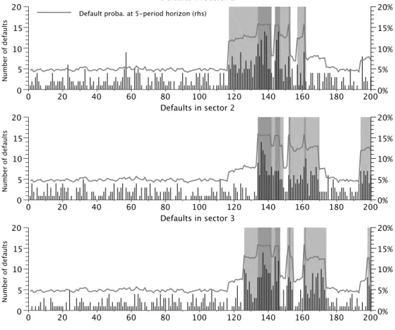
Two Subsections of Chapter 3 specifically deal with systemic risk and contagion. Subsection 2.8.2 shows that the general framework introduced in Chapter 3 can accommodate the specific contagion case where one entity –or, for the sake of tractability, a small number of them– affects the default probability of the others: it suffices to make one of the regimes corresponds to the default state of this entity. Further, Subsection 2.8.3 explains how the regime-switching feature can be exploited in order to capture “sector-contagion” phenomena. The sectors can represent different industries or different geographical areas. Each sector can be “infected” or not, and when a sector gets infected, the default intensities of its constituents (the debtors) shift upwards. In this context, sector contagion stems from the parameterization of the matrix of regime-transition probabilities. For instance, it is easy to model infection probabilities that depend positively on the number of sectors already infected.
1.6. Credit-migration modelling
The default of a debtor is the most basic credit event. More generally, credit events include changes in credit ratings like these attributed by agencies like Moody’s, Standard & Poor’s or Fitch. There are several reasons why it may be desirable to model not only default events but also rating transitions (see Cantor, 2004 or Gagliardini and Gourieroux, 2001). Several of the main credit models currently being used in the industry, such as J.P. Morgan’s CreditMetrics (1997), draw on the credit-migration approach. For presentation, comparison and evaluation of these models, one can refer to Crouhy, Glai and Mark (2000), Gordy (2000) or Lopez and Saidenberg (2000). First, because of the importance of ratings in terms of risk management, modelling credit migration is key for practitioners. For instance, the VaR or capital adequacy numbers may be based on a portfolio rating’s distribution (see Saidenberg and Schuermann, 2003). In addition, some portfolio
1.6 Credit-migration modelling
managers are constrained by limits based on the ratings of the bond they held. Second, such models are obviously required to price credit-event options. Third, when complete default historical data sets are not available (or do not go back far in time), exploiting credit-migration matrices may allow to extrapolate long-term default predictions from short-term credit risk dynamics. Similarly, to the extent that rating classes are seen as approximately homogenous, having a rating-based term structure model at one’s disposal makes it quick to get a rough estimate of the fair value of a bond (given the rating of the issuer).10
In their seminal study of credit spread, Jarrow, Lando and Turnbull (1997) model rating transitions as a time-homogenous Markov chain. That is, in their model, whether a firm’s rating will change in the next period depends on its current rating only and the probability of changing from one rating to the other remains the same over time. In addition, in their setting, the market risk and the credit risk are assumed to be independent. Different studies suggest however that –per-period– transition probabilities are time-varying (see e.g. Lucas and Lonski, 1992, Belkin, Suchower and Wagner, 1998, Farnsworth and Li, 2007 or Feng, Gourieroux and Jasiak, 2008). In addition to time-variability, Nickell, Perraudin and Varotto (2000) show that conditioning a transition matrix on the industry (to which the company belongs) is desirable.
Lando (1998) extends the framework developed by Jarrow, Lando and Turnbull (1997) by allowing for dependence between the market risk and the credit risk11
and by making the rating-transition probabilities depend on the state variables. Other examples of term-structure models allowing for time-varying probabilities of rating migrations include Bielecki and Rutkowski (2000) and Wei (2003). In Subsection 2.8.4 of the present thesis, it is shown how the general framework pro-posed in Chapter 3 can be extended in order to model credit-rating migrations. In that model, the probabilities of migrating from one rating to another is time-varying and can, in particular, depends on regimes. In such a context, bond prices
10This assumption is for instance made in J.P. Morgan’s CreditMetrics (1997). It is also made,
e.g., by Feldhütter and Lando (2008).
11Amongst the earliest studies suggesting that such a feature is required, see Longstaff and
1.7 Monetary-policy and the yield curve
are still given by closed-form recursive formulas.
1.7. Monetary-policy and the yield curve
While there is a strong empirical support for the assertion that monetary policy is a major driver of the yield-curve fluctuations (see e.g. Cochrane and Piazzesi, 2002 or Rigobon and Sack, 2004), the quantitative aspects regarding the trans-mission mechanism along the yield curve –from the overnight interbank market to longer-term interest rates– are less clear.12 Among the vast number of interest-rate
term-structure models, only a very few deal explicitly with monetary-policy deci-sions. This lack, which is particularly pronounced at a time when policymakers have to consider all possible options to deal with the crisis, partly reflects the speci-ficities of the process followed by the policy rate –or central-bank target– and the technical difficulties associated with incorporating such a process in a no-arbitrage framework.13 Piazzesi (2005) and Fontaine (2009) propose term-structure
mod-els in which changes in the target rate have (realistic) discrete supports. They estimate their models on U.S. data covering respectively the periods 1994-1998 (weekly) and 1994-2007 (daily). However, their models technically imply non-zero probabilities of negative interest rates for all maturities on the term structure. While this caveat may be tenable when the short-term interest rate is far enough from zero –the conditional probabilities of having negative interest in the subse-quent periods being negligible–, it is more problematic when the zero-lower bound (ZLB) is binding.
Actually, most of the tractable yield-curve models are not consistent with this zero lower bound (See Dai and Singleton (2003) or Piazzesi (2010)). Hamilton and Wu (2012) propose a way to adapt the standard Gaussian framework to account for an extended period of constant short-term rate. However, they implicitly assume that when this phase ends, (a) such a phenomenon cannot happen again and (b),
12This is the so-called interest-rate channel of monetary-policy decisions.
13See e.g. Rudebusch (1995), Hamilton and Jorda (2002), Balduzzi, Bertola and Foresi (1997)
and Balduzzi et al. (1998) for models of the U.S. Federal Funds rate target (the Fed funds rate is the U.S. overnight interbank rate).
1.7 Monetary-policy and the yield curve
the short-term rate can turn negative again. Andreasen and Meldrum (2011) or Kim and Singleton (2011) show that the quadratic Gaussian framework can be used to preclude negative interest rates. Indeed, in these models, the short-term rate is a quadratic function of underlying factors; this quadratic function can be such that the short-rate –and therefore longer-term rates– is always positive. Nevertheless, to ensure the tractability of this approach, the underlying factors are affected by homoskedastic Gaussian shocks. Hence, the probability that a quadratic combination of these factors remains very close to zero for a protracted period of time is extremely low. The latter point implies that these models are not consistent with prolonged periods of very low interest rates, limiting their relevance in the current context. By contrast, as is illustrated in Chapter 5 of the present thesis, regime switching features make it possible to satisfyingly account for long periods of time of very low and/or constant policy rates.
A notable feature of the monetary policy behavior is that changes in the policy rate tend to be followed by changes of the same direction, giving rise to eas-ing/tightening monetary-policy phases (see e.g. Mooreand Richard, 2002, Heine-mann and Ullrich, 2007 or the speech by Smaghi, 2009). These phases are usually very persistent and typically last for a few quarters or years. For Bikbov and Chernov (2008), shifts in the overall monetary policy stance (from accommodative to tightening or vice versa) may have more important effects on interest rates than a single interest rate change does. Bikbov and Chernov show that a model with regime shifts is the most convenient tool to capture such policy behavior. Davig and Gerlach (2006) identify states that imply different responses of the yield curve to unexpected changes in the federal funds target.
The model introduced in the fifth chapter of this thesis addresses these different issues. This innovative model builds on an extensive use of regime-switching fea-tures. In this model, the short end of the yield curve is explicitly influenced by the central-bank policy rate, the latter being a multiple of 25 basis points. Oc-currences of target moves depend on a hidden monetary-policy regime and on the level of the current target rate. An appealing feature of this model is that it is consistent with positive policy rates, making it appropriate to deal with the
zero-1.8 Decomposing the term structure of spreads
lower-bound restriction. To illustrate the flexibility and tractability of this model, it is estimated on daily euro-area data. The results suggest that the dynamics of the term structure of riskfree (OIS) rates is closely related to monetary-policy ex-pectations. The estimation also reveals the existence of sizable risk premia at the short-end of the yield curve, which suggests that the widespread market practice that consists in using money-market forwards to proxy market forecasts of future target moves is biased.
1.8. Decomposing the term structure of spreads
There is compelling evidence that yields and spreads are affected by liquidity con-cerns14. In particular, using euro-area data, Beber, Brandt and Kavajecz (2009)
provide evidence of a nontrivial role in the dynamics of sovereign bond spreads, especially for low credit risk countries and during times of heightened market un-certainty.15 In recent studies, some authors develop affine term-structure models to
breakdown several kinds of spreads into different components, including liquidity-related ones. These approaches are based on the assumption that there exists commonality amongst the liquidity components of asset prices and bond in par-ticular.16 For instance, Liu, Longstaff and Mandell (2006) use a five-factor affine
framework to jointly model Treasury, repo and swap term structures. One of their factors is related to the pricing of the Treasury-securities liquidity and another factor reflects default risk.17 Feldhütter and Lando (2008) develop a six-factor
model for Treasury bonds, corporate bonds and swap rates that makes it possible to decompose swap spreads into three components: a convenience yield from
hold-14See, e.g., Longstaff (2004), Landschoot (2004), Chen, Lesmond and Wei (2007), Covitz and
Downing (2007) or Acharya and Pedersen (2005).
15Such a behaviour is captured in a theoretical framework by Vayanos (2004).
16See e.g. Chordia and Subrahmanyam (2000), Brockman, Chung and Pérignon (2009), Fontaine
and Garcia (2012), Feldhütter and Lando, (2008), Longstaff, Mithal and Neis (2005), Liu, Longstaff and Mandell (2006) or Dick-Nielsen, Feldhütter and Lando (2011).
17As noted by Feldhütter and Lando (2008), the identification of the liquidity and credit risk
factors in Liu et al. relies critically on the use of the 3-month general-collateral repo rate (GC repo) as a short-term risk-free rate and of the 3-month LIBOR as a credit-risky rate. Liu et al. define the liquidity factor as the spread between the 3-month GC repo and the 3-month Treasury-bill yield (and is therefore observable). In each yield, their liquidity component is the share of the yield that is explained by this factor.
1.8 Decomposing the term structure of spreads
ing Treasuries, a credit-element associated with the underlying LIBOR rate, and a factor specific to the swap market. They find that the convenience yield is by far the largest component of spreads. Longstaff, Mithal and Neis (2005) use informa-tion in credit default swaps –in addiinforma-tion to bond prices– to obtain measures of the nondefault components in corporate spreads. They find that the nondefault com-ponent is time-varying and strongly related to measures of bond-specific illiquidity as well as to macroeconomic measures of bond-market liquidity.
In recent studies, some authors rely on the affine-term structure framework to model yield curves associated not only with different obligors but also with dif-ferent fixed-income instruments (e.g. bonds, repos, swaps). Further, the authors exploit this modelling to breakdown credit spreads or swap spreads into different components. Specifically, Liu, Longstaff and Mandell (2006) use a five-factor affine framework to jointly model Treasury, repo and swap term structures. One of their factors is related to the pricing of the Treasury-securities liquidity and another factor reflects default risk.18 Feldhütter and Lando (2009) develop a six-factor
model for Treasury bonds, corporate bonds and swap rates that makes it possible to decompose swap spreads into three components: a convenience yield from hold-ing Treasuries, a credit-element associated with the underlyhold-ing LIBOR rate, and a factor specific to the swap market. They find that the convenience yield is by far the largest component of spreads. Longstaff, Mithal and Neis (2005) use informa-tion in credit default swaps –in addiinforma-tion to bond prices– to obtain measures of the nondefault components in corporate spreads. They find that the nondefault com-ponent is time-varying and strongly related to measures of bond-specific illiquidity as well as to macroeconomic measures of bond-market liquidity.
Chapter 3 and 4 present no-arbitrage affine term-structure model (ATSM) of the dynamics of euro-area sovereign yields and spreads, respectively. In addition to the term structures of sovereign entities, the dataset includes yields associated with
18As noted by Feldhütter and Lando (2009), the identification of the liquidity and credit risk
factors in Liu et al. relies critically on the use of the 3-month general-collateral repo rate (GC repo) as a short-term risk-free rate and of the 3-month LIBOR as a credit-risky rate. Liu et al. define the liquidity factor as the spread between the 3-month GC repo and the 3-month Treasury-bill yield (and is therefore observable). In each yield, their liquidity component is the share of the yield that is explained by this factor.
1.8 Decomposing the term structure of spreads
KfW (Kreditanstalt für Wiederaufbau), a German agency. A liquidity-related pric-ing factor is then identified by exploitpric-ing the term structure of the the KfW-Bund spreads. Indeed, the bonds issued by KfW, guaranteed by the Federal Republic of Germany, benefit from the same credit quality than their sovereign counter-parts –the Bunds– but are less liquid. Therefore, the KfW-Bund spread should be essentially liquidity-driven.19 It is demonstrated that liquidity-related factors
significantly contribute to the dynamics of intra-euro spreads, supporting recent findings by Favero et al. (2010) or Manganelli and Wolswijk (2009).
2. Default, liquidity and crises: An
econometric framework
1
Abstract: In this Chapter, we present a general discrete-time affine framework
aimed at jointly modelling yield curves associated with different debtors. The underlying fixed-income securities may differ in terms of credit quality and/or in terms of liquidity. The risk factors follow conditionally Gaussian processes, with drifts and variance-covariance matrices that are subject to regime shifts de-scribed by a Markov chain with (historical) non-homogenous transition probabil-ities. Importantly, bond prices are given by quasi-explicit formulas, ensuring the tractability of the framework. This tractability is illustrated by the estimation of a term-structure model of the spreads between U.S. BBB-rated corporate bonds and Treasuries. Alternative applications are proposed, including a sector-contagion model as well as the explicit modelling of credit-rating transitions.
1This Chapter is based on an article featuring the same title, published in the Journal of
Fi-nancial Econometrics and co-authored with Alain Monfort. We are grateful to Christian Gourieroux, Damiano Brigo, Olesya Grishchenko, Wolfgang Lemke, Andrew Siegel, Simon Dubecq and Hans Dewachter for helpful discussions and comments on previous versions of this paper. We are also grateful to participants at the Banque de France internal seminar, at the C.R.E.D.I.T. conference (Venice) 2010, at CREST seminar 2010, at the Paris finance international meeting 2010, at CORE Econometrics Seminar 2011, at SoFiE annual meet-ing (Chicago) 2011, at Erasmus University (Rotterdam) 2011 and at Financial Risk Forum (Paris) 2011. We thank Béatrice Saes-Escorbiac and Aurélie Touchais for excellent research assistance. Any remaining errors are ours. The views expressed in this Chapter are ours and do not necessarily reflect the views of the Banque de France.
Default, liquidity and crises: An econometric framework
Résumé
Ce chapitre présente un cadre économétrique général visant à modéliser de manière jointe les fluctuations de courbes de taux associées à différents émetteurs obli-gataires.
Les titres sous-jacents à ces courbes peuvent différer en termes de qualité de crédit de l’émetteur et/ou en termes de liquidité.
• Les émetteurs des obligations peuvent faire défaut (risque de crédit), impli-quant une perte pour les détenteurs des obligations qu’ils ont émises. Le fait que la probabilité de défaut d’un émetteur peut varier dans le temps implique que la valorisation des obligations varie également.
• Le cadre présenté dans ce chapitre permet également de modéliser l’influence des différences de liquidité –cette dernière étant définie par la facilité avec laquelle il est possible de trouver une contrepartie pour acheter/vendre un titre– sur les prix obligataires.
Les risques de crédit et de liquidité sont respectivement modélisés par le biais d’intensités de défaut et d’illiquidité. Dans ce modèle de forme réduite, les in-tensités et le taux court sans risque dépendent de trois types de variables: des facteurs «macroéconomiques», des facteurs «microéconomiques» et une variable de régimes. Les facteurs dits «macroéconomiques» peuvent affecter les intensités (de défaut et d’illiquidité) caractérisant toutes les entités de l’économie considérée; les facteurs «microéconomiques» sont spécifiques aux différentes entités. Tous ces facteurs suivent des processus auto-regressifs multi-variés et sont affectés par des chocs gaussiens dont les covariances dépendent du régime qui prévaut au mo-ment du choc. Les tendances (drifts) de ces processus dépendent égalemo-ment des régimes. La dynamique des régimes est définie par une chaîne de Markov dont les probabilités de transitions peuvent être non-homogènes sous la mesure historique (elles peuvent dépendre des valeurs retardées des facteurs). Conditionnellement aux facteurs et aux régimes, les défaut des différentes entités de l’économie sont indépendants.