Relational and graph queries over a transition system

HAL Id: hal-01203662

https://hal.archives-ouvertes.fr/hal-01203662

Submitted on 13 Feb 2017

HAL is a multi-disciplinary open access

archive for the deposit and dissemination of

sci-entific research documents, whether they are

pub-lished or not. The documents may come from

teaching and research institutions in France or

abroad, or from public or private research centers.

L’archive ouverte pluridisciplinaire HAL, est

destinée au dépôt et à la diffusion de documents

scientifiques de niveau recherche, publiés ou non,

émanant des établissements d’enseignement et de

recherche français ou étrangers, des laboratoires

publics ou privés.

Relational and graph queries over a transition system

Siham Rim Boudaoud, Khaoula Es-Salhi, Vincent Ribaud, Ciprian Teodorov

To cite this version:

Siham Rim Boudaoud, Khaoula Es-Salhi, Vincent Ribaud, Ciprian Teodorov. Relational and graph

queries over a transition system. International Conference on Computer as a Tool (EUROCON 2015),

Sep 2015, Salamanque, Spain. pp.1-6, �10.1109/EUROCON.2015.7313738�. �hal-01203662�

Relational and graph queries over a transition system

Siham Rim Boudaoud

, Khaoula Es-Salhi

, Vincent Ribaud

and Ciprian Teodorov

∗_{Lab-STICC CNRS UMR 3128, ENSTA-Bretagne} 2 rue Franc¸ois Verny, 29200, Brest, France

Email: [email protected]

†_{Lab-STICC CNRS UMR 3128, Universit´e de Bretagne Occidentale} 20, avenue Le Gorgeu, 29200, Brest, France

Email: [email protected]

Abstract—Explicit model-checking is a brute force traversal of all possible model states that permits to assert if a property is satisfied or not. If the property is violated, the model-checker produces a counterexample trace. However, once the existence of a problem is proved, the designer is left with a counterexample trace that only exhibits the problem [1]. The designer needs to interpret traces and this interpretation is challenging for several reasons such as the trace size or the low-level of information. We believe that querying traces will help the problem inter-pretation because it supports visualization and diagnosis tools. We designed KriQL, a query language working on traces and the underlying labelled transition system. This paper evaluates different KriQL implementations, mainly the use of relational and graph databases for the management of the transition system. We present results obtained through the analysis of a Cruise-Control System, a realistic case study from the automotive industry.

I. INTRODUCTION

System verification aims to establish that the system under study (SUS) satisfies properties, generally issued from the system specification. A defect is found when the system violates a property. Model-checking is a verification technique based on two inputs: a design of the SUS and a specification of properties to assert. The SUS design is a formal representation, e.g. expressed with process algebra or concurrent automata. Properties specification aims to formalize requirements, e.g. with temporal logic. The model checker explores all possible states. If a state is encountered that violates a property, the model checker produces a counterexample - an exploration path that leads to the undesired state - that is called a trace. A typical diagnosis process is simple: a human or machine troubleshooter provides a description of the problem that occurred, a kind of analysis is performed and the root cause identified in order to provide the user with a remedy to the problem. When the problem is represented with a counterex-ample trace, we need to interpret traces and this interpretation is challenging for several reasons: the trace conforms to a structure that might be or might not be available with the trace, the interpretation has to deal with the different levels of details from which the traces are built, the size of the trace can be large. Because the states space explored by a model-checker is a graph, graph visualization techniques are useful to represent exploration and traces, but the size of the graph to view is a key issue in graph visualization [2]. Hence, graph querying that yields restricted sub-graphs or aggregated results is an helpful companion to graph visualization. The work presented here addresses performances aspects and relies

on the research hypothesis that efficient traces query will support better visualization and ease problem interpretation. We designed KriQL, a query language working on traces and the underlying labelled transition system. This paper presents a realistic case study called the Cruise-Control System (sec-tion II), different candidate architectures (sec(sec-tion III), queries implementations and performances (section IV). We conclude with the requirements for a blended database management system hosting the exploration graph and related traces.

There are a lot of work about data clustering (see a review in [3]), data mining tools such as the WEKA software [4], graph visualisation systems [5]. Neo4J has gained a rising attention from the scientific community. In [6], performances of different Neo4j languages and JPA-mySQL are analysed and the Cipher language stated as a promising candidate. In [7], authors evaluated the performance of several scalable native graph database projects and showed that DEX and Neo4j are the most efficient graph databases. We are not aware neither of research work about graph database for model-checking visualization nor work related to the necessity of a blended implementation (relational and graph-based) for certain cases.

II. VERIFICATION OF A CRUISE-CONTROL SYSTEM A. A typical model-checking approach

The first step in verification is to have a formal specification of the SUS properties. Temporal logic is widely used. When specification is given in terms of properties expressed with temporal logic formulas, the temporal logic is interpreted over computations, which can be viewed as infinite sequences of truth assignments to the atomic propositions of formulas [8]. The second step is to produce a design of the SUS using an appropriate formalism. With a finite-state design, the design can be abstractly viewed as a Labelled Transition System or LTS. A LTS is a set of states and a set of transitions between states, which may be labelled with labels chosen from a set. A path in a LTS that starts at state u0 is a possible infinite

sequence u0, u1, ... of states where (ui, ui+1) is a transition.

A computation is a sequence of truth assignments visited by the path. Hence there is a language associated with the LTS, consisting of all computations that start from the initial states of the system. This language can be viewed as an abstract description of the LTS, describing all possible traces [8]. The LTS satisfies a formula if all computations satisfy the formula. Properties implementation might use predicates or observers. A predicate is a Boolean-valued function that can be asserted in each state of the LTS. Thus the exploration 978-1-4799-8569-2/15/$31.00 2015 IEEEc

notifies states where asserts are violated. An observer is an automata that monitors the model behaviour to observe whether a formula is violated. An observer is composed with the model through a synchronisation product, i.e. the observer automaton is added to other automata and all possibles states explored. The observer state is changing during the exploration and can reach special states, called reject states that denotes a violation of the property implemented with the observer.

B. Context-aware verification

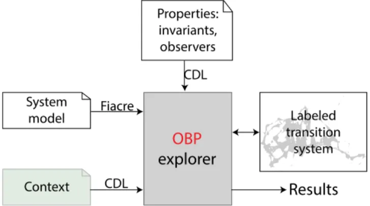
Our team develops and maintains a model-checking tool kit. The SUS is described using the Fiacre language [9], which enables the specification of interacting behaviours and timing constraints through timed-automata. Our approach, that we called Context-aware Verification, focuses on the explicit mod-elling of the environment as one or more contexts. Interaction contexts are described with the Context Description Language (CDL). CDL enables also the specification of requirements through predicates and properties. The requirements are veri-fied within the contexts that correspond to the environmental conditions in which they should be satisfied. All these devel-opments are implemented in the OBP tool kit [10] and are freely available1. Fig. 1 shows an overview of our approach.

CDL

OBP

explorer

_Results

Fig. 1. OBP Observation Engine overview

C. The Cruise-Control System

We will use the description and some of the requirements of an automotive Cruise-Control System (CCS) as a case study for this paper. Details can be found in [11].

1) SUS Model:

a) Functional Overview: The CCS main function is to adjust the speed of a vehicle. After powering the system on, the driver first has to capture a target speed, then it is possible to engage the system. This target speed can be increased or decreased by 5km/h with the tap of a button.

There are several important safety features. The system shall disengage as soon as the driver hits the brake/clutch pedal or if the current vehicle speed (s) is off bounds (40 < s < 180km/h). In such case, it shall not engage again until the driver hits a resume button. If the driver presses the accelerator, the system shall pause itself until the pedal gets released.

1_{OBP Languages and Tool kit website: http://www.obpcdl.org}

b) Physical architecture: The CCS is composed of four parts. A control panel component yields the controls needed to operate the system. An actuation component is able to capture the current speed and, once enabled, to adjust the vehicle speed towards the defined target. A health monitoring component detects critical events and relays them to the other components. A system center component acts as a controller. The car as a whole is a fifth component.

The control panel provides the driver with buttons needed to operate the system: PowerOn, PowerOff, SetSpeed, Resume, Disengage, IncrementSpeed, DecrementSpeed. The control panel should relay those operations to the system center. The actuation provides the tools for the system to interact with the vehicle. It can capture the current speed of the vehicle and set it as a target speed. One the CCS enabled, the actuation is responsible for controlling the vehicle speed accordingly. The health monitoring is responsible for monitoring the system and vehicle events that could impact the CCS behaviour: brake, clutch or accelerator pedals pressed or released, speed out of bounds. This component should relay such events to the system center which shall handle them.

The system center is the core of the CCS. It is responsible for handling events detected by both the control panel and the health monitoring components. To do so, it shall be able to impact the behaviours of all other components.

2) Requirements: Let us present two requirements of the CCS and their implementation using CDL: an observer au-tomaton for REQ1 (Fig. 2) and predicates for REQ2 (List. 1).

REQ1: When an event inducing a disengagement is

de-tected, the actuation component should not be allowed to control the vehicle speed until the system is explicitly resumed.

Fig. 2. Observer automaton for Req1.

REQ2: The target speed should never be lower than

40km/h nor higher than 180km/h. Listing 1. Specifying predicates for Req2.

1 2 p r e d i c a t e t a r g e t S p e e d I s U n S e t i s { 3 A c t u a t i o n @ U n S e t or A c t u a t i o n @ U n s e t S e t t i n g } 4 p r e d i c a t e s p e e d B e t w e e n 4 0 A n d 1 8 0 i s { 5 ( A c t u a t i o n : s e t P o i n t S p e e d >= 40 6 and A c t u a t i o n : s e t P o i n t S p e e d <= 1 8 0 ) 7 or t a r g e t S p e e d I s U n S e t }

III. QUERIES OVER ALABELLEDTRANSITIONSYSTEM A. Queries by example

1) A counterexample: Recall that an exploration explores the LTS in a brute-force manner in order to detect execution paths that violate specification properties. In a model-checking verification, the environment modelling should balance be-tween two important constraints: (i) the context has to cover

enough behaviours to be considered valid for a given property; (ii) it has to be small enough to allow an exhaustive exploration of the SUS composed with its environment. Hence we model an environment that combines a basic scenario and a pertur-bation scenario. The basic scenario is the main use case of the CCS that covers the functionalities needed to verify properties. The perturbation scenario is an alternative including changes of the vehicle speed within the allowed range or not, pressures on the pedals and the panel buttons. The perturbation scenario stresses the SUS with unexpected environment behaviours. Increasing and decreasing the vehicle speed is a continuous function that is typically provoking a state space explosion due to the infinity of possible values. Hence we have to transform the continuous variable in a discrete variable, for instance increasing or decreasing the speed by step of 5. Obviously, reducing or increasing this discretisation step will yield smaller or bigger LTS and we use this discretisation parameter as a way to make the exploration bigger to stress our tools.

A LTS is a set of nodes and edges. An edge is a transition between nodes. A node gathers information about a system state such as the variables values, the processes states, the messages in the queues. We call a configuration the data structure that holds this information. When the speed incre-ment or decreincre-ment is set to 5 km/h, the verification of the SUS design according to the two requirements presented in section II-C2 leads OBP to explore a LTS composed of 445 232 states and 672 247 transitions. Obviously, requirement REQ1 is violated in a bunch of configurations and OBP

yields any path that starts from the initial state and ends in a faulty configuration. Let us select the first faulty path, it ends at configuration 3128 and is composed of 211 transitions. There is no interest to see all the configurations details and because we are focussing on requirement REQ1, we might

want to see the path configurations where the observer state is changing. Only three configurations are involved and we have two successive paths: a path from configuration 0 to 2300 and a single-transition path from configuration 2300 to 3128 . We call a trail a succession of paths (2 in this case) between two configurations. Because the intermediate paths do not need to be expanded, all we need is a measurement of their size. The trail example is represented in Fig. 3.

Fig. 3. Visualization of a counterexample trail for requirement 1

2) Counterexample visualization: In a previous work [12], we wrote a specification of a visualization tool for traces. A prototype implementation has been made by a start-up company (OpenFlexo), that yields an open-source tool for models handling and information sources federation (see

http://www.openflexo.org). A central feature of trace visual-ization is the ability to represent traces according to different facets. A facet is an element, either belonging to the SUS design or a property or a predicate or an interprocess commu-nication (such as queue or an event). Facets can be queried and facet queries combined with logical operators. A facet query is usually a predicate related to the element type: variable values can be arithmetically checked, achieving a process state or an automaton state can be tested, event can be detected and so on. Very often, elements of interest are related to the fact that an element has its value changed and a special predicate changed highlights configurations where the element value has changed.

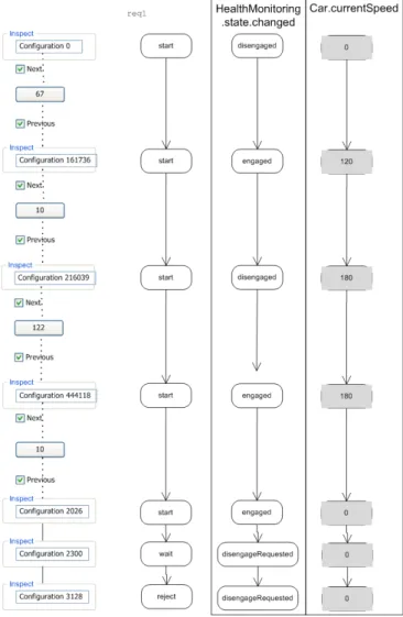
Fig. 4. Visualization of a counterexample for requirement 1

Fig. 4 shows a visualization of the counterexample trace presented in the previous subsection using two facets: an observer automaton and a process state. Because we want to understand the counterexample related to REQ1, we monitor

the HealthMonitoring process state (that induces a disen-gagement). We are also interested by the car speed and we display the current value of the variable currentSpeed for each configuration of the trail. Because it is often interesting to see what happened before a change, the user has explicitly unfolded the configuration 2026 that is a predecessor of the configuration 2300 (one of those where the HealthMonitoring process state has changed).

B. KriQL meta-model

1) Introduction: Our language is intended to ease traces understanding. A trace is a path in a LTS and because a LTS is essentially a Kripke structure [8], we call the language KriQL (Kripke Query Language). The design of KriQL was inspired from several sources. When we look at the LTS as a set of states, each state being represented by a configuration, we need a set-oriented language and SQL was a source of inspiration. A configuration or a configuration set can be projected along one or several configuration elements; a set can be restricted according to one or several predicates; union, intersection and difference of sets are required. When we look at the LTS as set of transitions, i.e. a graph, operations related to graphs are useful. Path existence, shortest or longest path between two nodes, path size are required. Because KriQL is intended to ease diagnosis, some operations stem from visualization needs. Paths can be folded and unfolded, step by step or entirely. Different visualizations issued from different facets have to be merged. Diagnosis practices such as looking at changing value or calculating the range of a variable yield also operations.

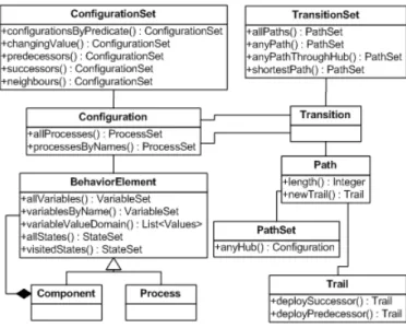
2) Operands and operators: We gathered these different sources in the KriQL core and its meta model is presented in Fig. 5. The meta-model corresponds to the design of an Application Programming Interface intended to provide the programmer with the minimal kit for implementing queries. Sets such as TransitionSet or ConfigurationSet are issued from the domain but some sets such as ProcessSet or VariableSet stem from technical requirements, essen-tially for handling query results.

Fig. 5. KriQL meta-model

C. Implementing the CCS

Each SUS is represented by a design that is refined iteratively. Thanks to the feedback of the model-checker and through the observation of traces, the designer is updating her design as a programmer tunes her program. The LTS structure is related with the design structure and the design structure allows the user to understand traces because it provides the user with structural information about the design: process names, variables names, constants and so on. Moreover traces

will be stored in a kind of database and the design structure yields the database structure. We discuss in this subsection the possible implementations of the design structure.

1) Relational DBMS: A relational DBMS stores data as table rows conforming to an application schema. Binding the design structure to an application schema can be accomplished in a generic or a specialized way.

A generic binding is applied to any design structure in the same manner; one set of tables is suitable for hosting data independently of the design structure. Reference to any par-ticular design construct such a process or a variable name, are provided via parameters as input of any operation. A generic binding specifies the set of operations to be made available to an application programmer explicitly.

A specialized binding produces a different set of tables upon a specific design structure. Hence the set of operations is dedicated to the design structure instead of being passed via parameters. A specialized binding does not specify the set of operations to be made available to an application programmer as this is dependent upon the design structure.

a) Generic binding: The database schema is not re-lated to a particular design structure but stems from the Fiacre language structure. A Configuration is made of several ProcessDataContainer, each of them related to a Process. A ProcessDataContainer holds one or several VariableValue either a scalar type (Boolean, Integer, . . . ) or an Array of VariableValue. Fig. 6 presents the class diagram of the generic binding that applies whatever the design structure is.

Fig. 6. Generic binding class diagram

Fig. 7. Excerpt of a specialized binding class diagram issued from the CCS b) Specialized binding: The database schema stems directly from the design structure. A Configuration is made of several XXX_Process, each of them related to a Fiacre process. A XXX_Process holds one or several attributes in a traditional way. Fig. 7 presents three processes of the specialized binding issued from the CCS structure.

2) Graph-based database: A graph database stores data as vertices and edges. Because we used the Neo4j system (http://Neo4j.com), we will use the Neo4j vocabulary, nodes for vertices and relationships for edges. A graph database does not have a schema as a relational database has. Neo4j language for querying graph database is called Cypher. Cypher queries find data that matches a specific pattern. A Cypher query anchors one or more parts of a pattern to specific locations in a graph using predicates and then flexes the unanchored parts around to find local matches [13]. Cypher queries are small graphs made from real nodes and relationships. Hence domain modelling in a graph database is isomorphic to graph modelling. According to [13], ”in a graph database what you sketch on the whiteboard is typically what you store in the database.”

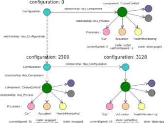
Fig. 8. A graph of three configurations

Because there is no schema, we have a kind of generic graph, but also specialized to each design structure be-cause a process node is labelled with the process name. A Configuration is made of a Component, each of them related to several XXX_Process. Fig. 8 presents the counterexample trail from Fig. 3. Three configurations are depicted; each is a small sub-graph: its root is a (blue) node labelled Configuration, the node has a re-lationship Has_component with a (rose) node labelled Componentthat holds relationships Has_processes with different XXX_Process nodes. As mentioned above, the graph sketched in the Fig. 8 is exactly the database structure. The configuration sub-graphs have the same structure and it might induce the reader to think that they share a common structure. It is true because the underlying LTS has the same structure for each node and each configuration sub-graph was created using the same pattern. However in another graph database application, it could have no common pattern and each sub-graph different from the others.

IV. IMPLEMENTATION ISSUES

In this section, we discuss about possible KriQL imple-mentations and we present related benchmarks.

A. Benchmark cases

We are using a discretisation parameter - the speed incre-ment - to produce LTS with different sizes: Small - 130,330 nodes and 197,045 transitions; Medium - 445,232 nodes and 672,247 transitions; Large - 1,103,952 nodes and 1,666,391 transitions. We made measurements on a PC running Ubuntu.

B. Loading Data

OBP stores the raw data issued from the model-checking exploration in two files (configurations and transitions) that need to be loaded in the database system before querying the LTS. Although storing the LTS in a database can be performed on-the-fly during the exploration, it is interesting to be aware of the overhead time required for the database store.

Configurations (nodes) can be stored with 3 architectures: generic relational, specific relational and graph; results are presented in Table I. In a relational model, storing transitions uses essentially a table with two columns, the configuration source and the configuration destination, hence it does not dif-fer between generic and specific bindings. Thus configurations can be stored with 2 architectures: relational or graph; results are presented in Table II. We can see that a graph loading is much faster than the loading of both relational bindings.

TABLE I. LOADING CONFIGURATIONS PERFORMANCES(seconds)

Generic Specific Graph Sma Mid Lar Sma Mid Lar Sma Mid Lar

326 1201 3373 152 655 1484 14 36 98

TABLE II. LOADING TRANSITIONS PERFORMANCES(seconds)

Relational Graph Small Mid Large Small Mid Large

17 56 141 1.38 2.38 3.94

C. Node queries

We selected 3 representative queries of nodes operations:

• configurationByPredicate - a restriction opera-tion that applies a predicate to a Configuraopera-tionSet source and returns nodes where the predicate is true. • changingValue - a side-effect restriction

opera-tion that monitors a configuraopera-tion element over a ConfigurationSet source and returns nodes where the monitored element (such as a variable or a process state) has its value changed regarding its predecessor. • variableValueDomain - a set construction operation

that gathers all values reached by a variable or a list of variables; it returns the set of values.

Relational queries use joins to combine data and dedicated structures such as indexes to improve join performances. With the generic binding, all data related to processes are hold in a single table, whether in a specific binding, each process has its own table that holds its data. Hence, we can expect that restriction queries over process elements will be faster with a specific binding because the tables size is reduced. Set construction operations such as variableValueDomain

require auto-join or recursive queries over the same table and will suffer of a same bias related to the tables size.

The concept of query in a graph database is a graph traversal. A traversal is the operation of visiting a set of nodes by moving between nodes connected with relation-ships. The traversal starts from selected nodes and col-lect the visited nodes along the relationship as results. The traversal continues its journey from one node to another via the relationships that connect them. The traversal stops when rules stop apply such as a depth size. Traversals are well-adapted for navigation along a path. When the whole graph needs to be traversed because the operator needs to process all nodes from a certain type (a restric-tion operator such as configurarestric-tionByPredicate or variableValueDomain), we can expect poorer perfor-mances of a graph database versus a relational one.

Node queries can be implemented with 3 architectures: generic relational, specific relational and graph; results are presented in Table III. Specific relational binding achieves very good performances; the changing operation time explodes for graph database implementation.

TABLE III. NODE QUERIES PERFORMANCE(seconds)

Gene. Spec. Graph Sma Mid Lar Sma Mid Lar Sma Mid Lar pred. 0.33 0.49 2.59 0.07 0.37 0.73 0.36 1.06 3.06 chng. 0.26 0.88 3.11 0.02 0.08 0.15 ˜7 exp. exp. dom. 0.91 1.26 ˜16 0.05 0.14 0.40 0.55 2 5.16

D. Edge queries

We selected 3 representative queries of edges operations:

• newTrail - a partitioning operation that splits a Path in a Trail (a sequence of Paths) according to a ConfigurationSet being the Trail milestones. • anyPath - a graph traversal operation that search a path

between two nodes over a TransitionSet; it returns the first Path that reaches the destination node. • allPaths - an exhaustive graph traversal

opera-tion that search all paths between two nodes over a TransitionSet; it returns a PathSet.

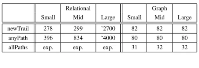
Edge queries are path walks and will require a massive use of joins in a relational implementation because edges are essentially couple of node identifiers (the source and the destination of the edge) stored in a single Transition table. There are no difference between a generic or a specific binding because the implementation is the same, but we can expect that the longer the path walk is, the poorer the performance will be because each step along the walk requires a join. The strength of a graph database is its ability to move between nodes con-nected with relationships without performance loss whatever the graph size. Thus we can expect excellent performances of a graph database versus a relational one.

Transitions can be stored with 2 architectures: relational or graph; results are presented in Table IV. Graph database implementation achieves very good performances, independent of the graph size; the allPaths operation time explodes for the relational implementation.

TABLE IV. EDGE QUERIES PERFORMANCE(milliseconds)

Relational Graph Small Mid Large Small Mid Large newTrail 278 299 ˜2700 82 82 82

anyPath 396 834 ˜4000 80 80 80 allPaths exp. exp. exp. 31 32 32

V. CONCLUSION

We performed benchmark measurements about node and edge queries with 3 typical queries in each case. We tested 3 different implementations, a generic binding and a specific binding to relational database (Postgres) and a graph database (Neo4j). Unfortunately, no implementations was successful for all test cases and we conclude for the necessity of a blended implementation: a relational specific implementation for node queries and a graph-based implementation for edge queries. Obviously, the main drawback of a redundant and blended implementation is the lack of synchronisation between both implementations. Because our goal is to query LTS in a front-end tool after the model-checker has provided its exploration results to the diagnostician, we do not need synchronisation and do not suffer of this drawback. Our current work aims to define the denotational semantics of KriQL.

REFERENCES

[1] C. Yuan, N. Lao, J.-R. Wen, J. Li, Z. Zhang, Y.-M. Wang, and W.-Y. Ma, “Automated known problem diagnosis with event traces,” in Proceedings of the 1st ACM SIGOPS/EuroSys European Conf. on Computer Systems. NY, USA: ACM, 2006, pp. 375–388.

[2] I. Herman, G. Melancon, and M. Marshall, “Graph visualization and navigation in information visualization: A survey,” IEEE Trans. on Visualization and Computer Graphics, vol. 6, no. 1, pp. 24–43, 2000. [3] A. K. Jain, M. N. Murty, and P. J. Flynn, “Data clustering: A review,”

ACM Comput. Surv., vol. 31, no. 3, pp. 264–323, Sep. 1999. [4] M. Hall, E. Frank, G. Holmes, B. Pfahringer, P. Reutemann, and I. H.

Witten, “The weka data mining software: An update,” SIGKDD Explor. Newsl., vol. 11, no. 1, pp. 10–18, Nov. 2009.

[5] F. Gilbert and D. Auber, “From databases to graph visualization,” in Information Visualisation (IV), 2010 14th International Conference, 2010, pp. 128–133.

[6] F. Holzschuher and R. Peinl, “Performance of graph query lan-guages: Comparison of cypher, gremlin and native access in neo4j,” in EDBT/ICDT 2013 Workshops. NY, USA: ACM, 2013, pp. 195–204. [7] D. Dominguez-Sal, P. Urbon-Bayes, A. Gimenez-Vano, S.

Gomez-Villamor, N. Martinez-Bazan, and J. Larriba-Pey, “Survey of graph database performance on the hpc scalable graph analysis benchmark,” in Web-Age Information Management. Springer, 2010, pp. 37–48. [8] M. Y. Vardi, “Automata-theoretic model checking revisited,” in

Pro-ceedings of the 8th Int. Conf. on Verification, Model Checking, and Abstract Interpretation. Springer-Verlag, 2007, pp. 137–150. [9] B. Berthomieu, J.-P. Bodeveix, P. Farail, M. Filali, H. Garavel, P.

Gau-fillet, F. Lang, and F. Vernadat, “Fiacre: an intermediate language for model verification in the topcased environment,” in ERTS 2008, 2008. [10] P. Dhaussy, F. Boniol, J.-C. Roger, and L. Leroux, “Improving model checking with context modelling,” Adv. in Software Engineering, 2012. [11] C. Teodorov, L. Leroux, and P. Dhaussy, “Context-aware verification of a cruise-control system,” in Model and Data Engineering. Springer International Publishing, 2014, pp. 53–64.

[12] V. Ribaud, “Specifications for trace visualization,” OpenFlexo, Tech. Rep., 2014.

[13] I. Robinson, J. Webber, and E. Eifrem, Graph Databases. O’Reilly Media, Inc., 2013.

[14] K. Es-Salhi, R. Boudaoud, C. Teodorov, and V. Ribaud, “KriQL a query language for labelled transition systems,” in submitted to AVOCS, 2015.