To link to this article : DOI:
10.1109/ICELMACH.2014.6960563
URL :
https://doi.org/10.1109/ICELMACH.2014.6960563
This is an author-deposited version published in:
http://oatao.univ-toulouse.fr/
Eprints ID: 11320
O
pen
A
rchive
T
oulouse
A
rchive
O
uverte (
OATAO
)
OATAO is an open access repository that collects the work of Toulouse
researchers and makes it freely available over the web where possible.
To cite this version: Allias, Jean-François and Llibre, Jean-François and
Henaux, Carole and Briere, Yves and Alazard, Daniel A global approach
for the study of forces developed by a tubular linear moving magnet.
(2014) In: ICEM 2014 - International Conference on Electrical Machines,
2 September 2014 - 5 September 2014 (Berlin, Germany)
Any correspondence concerning this service should be sent to the repository administrator:
Abstract -- A global approach for the study of forces
developed by a tubular linear moving magnet actuator for a low speed and high force application is described. We used here an easy analytical approach made with the Ampere’s law to give the field distribution done by permanent magnets in the airgap. In order to calculate the effort developed by the moving part we used the Laplace force which takes into account the field distribution calculated previously and the current distribution on the stator. The results are validated extensively by comparison with finite element analysis. The analytical field solutions allow the prediction of the thrust force. This facilitates the characterization of tubular machine topologies and provides a basis for comparative studies, design optimization, and machine dynamic modeling.
Index Terms-- Laplace Equations, Linear actuator,
Optimization, Permanent Magnet Motor I. INTRODUCTION
LECTRICAL systems are more and more reliable and they are worthy of interest for some applications which try to reduce the embedded weight. If we compare with mechanical or hydraulic systems, maintenance and integration are easier thanks to the compactness of the electrical actuators. These advantages push for the development and the multiplication of electrical technologies in embedded systems. This paper deals with the presentation of a linear actuator for an embedded application. The actuator requirements have to provide a high force per unit of mass in a low speed range for a power consumption of 100 (W).
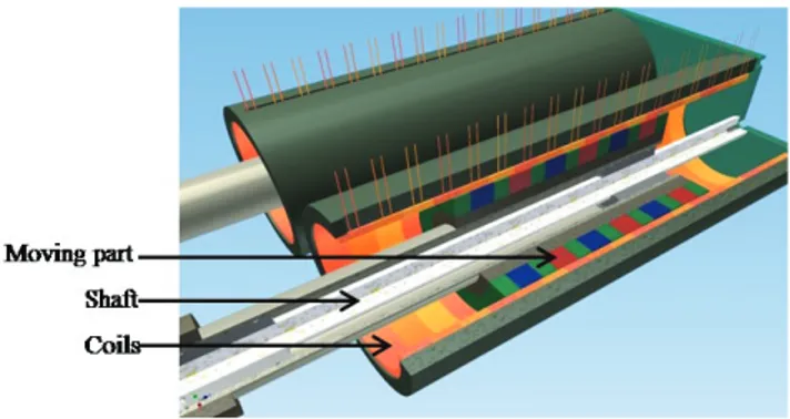
The proposed structure for this application is a tubular linear moving magnet actuator (MMA) which presents all the characteristics of a synchronous permanent magnet machine as in [1]-[2]-[3]. The Fig. 1 shows the chosen structure. The moving part is composed of permanent magnet radially magnetized fixed to a tubular magnetic circuit. The stator is composed of ring shaped coils which are assembled on a smooth magnetic circuit without teeth and slots. Two MMA mounted in parallel are shown in Fig. 1.
Among various linear machine configurations, tubular machines with permanent magnet excitation have a number of distinctive features such as a high force density and excellent control characteristics, which make them an attractive candidate for applications in which dynamic performance and reliability are crucial like in [4]. On the scientific literature as in [1]-[5]-[6]-[7], the analytical
This work was supported in part by the A.N.R. (Agence Nationale de la Recherche).
J. F. Allias, J. F. Llibre, and C. Henaux are with Université de Toulouse ; INPT, UPS ; CNRS LAPLACE (Laboratoire Plasma et Conversion d’Energie) ; ENSEEIHT, 2 rue Charles Camichel, BP 7122, F-31071 Toulouse cedex 7, France.
Y. Briere, and D. Alazard are with Institut Supérieur de l’Aéronautique et de l’Espace, Département DMIA, 31055 Toulouse, France.
models are based on the Poisson’s equation where the magnetic field distribution created by permanent magnets is developed in Fourier series. This kind of equations leads to solutions using the Bessel functions. In the aim of finding the linear force developed, we have to apply the Maxwell stress tensor which gives very precise results in spite of the hardness and the computation time of this model. In [8]-[9]-[10], the magnetic computation is performed using a reluctance magnet network. We found it interesting to use a simplest model based on Gauss’s law and Laplace’s force that consumes little computation time.
In the first section of this paper we will present this model based on the chosen structure of the machine which respect the set of specifications. In the second section, an optimization process is undertaken to determine the dimensional characteristics of the structure. In the third section, we will compare the theoretical results with the simulation results obtained by finite elements done with the Ansys software. Finally, the last section presents the conclusion and perspectives of the work.
Fig. 1. Tubular moving magnet actuator.
II. PREDIMENSIONING:ANALYTICAL CALCULATION
A. Set of specifications
For this application we have to comply with a set of constraints such as dimensions, duplications, forces, stroke, speed, temperatures and force ripples constraints. The application requires that the system is redundant. Thus two actuators are implemented in parallel, each of them has to develop 55 (N) without ripples for an electric power consumption of 100 (W). These two actuators are embedded in a box of which dimensions are 165*304*304 (mm). So, the volume and the mass of the armature have to be minimized. The stroke of the moving part must be of ∓ 90 (mm) and the maximum speed has to reach 0.5 (m. s"#). As we said before, there are also
temperature constraints for coils and magnets. Of course, it is important to not exceed the Curie temperature of the magnets which could be the cause of a premature demagnetization and could be highly harmful for the well-functioning of the actuators. A precise study is necessary to dimension the variety of magnets we are going to use like
A global approach for the study of forces
developed by a tubular linear moving magnet
actuator
J. F. Allias, J. F. Llibre, C. Henaux, Y. Briere, D. Alazard
Samarium-Cobalt or Neodymium-Iron-Boron. In the same time, the winding temperature does not have to reach 180 (°C).
B. Electromechanical characteristics and shape of the actuator
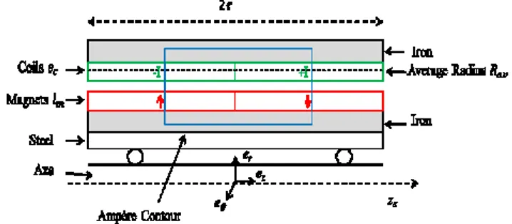
According to these requirements, the chosen structure is a tubular linear moving magnet actuator. Because the magnets are radially magnetized and the coils are ring shaped without saliency, we can use the Ampere theorem around a contour applied to a half section of the axisymmetric actuator in the (O, ••, • ) plane and calculate the flux density in the airgap. Then, we are able to calculate the Laplace force on the elementary pattern presented in Fig. 2, whose dimensional characteristics are given in Table I. In order to simplify, we consider only one pole pair of magnets and two coils supplied by opposite continuous currents. The effort determined on the elementary pattern can be generalized over all the structure if we multiply by the number of pairs of poles !. In order to have a constant effort, each coil surface will be divided in three and will receive sinusoidal currents with 120° phase shift, see Fig. 4. We will see later in this paper how we get this effort and his value.
Fig. 2. Elementary pattern and Ampere contour.
TABLE I
DIMENSIONAL CHARACTERISTICS OF THE MACHINE
Name Definition
"# Magnet thickness
$% Moving part external radius
& Airgap thickness &' Coil thickness
"(= & + &' Airgap and coil thickness
$) Stator external radius
*,- Average radius (half of the coil)
. One pole length
The pre-design of the actuator consists in the choice of a simple theoretical model based on the Ampere’s law. The linear force produced is given by the Laplace force defines by the following expression:
/0
1= 2. /4 × 5
(1)where 5 is the pseudo-vector of magnetic field, I the total current in the coil, /4 an infinitesimal part of the current trajectory and /01 the infinitesimal Laplace force. To reach the total force applied over the contour we need to integrate around the windings (the angle θ is varying from 0 to 2π).
We also integrate at the middle of the coils at the average radius *,-. Thus, we consider a current sheet equivalent to the coil current density. It means that the Laplace force is:
0
1= 6 2. *
,-. 78. •
9× 5
:;<
(2)
The waveform created by the radial magnetization pattern and the displacement of the moving part is considered as strictly sinusoidal as in [11]-[12]-[13]. We can traduce this mathematically by:
>?(A%) = CD#. sin Eπτ (A%)H . ••
(3)
It is easy to write the following relation between axes: A% = AI− A%I (4)
where A) is the fixed axis tied to the stator, A% is the moving axis tied to the moving part and A%I shows the position of the moving part (Fig. 3) in relation to the stator expressed by:
A%I= L. M (5)
where L is the linear speed and M the time. CD# is the peak value of the residual flux density of the magnet. Finally, we can write:
C#(A%) = C#(AI, A%I) = CD#. OPQ ER. (AI− A%I)H (6)
Fig. 3. Representation of axes.
The coils are molded and are tied to the stator at the ends. They have got ring shape around the AI axis. The stator has no teeth in order to reduce the saliency effect. In the following of this paper we will employ the term slot area which represents the area cross section of the coil supplied by current namely:
S)TUV= &'. . (7)
Copper wire is crossed over a current 2 and we make a difference between the two currents densities C'UWT and C)TUV which respectively represent the current densities in a coil and in a slot expressed in (A. mmY:). The magneto-motive force Q2 with Q the number of turns per slot is equal to:
Z[. C'UWT. S)TUV= Q2 (8) where Z[ is the slot fill factor equal to the ratio II\]^_
`_]a.
C. Magnetic flux densities
The following assumptions are made. For a magnetic point of view, copper is similar as air. In order to simplify
the calculation, we assume that the iron permittivity is infinite. Then, as the iron flux density has got a finite value, the magnetic excitation in the iron is equal to zero.
Finally, the magnetic flux densities in the air region Be
and in the magnet region Bm are defined as in [14] by:
and,
Our application needs to develop high forces then we are going to use rare earth magnets like Neodymium-Iron-Boron, with •
̂
•= 1,4 (•) or Samarium-Cobalt, with •̂
•= 1,1 (•). Here, µ!= 4π. 10#$ (%. •#&) and µ'depends on the magnets and is often between 1,03 and 1,15. From (10), we consider that we are on the linear part of the hysteresis curve.
Then in this linear problem we use the superposition theorem. We will not consider the coils and we can write the Ampere’s law:
%*. +*+ %/. +/= 0 (11)
The Gauss’s law gives:
2*. 6*= 2/. 6/ (12)
where 6* and 6/ are respectively the flux exchange areas in the airgap and in the magnets.
Finally, the magnetic field in the airgap is directly proportional to the residual flux density by a coefficient named 7* which only depends on the dimensions such as:
7*(8) = 1 96*(8) 6/ + µ'. + *(8) +/ :
(13) and, ;<(8, >?, >@?) = 7*(8). AB(>?, >@?)
(14)
D. Linear stress calculation
To determine the linear stress, the Laplace force is applied at the middle of the coils, at CDE radius (the real airgap F is small compared to the coil width FG). Finally, as the coil is attached to the stator, this effort is the one which is applied to the moving part. By using (2), (8), and (14), the Laplace force depends on >? and >•6 and is given by:
HI(>?, >@?) = 2π. KL(>M)
. C
NO. ;<(C
NO, >
P, >
•6)
(15) where, KL(>M) is given by (8) with:•GQRS(>M) = T+•UVW+, >−•UVW+, >?∈ [0, τ]
?∈ [τ, 2τ] (16)
Finally, to reach the total force of the linear actuator, with opposite continuous current, in relation of the position of the moving part >@? it is necessary to multiply by the
number of half pairs of poles 2\ and integrate over a half period of magnets i.e. a pattern of [0, τ]. Due to the symmetry with the supply of the coil by opposite continuous current, the total force of the moving part is:
H^_`(>@?) = 2\.1τ a bc(>?, >@?). d
! e>?. <f (17)
After integration we can get the following result:
H^_`(>@?) = 8. \. KL. CDE. 7*. •h/. cos jπτ . >@?k . <f (18)
Then, with the coils supplied by a three phase sinusoidal current, as we said in II.B. the total force reached by the moving part is equal to:
Hl_`(>@?) =3\τ . m aR.dn bc(>?, >@?)R (R#&).dn
p
Rq&
e>?. <f (19)
Taking into account the symmetries, this gives: Hl_`(>@?) =6\τ . m aR.dn bc(>?, >@?)R (R#&).dn n Rq& e>?. <f (20) where: HI(>6,>•6)R= 2π.KLW.CNO.;<
(C
NO,>
P,>
•6)
(21) This force depends on KLR which is explained in (22). The •GQRSt current densities vary with i from 1 to 6 in (19) orfrom 1 to 3 in (20). In (16), we have defined on the two coils which total length is 2 (corresponding to one pole pair, see Fig. 2), two opposite current densities depending on the >? axis. With a three phase supply, each slot is divided in three (see Fig. 4) and we define, for the total length 2 six different current densities as a function of the time and of the >? axis. These current densities •GQRSt, where W represents each of the six slots areas, are shown in Fig. 4.
Fig. 4. Three phase supply of the coils.
Each coil is supplied (like in [15] ) by: 2*= µ!. %* (9)
| !"| = #$.%&'()3 . *+,("'-* (22) and then, ⎩ ⎪⎪ ⎨ ⎪⎪ ⎧ +,("'4(6) = 3. !8 #$. %&'(). sin ( : ; . <>?+ φ8) +,("'B(6) = −3. !D #$. %&'(). sin ( : ; . <>?+ φD) +,("'E(6) = 3. !F #$. %&'(). sin ( : ; . <>?+ φF) (23)
After calculation, and considering currents with 120° phase shift, we observe that the force with a three phase supply is constant and does not depend on <G%:
HDIJ= 6. L. #$. +,("'. %&'(). MNO. PQ. +RS (24)
Thus:
HDIJ=34 H8IJ (25)
In order to simplify and to save computation time, the simulations and the optimizations will be performed for a single phase and opposites continuous currents configuration. The specifications required for the linear actuator is to achieve HDIJ=55 (N) with a three phase sinusoidal supply which eliminates force ripples. So, for a single phase configuration the dimensioning force to reach is:
H8IJ =UD. 55 = 73 (N).
III. OPTIMIZATION OF THE STRUCTURE
With the aim of getting the best compromise, we need to optimize the structure of the linear actuator by the method of multi-objective optimization. We realized all the optimization for samarium cobalt magnets (+
̂
Z= 1,1 (G)). Our objectives are to maximize the force and to minimize the mass and the thermal parameter that we will define later. The constraints of our problem are dimensional constraints like the size of the box, magnetic constraints (the value of the magnetic flux density in the iron should not exceed the material saturation). In mathematical terms our optimization problem can be traduced as in [16] by the following expressions: ] min ^∈ℝab(c) d"(c) ≤ 0 ∀h ∈ {1, … , j} ℎl(c) = 0 ∀o ∈ {1, … , J} (26)where b is the objective function we have to minimize, d and ℎ are respectively the functions which represent the inequality constraints and the equality constraints. The variable fixed is c, j and J represent respectively the number of inequalities and equalities equations. Here c ∈ ℝp and represents all the variables of our optimization
problem, that is to say for example ( +,("', L, ;, qS… ).
In our problem, one of the three objectives is the mass of the linear actuator:
r(c) = t ρv. π. (x"F− x"y8F ). z" ~
"•8
(27)
where z" and €" are respectively the length and the densities of each layer (iron yokes, magnets, coils…). The number of layers is n and each layer is bounded by the radius ri-1 and ri
(with r0 = 0).
One objective is the thermal parameter mentioned above. This parameter is called Gℎ, such as:
Gℎ(c) = •(c). +,("' (28)
where •(c) is the current density per unit of length, see [17].
We can write the b function like in [16]: b(c) = −max„HH8IJ(c)
8IJ†+
r(c)
min(r) +min(Gℎ)Gℎ(c) (29) There is a set of constraints ( j+ J) like: flux density saturation constraints and dimensional constraints. But the three main constraints are force, mass and current density:
‡+,("'H8IJ≤ 10 (A. mm≥ 73 (N)yF)
r ≤ 3.75 (kg) (30)
To realize this optimization we need to make as many calculations as we have objectives. The goal is to find an extremum for each following objective: "max„H8IJ†", "min(r) " and "min(Gℎ)". Finally, we make one more multi-objective calculation. In order to realize this optimization, we used the optimization toolbox of the Matlab software. We also used the bZh •Ž function with the dqŽ••q ‘’•x•ℎ module. We will present our results in the next section.
IV. SIMULATION AND RESULTS
We made the simulations with the Ansys software [18] in quasi-static. It is here a 2D axisymmetric simulation with a triangular meshing. In these simulations a single phase continuous current is set in order to calculate the maximum force reached by the linear actuator. It is also a way to check if the hypothesis of the sinusoidal waveform created by radial magnetization pattern is correct (3).
In order to validate the theoretical model, we have simulated the MMA for further configurations like in [19]-[20]. For each MMA geometry, we tried to choose different configurations by varying the length, the number of poles and the size of each layers. Table II shows the results and relatives errors of three different geometries. The first geometry, called GEOM1, has a short moving part with one pair of pole. In the second geometry, called GEOM2, we conserved the characteristics of the first geometry, the moving part is longer than in the first one. In the third geometry, called GEOM3, we changed the sizes of the moving part and of the external radius x&. There are also two pairs of pole. Fsimu is the force calculated thanks to
Ansys software [18] and Fth is the peak value of the force
calculated using (18) with the help of Matlab software. For these three configurations, the relative error between these efforts is less than 2%. Thereby, we are more confident on the analytical model. We can use it for the optimization process in order to find an optimized structure.
TABLE II
COMPARISON BETWEEN SIMULATIONS AND THEORETICAL MODEL FOR DIFFERENT GEOMETRIES
• !"# (N) •$% (N) &%
GEOM1 32.6 33.04 -1.33
GEOM2 55.99 55 1.8
GEOM3 73.10 72.04 1.47 Table III compares the results of each optimization, that is to say that the second, third and fourth columns represent each mono-objective optimization and the fifth column gives the results of the multi-objective optimization. It should be noted that the fourth and fifth column are the same. It means that the thermal parameter is the most restrictive objective of the optimization.
TABLE III
TABLE OF THE RESULTS OF EACH OPTIMIZATION CALCULATION •()% * +ℎ Multi-objective -"(mm) 5.4 5 11.7 11.7 0$ (mm) 24.4 24 30.7 30.7 23 (mm) 2.58 2.2 2.13 2.13 0 (mm) 32.5 31.7 38.3 38.3 τ (mm) 38.3 15.3 23.3 23.3 435!6 (A. mm89) 10 10 8.37 8.37 : 1 2 1 1 •()% (N) 108 73 73 73 * (kg) 3.75 3.17 3.75 3.75 +ℎ (A9. m8;) 1.22(( 8.232(< 3.442(< 3.442(<
Now that we are sure that we have reached an extremum that meets all the constraints, we are able to make a finite element simulation of the optimal structure. To have an idea of the simulated structure in two dimensions, we show on Fig. 5 the 2D flux lines.
Fig. 5. 2D Flux lines of the simulated MMA structure.
We putted here the Dirichlet conditions on the edges. That means that the vector potential on θ direction (Fig. 2) is equal to zero.
Fig. 6 shows the result of flux density created by permanent magnets radially magnetized in the airgap, took on the half of the coils, with the Ansys software. This curve permits to verify the hypothesis given in (3).
Fig. 6. Flux density created by permanent magnets in function of the position relative to the Zs axis.
Theoretically, when the armature is radially magnetized, the repartition of the flux density in the airgap should be like square or trapezoidal waveform; but when the length of the magnet is short the hypothesis of the sinusoidal waveform created by the PM can be done as we can see on Fig. 6. In order to improve the sinusoidal shape of the waveform we can use the work done in [12] with keeping the pole pitch (2τ) constant. We can now test our analytical model based on the calculation of the force created with single phase and opposite continuous currents. Fig. 7 shows the results of the simulations forces and calculated force.
Fig. 7. Force in single phase opposites continuous current in function of the stroke.
The Ansys software [18] allows us to calculate force with two distinctive numerical methods such as “virtual work” and “Maxwell stress tensor”. If the results of these two methods are tied in, as in Fig. 7, it means that the mesh is quite good. Thus, we are able to compare the theoretical curve, with the two other ones which represent the numerical results. About the maximal force, our analytical model seems to give very precise results. We observe a small gap between theoretical force and numerical forces which means that the force felt in single phase, with opposite continuous current, is near from a cosinus function as the theoretical result deduced from (18). In order to validate (24), and including the fact that Ansys is a finite element calculation software which only permits to make quasi-static simulations, we decided to recreate a three
phases sinusoidal current supply with continuous currents as in Fig. 8.
Fig. 8. Creation of a three phases sinusoidal current supply with continuous currents.
On Fig. 8, we see in red the displacement of the moving part relative to the •• axis. We also see the repartition of
continuous currents in each slot to recreate three phases sinusoidal supply. Fig. 9 shows the results of the simulations done with the current repartition given in Fig. 8, when the moving part moves a distance 2 .
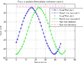
Fig. 9. Forces in three phase continuous current in function of the stroke
The plot 1 in blue and the plot 2 in green of Fig. 9 show the results of the Maxwell stress tensor and virtual work forces developed respectively with the first and second current distribution of Fig. 8. When the actuator will be supplied by a three phase sinusoidal current and field oriented control, the resultant force will be a constant effort (equal to the peak value of the sinusoidal function) represented by the pink curve on Fig. 9. One can observe a difference between the theoretical and simulated forces !"#$ which are equal respectively to 51.8 (N) and 55 (N).
Thus, the relative difference is equal to 5.8 %. It can be explain by the fact that the Ansys software takes into account the iron magnetic flux density that we did not consider on our analytical model. There is also the fact that we only consider the fundamental waveforms of the current and the flux density in the airgap.
!
3%ℎ−()*+= 51.82
(N
)and,
!
3%ℎ−/ℎ04= 55
(N
)Thus, the relative error on the three phase force is : 6%=−5.8 %
V. CONCLUSION
In this paper, we have presented an analytical approach of the calculation of force which can be applied to slotless synchronous permanent magnet machines where the waveform created by PM is close to a sinusoidal function. We used it for the dimensioning of a tubular linear moving magnet actuator devoted to an embedded application. A set of constraints have to be met like: total force expected, no force ripples, bulk, mass and thermal limitations. In a first step, we have made a modeling based on an Amperian model of the structure. This model offers the advantages to be faster to solve than Poisson equation and to consume less computation time in a multi-criteria optimization calculation. In a second step, the analytical results and especially the linear effort developed were verified by a 2D finite element analysis. Then, a multi-criteria optimization of the actuator structure based on an objective function assuming a set of constraints has been carried out. This optimization allowed us to give the dimensions of the actuator that almost meets the specifications (5.8% difference between the expected effort and the calculated effort). In our future work, we intend to improve the analytical modeling considering the harmonic orders greater than one for the fields. Moreover, based on this study, a prototype has to be built and experimental tests have to be performed.
VI. REFERENCES
[1] S. M. Jang, J. Y. Choi, S. H. Lee, H. W. Cho, and W. B. Jang, “Analysis and experimental verification of moving-magnet linear actuator with cylindrical Halbach array”, IEEE Trans. On
Magnetics, vol. 40, no. 4, pp. 2068-2070, Jul. 2004.
[2] H. Ben Ahmed, B. Multon, and M. Ruellan, “Actionneur linéaires directs et indirects”, “revue 3EI”, pp. 38-58, septembre 2005. [3] Y. Amara, G. Barakat, “Analytical modeling of magnetic field in
surface mounted permanent-magnet tubular linear machines”, IEEE
Trans. On Magnetics, vol. 46, no. 11, pp. 3870-3884, Nov. 2010.
[4] J. Wang, G. W. Jewell, “A general framework for the analysis and design of tubular linear permanent magnet machines”, IEEE Trans.
On Magnetics, vol. 35, no. 3, May 1999.
[5] N. Bianchi, “Analytical computation of magnetic fields and thrusts in a tubular PM linear servo motor”, IEEE Industry Application
Conference, Rome Italy, Vol. 1, pp. 21-28, 8-12 Oct. 2000.
[6] Y. Boutora, R. Ibtiouen, and N. Takorabet, “Analytical model of parallel magnetized magnet segments of surface PM slotless machine”, IEEE XXth International Conference on Electrical Machines (ICEM 2012), Marseille France, pp. 2772-2778, 2-5 Sept.
2012.
[7] D. L. Trumper, W. J. Kim, and M. E. Williams, “Design and analysis framework for linear permanent magnet machines”, IEEE
Trans. On Industry Applications, vol. 32, no. 2, March/Avril 1996.
[8] N. Bianchi, S. Bolognani, F. Tonel, “Design criteria of a tubular linear IPM motor”, IEEE Electric Machines and Drives Conference
(IEMDC 2001), Cambridge England, pp. 1-7, 17-20 June 2001.
[9] N. Bianchi, S. Bolognani, D. Dalla Corte, F. Tonel, “Tubular linear permanent magnet motors: an overall comparison”, IEEE Trans on
Industry Applications, vol. 39, no. 2, pp. 466-475, March/April 2003.
[10] H.W. Lee, C.B. Park, B.S. Lee, and H.J. Park, “Exit end effect reduction of a linear induction motor for the deep underground GTX”, XIX International Conference on Electrical Machine-ICEM
2010, Rome
[11] S. Dwari, L. Parsa, and K. J. Karimi, “Design and Analysis of Halbach array permanent magnet motor for high acceleration applications”, IEEE Electric Machines and Drives Conference
[12] Steven A. Evans, “Salient pole shoe shapes of interior permanent magnet synchronous machines”, XIX International Conference on
Electrical Machine-ICEM 2010, Rome
[13] Y. Okada, H. Dohmeki and S. Konushi, “Proposal of 3D-stator structure using soft magnetic composite for PM motor”, XIX
International Conference on Electrical Machine-ICEM 2010, Rome
[14] L. Jian, K. T. Chau, C. Yu, and W. Li, “Analytical calculation of magnetic field in surface-inset permanent magnet motors”, IEEE
Trans. On Magnetics, vol. 45, no. 10, October 2009.
[15] F. Kelemen, L. Strac and S. Berberovic, “Influence of a delta connected winding on magnetizing currents of a five limb core power transformer”, XIX International Conference on Electrical
Machine-ICEM 2010, Rome
[16] E. Fitan, F. Messine, and B. Nogarede, “The electromagnetic actuator design problem: a general and rational approach”, IEEE
Trans. On Magnetics, vol. 40, no. 3, May 2004.
[17] B. Nogarede, “Etude des moteurs sans encoches à aimants permanents de forte puissance à basse vitesse”, These de l’institut polytechnique de Toulouse, 1990.
[18] Ansys Multiphysics - APDL (Ansys Parametric Design Language) [19] S. Alshibani, R. Dutta, V. G. Agelidis, “An investigation of the use
of a Halbach array in MW level permanent magnet synchronous generators”, IEEE XXth International Conference on Electrical Machines (ICEM 2012), Marseille France, pp. 59-65, 2-5 Sept. 2012.
[20] J. Wang, C. Li, Y. Li, and L. Yan, “Optimization design of linear Halbach array”, IEEE International Conference on Electrical
Machines and Systems (ICEMS 2008), Wuhan China, pp; 170-174,
17-20 Oct. 2008.
VII. BIOGRAPHIES
Jean-François Allias was born in 1988 in Toulouse, France. He received
the Engineer’s degree in Electrical Engineering from ENSEEIHT (Ecole Nationale Supérieure d’Electronique, d’Electrotechnique, d’Informatique, d’Hydraulique et de Télécommunication) in Toulouse, France, in 2012. He is Ph. D. student in GREM3, research group of the Laplace laboratory, in Toulouse. His field of competence is centered around the design of magnetic structure by optimization process.
Jean-François Llibre received the Ph. D. degree in Electrical Engineering
from National Polytechnic Institute of Toulouse in 1997. He is a lecturer since 1998 and teaches electrical engineering in the University Institute of Technology of Blagnac near Toulouse since 2003. He joined the GREM3
electrodynamics research group of LAPLACE laboratory in 2010. His actual main research interests concern the modeling, the analytical field calculation, the optimal design in electrical machines field.
Carole Henaux received the Dipl. Ing. Degree in Electrical Engineering
from ENSEEIHT, Toulouse, France, in 1992 and the PHD degree from the National Polytechnic Institute of Toulouse in 1996. She is now a Lecturer with the Electrical Engineering department of INPT / ENSEEIHT. She teaches Electrical Machines modeling and is also the head of the Electrodynamics – GREM3 research group of INPT-ENSEEIHT-LAPLACE, Toulouse. The group is of 9 permanent academics working in the fields of electromechanical energy conversion, with particular interest in novel techniques and design methodologies such as electroactive materials, composite magnetic materials, electroactive fluids, analytical field calculation, optimal design.
Yves Briere was born in Toulouse (France). He was graduated from the
Ecole Nationale Supérieure d'Electrotechnique Electronique et Hydraulique de Toulouse (ENSEEIHT) in 1990. He received a Phd Degree in robotics from SUPAERO (École Nationale Supérieure de l'Aéronautique et de l'Espace) in 1994 with a research dedicated to teleoperation with force feedback hosted by ONERA (Office Nationale d'Etudes et de Recherche Aérospatiale) and granted by CNES (Centre Nationale d'études Spatiales). After a one year post doc in the Stanford Robotics Laboratory he was hired at a full time professor at the University of Pau for three years. He has been at ISAE (Institut Supérieur de l'Aéronautique et de l'Espace, Toulouse, France) since 2000. He teaches control and estimation and his main research interest is related to control of mobile robots.
Daniel Alazard was born in Tarbes (FRANCE). He was graduated from
the Ecole Nationale Supérieure des Arts et Métiers (golden medal) in 1986 and received the Master in Advanced Automatic Control and Systems from SUPAERO (Ecole Nationale Supérieure de l’Aéronautique et de l’Espace) in 1987. Since 1989, he is a research scientist at ONERA (French Aerospace Lab) - Department of System Control and Flight Dynamics (DCSD) in Toulouse. Between 1997 and 2000, he was at the head of the research group Control and Integration. Since 2000, he is full Professor at ISAE/SUPAERO. His main research interests concern robust control, flexible structure control and their applications to various aerospace systems. He passed the Accreditation to Supervise Research in 2003.