O
pen
A
rchive
T
OULOUSE
A
rchive
O
uverte (
OATAO
)
OATAO is an open access repository that collects the work of Toulouse researchers and
makes it freely available over the web where possible.
This is an author-deposited version published in :
http://oatao.univ-toulouse.fr/
Eprints ID : 12147
To link to this article : doi: 10.1007/s00162-014-0330-9
URL :
http://dx.doi.org/10.1007/s00162-014-0330-9
To cite this version : Andersson, Fredrik and Carlsson, Marcus and
Tourneret, Jean-Yves and Wendt, Herwig A New Frequency
Estimation Method for Equally and Unequally Spaced Data. (2014)
IEEE Transactions on Signal Processing, vol. 62 (n° 21). pp.
5761-5774. ISSN 1053-587X
Any correspondance concerning this service should be sent to the repository
administrator:
[email protected]
A New Frequency Estimation Method for Equally
and Unequally Spaced Data
Fredrik Andersson, Marcus Carlsson, Jean-Yves Tourneret, and Herwig Wendt,
Abstract—Spectral estimation is an important classical problem
that has received considerable attention in the signal processing literature. In this contribution, we propose a novel method for esti-mating the parameters of sums of complex exponentials embedded in additive noise from regularly or irregularly spaced samples. The method relies on Kronecker’s theorem for Hankel operators, which enables us to formulate the nonlinear least squares problem associated with the spectral estimation problem in terms of a rank constraint on an appropriate Hankel matrix. This matrix is generated by sequences approximating the underlying sum of complex exponentials. Unequally spaced sampling is accounted for through a proper choice of interpolation matrices. The resulting optimization problem is then cast in a form that is suitable for using the alternating direction method of multipliers (ADMM). The method can easily include either a nuclear norm or a finite rank constraint for limiting the number of complex exponentials. The usage of a finite rank constraint makes, in contrast to the nuclear norm constraint, the method heuristic in the sense that the problem is non-convex and convergence to a global minimum can not be guaranteed. However, we provide a large set of numerical experiments that indicate that usage of the finite rank constraint nevertheless makes the method converge to minima close to the global minimum for reasonably high signal to noise ratios, hence essentially yielding maximum-likelihood parameter estimates. Moreover, the method does not seem to be particularly sensitive to initialization and performs substantially better than standard subspace-based methods.
Index Terms—Alternating direction method of multipliers,
frequency estimation, Hankel matrix, irregular sampling, Kro-necker’s theorem, missing data, spectral estimation.
I. INTRODUCTION
S
PECTRAL estimation is a classical problem that appears in an immense variety of problems encountered in signal and image processing applications. These applications includeas-F. Andersson and M. Carlsson are with the Centre for Mathematical Sci-ences, Lund University, 22100 Lund, Sweden (e-mail: [email protected]; marcus. [email protected]).
J.-Y. Tourneret is with the Signal and Communication Group of the IRIT Lab-oratory, University of Toulouse, ENSEEIHT, 31071 Toulouse Cedex 7, France (e-mail: [email protected]).
H. Wendt is with the CNRS and with the Signal and Communication Group, IRIT Laboratory, CNRS UMR 5505, University of Toulouse, ENSEEIHT, BP 7122, 31071 Toulouse Cedex 7, France (e-mail: [email protected]).
Digital Object Identifier 10.1109/TSP.2014.2358961
tronomy, radar, communications, economics, medical imaging, spectroscopy, to name but a few, (e.g., see [1] and the references therein). One important class of spectral estimation problems arises for signals that can be modeled as sums of complex ex-ponentials (or sinusoids) in noise, i.e., for signals that admit the parametric model
(1) where is a complex frequency mode with fre-quency parameter and damping parameter , is a com-plex amplitude and is an additive noise term. Note that the model (1) includes the case of exponentially damped sig-nals defined by , with important applications notably in spectroscopy (see for instance [2], [3] and references therein). The main goal of frequency estimation is to estimate the values of the parameter vector from a vector of values defined by (1) sampled at positions , where is the number of samples. In the present contribu-tion, the approach to this problem in addition has the capacity to treat the case when is sampled at unequally spaced posi-tions , a frequently appearing situation in many areas, for instance in spectroscopic data analysis [2], [3] and synthetic aperture radar [4], [5]. See also [6] for more examples. Note that once estimates of have been obtained, the vector of complex amplitudes can be determined by simple linear regression, hence the focus lies on the estimation of the modes .
The estimation problem associated with (1) has been studied extensively for the case of regular sampling. Many estimation methods exist, e.g., see [7]–[12] and [1] for an overview. Some of these methods can be adapted to the unequally spaced sam-ples, cf., [13] for a review. One prominent class of estimation techniques for the model (1) is given by subspace methods, in-cluding the popular MUSIC [14], ESPRIT [15] and min-norm [16] methods. These methods are constructed on the basis of the sample covariance of and rely on the assumption that the noise is white. Subspace methods can provide high-resolution estimates (i.e., below Nyquist sampling frequency resolution and equal to numerical precision in the noise free case). How-ever, they are known to be statistically suboptimal [17]–[20] and cannot be applied to unequally spaced data samples.
As a second important class, maximum likelihood (ML) es-timation has received considerable attention, cf., e.g., [1],[19], [20], for an overview, [21], [22] for asymptotic properties, [23] for an example of ML estimation for non Gaussian noise
and [24] for ML estimation for 2D data. For Gaussian noise, ML spectral estimation consists of solving the nonlinear least squares (NLS) problem [25] associated with (1), i.e., of mini-mizing the cost function
(2) with respect to the parameter vectors and . ML estimation has been shown to be statistically optimal asymptotically and can be used for unequally spaced data. A major practical short-coming arises, however, from the fact that it is extremely dif-ficult to find the global minimizer of (2) because the function is strongly multimodal, with many local minima and a very narrow valley at the global minimum (cf., e.g., [1] and ref-erences therein). As a result, performance strongly depends on the choice of initial values for the minimization procedure, lim-iting the practical usefulness of the NLS formulation.
As an alternative, iterative (“greedy” type) strategies [2], [26], [27] as well as the use of norm penalty [28]–[30] have been proposed. Most of these methods can be adopted for the unequally spaced data case. However, they do require the use of a discrete (finite resolution) parameter grid and are hence suboptimal, see [31].
A related problem concerns the estimation of the complex frequencies for irregularly sampled data without making use of the model (1). The Lomb-Scargle method [32]–[35] is for instance targeted towards this problem and enables the peri-odogram for unequally spaced data to be computed. Its fre-quency resolution is by nature constrained to the Nyquist limit. In this work, we develop a novel high-resolution method for the estimation of in (1) which seeks to minimize the ML-cost function (2) for a fixed choice of . The proposed method re-lies on Kronecker’s theorem for Hankel matrices and the
alter-nating direction method of multipliers (ADMM). Kronecker’s
theorem [36]–[38] essentially states that if a function is uni-formly sampled, then the Hankel matrix that is generated by has rank if and only if coincides at the sample points with a function that is a linear combination of exponential func-tions. This theorem has been used for approximating functions by sums of exponentials in the alternating projections method [39] and the con-eigenvalue approach [40]. A main contribution of this paper is to show that the Kronecker theorem can be com-bined with the ADMM to solve the spectral estimation problem. This work is a generalization of the one presented in [41] which dealt with the particular case of regularly sampled data. A key step is that the model (1) is imposed implicitly by constraining the rank of the Hankel matrix generated by an approximation (denoted by ) to equal . Moreover, we accommodate for the unequally spaced sampling through the use of appropriate inter-polation matrices. As a consequence, unlike the classical NLS formulation, the minimum of (2) is not resolved directly in the parameter space , but in the space of vectors which gerate Hankel matrices of rank . The frequency modes are en-coded in the Hankel matrix and can be extracted by considering its con-eigenvectors. We note that this formulation is related to structured sparse matrix estimation [42]–[45] and superresolu-tion problems [46], [47]. The optimizasuperresolu-tion problem yielding the
solution Hankel matrix is cast in a form that can be effectively solved by the ADMM, see [48] and references therein. This iter-ative technique has recently received considerable attention due to its robustness, scalability and versatility with performance comparable to dedicated problem-specific solvers.
In addition to the already mentioned areas of application, the proposed Hankel ADMM frequency estimation method can be used in the multi-dimensional case (for images notably). Furthermore, if available, prior information on the reliability (e.g., the noise variance) of data samples can be incorporated using appropriate weighting. We will first derive the general one dimensional algorithm for unequally spaced samples, then consider regular sampling and missing data as special cases that yield simpler algorithms. Finally the case of multi-dimensional data will be addressed. The procedure yields a remarkably simple and easy to implement algorithm that can be summa-rized in only a few lines of code.
Due to the rank constraint on the Hankel matrices, the problem considered here is nonconvex and thus there is no con-vergence guarantee. However, numerical experiments indicate that our Hankel ADMM formulation yields excellent parameter estimates for the model (1) without requiring specific initial-ization. At reasonably high signal to noise ratio (SNR), the method finds the global minimum and hence the ML solution to the problem. At low SNR values, it converges to a non-optimal solution. Our numerical experiments indicate that even in the latter case, approximations of the function are remarkably precise. It is interesting to note that a similar algorithm could be obtained for the convex problem obtained by replacing the rank constraint by the nuclear norm, as proposed, e.g., in [49] for system identification. Proximity problems with either rank or nuclear norm constraints have been vastly studied during the recent years, see, e.g., [50]. Advantages and disadvantages of using either of these two approaches will be inherited in the problem considered here. For this reason, we do not aim at an exhaustive study of the advantages/disadvantages of the two penalty approaches. Our numerical simulations, however, indicate that the use of the finite rank constraint yields better estimates than the use of the nuclear norm, and we will there-fore focus mainly on this approach.
The remainder of this work is organized as follows. In Section II, we recall Kronecker’s theorem and its consequences for the estimation problem considered here. In Section III, we derive the optimization problem associated with the ap-proximation of functions by sums of complex exponentials using Kronecker’s theorem for unequally spaced data. We then formulate the ADMM based procedure for obtaining the Hankel matrix solution of this problem. The strategy for ex-tracting the frequency modes from the solution Hankel matrix is summarized in Section III-C. In Section IV, we develop modified versions of our algorithm for the practically important special cases of real-valued data and equally spaced data with missing samples. Concerning the real valued case, the primary reason for the alternative formulation is that the model order is reduced by one half as compared to the version for complex data. In Section V, we evaluate the performance of the proposed method by means of numerical simulations. Comparisons to standard approaches such as ESPRIT and the Lomb-Scargle
method as well as to the iterative method in [2] are used for illustrating the performance of the method. Systematic compar-isons with the theoretical Cramér-Rao bounds are also provided for quantifying optimal estimation performance (in terms of estimation variance). Section VI develops and illustrates the 2D case. Conclusions and future work are reported in Section VII.
II. HANKELMATRICES ANDCOMPLEXEXPONENTIALS
A. Kronecker’s Theorem for Complex Exponentials
In the remainder of the paper, we assume the problem to be normalized so that in (1) is a function defined on the interval Suppose for the moment that we are given sampled values of at the equally spaced nodes on the interval
defined by
(3) We denote by the vector whose elements are the sampled values , i.e.,
(4) For completeness, we recall that a Hankel matrix has con-stant anti-diagonals terms, i.e., if
. It can thus be generated elementwise from a vector
, such that ,
. The Hankel matrix generated by the vector will be de-noted by , and we denote the set of Hankel matrices by .
Kronecker’s theorem [36]–[38] states that if the Hankel
ma-trix is of rank , with the exception of degenerate cases, there exists and in such that is ob-tained by sampling at the equally spaced nodes the function (5) The converse holds as well.
It follows that the best approximation (in the sense) of by a linear combination of complex exponentials is given by the vector which satisfies and minimizes the norm of the difference . In other words, can be obtained as the solution of the optimization problem
(6) III. APPROXIMATION ANDFREQUENCYESTIMATION FOR
UNEQUALLYSPACEDDATA
The problem considered here is to reconstruct the function of the form (5) from knowledge of as in (1) at the unequally
spaced sample nodes for . The optimiza-tion problem (6) does not apply directly to this situaoptimiza-tion be-cause Kronecker’s theorem requires the function to be uni-formly sampled. For this reason, we will work simultaneously with the two sets of nodes; and the equally spaced
nodes defined in (3). Given a function or , rep-resented by its sample points or via (4), we will use inter-polation to evaluate the function at .
We assume that the sampling at the equally spaced grid is sufficiently dense so that we can approximately recover the ex-ponentials we are interested in by interpolation (essentially the Nyquist sampling rate, but with proper adjustments for it being on a finite interval [51]). We propose to recover the function at the points by discrete convolution with a suitably chosen function . The corresponding interpolation matrix that maps samples from the equally spaced grid to samples from the unequally spaced grid is then given by
(7) and , where is the interpolated value of at . Note that an exact reproduction of all functions of the form (5) is impossible, even with bounds on the values of . The function is preferably a compactly supported func-tion that is reminiscent of the sinc-funcfunc-tion used in the Whit-taker-Shannon interpolation formula. One can choose to sat-isfy the Strang-Fix conditions whereby becomes capable of reproducing polynomials of orders [52]. Another possi-bility is Key’s interpolating function [53], [54]. A third alterna-tive is to use the Lanczos function
if if
where the number of lobes is controlled by the integer parameter . However, in this case does not interpolate constant functions correctly. A simple (but not optimal) remedy that is commonly used to account for this deficiency is to normalize the matrix by the sums of its rows. This trick also accounts for boundary problems where the finite support of falls outside the equally spaced nodes . The Lanczos function is very pop-ular due to its flexibility in controlling the number of lobes and its simplicity, whereas functions satisfying, e.g., the Strang-Fix conditions quickly become complicated as increases. In our simulations, we have used with and normalized
.
A. Problem Formulation for Unequally Spaced Data
With these definitions, the function that defines the best ap-proximation of by a linear combination of complex expo-nentials from the sampled values can be obtained as the solution of the optimization problem
(8) where are weights that can be chosen depending on the specific application. We will usually work with the uniform case , but there can be various reasons for choosing other weights. For example, if we want the -norm in (8) to be as close as possible to the -norm of the corresponding function
be inversely proportional to the local density of samples near . Another situation could be if data is more reliable in certain regions or sample points. In this case, one is clearly interested in giving higher weights to these measurements. Lastly, these weights are suitable for dealing with the case of missing data on a regular grid, as explained in detail in Section IV-B.
B. ADMM Based Approximate Solution
Let be an indicator function for
matrices defined by
if rank otherwise.
The approximation/reconstruction problem (8) can now be for-mulated as the following optimization problem
(9) The optimization problem (9) has a cost function that consists of two terms, each depending only on one of the variables and , along with a linear constraint. The problem formulation is there-fore well suited to be solved using ADMM. ADMM is an iter-ative technique in which a solution to a large global problem is found by coordinating solutions to smaller subproblems. It can be seen as an attempt to merge the benefits of dual decompo-sition and augmented Lagrangian methods for constrained op-timization. For an overview of the ADMM method see [48]. For a convex cost function, the ADMM is guaranteed to con-verge to the unique solution (if the parameter of the aug-mented Lagrangian (10) below tends to infinity during the iter-ations). For non-convex problems, the algorithm can get stuck at local minima, although it can work quite well in practice also in these situations, cf. [48, Chapter 9], see also, e.g., [55]. Since the rank constraint is nonconvex, the convergence of the ADMM scheme associated with (9) is not guaranteed. However, our numerical simulations indicate that the method works sub-stantially better than established high resolution techniques like ESPRIT. Moreover, it can be applied to cases where high reso-lution methods such as MUSIC or ESPRIT are non-applicable, e.g., to unequally spaced or missing data.
Note that a convex problem could be obtained by replacing the term by the nuclear norm (as in [49], at the cost of biased solutions. The numerical experiments reported in Section V-F indicate that the solutions obtained when using are system-atically better than those obtained using the nuclear norm.
Given matrices and , we write
for the scalar product, and we use for the Frobenius norm . Note that the linear constraint in (9) can be written as . Conse-quently, the Lagrange multiplier is naturally represented as a -matrix . The augmented Lagrangian associated with (9) then takes the form
(10)
The factor in (9) has the effect that the ratio of the two norms becomes independent of the sampling sizes and . Hence, the size of (which needs to be chosen in the algorithm) does not become affected by the sample densities. The corresponding ADMM iterative steps are
(11) (12) (13)
1) Minimization With Respect to (w.r.t.) the Objective Vari-ables : To compute the solution of the minimization (11), we
drop terms of the augmented Lagrangian defined in (10) that are independent of and obtain
where is the following matrix
It follows that is equal to the best rank approximation of the matrix . Let be the singular value decomposition of . It then follows by the Eckart-Young the-orem that
(14) where is the diagonal matrix satisfying
if
otherwise.
2) Minimization w.r.t. the Objective Variables : The second
step (12) in the ADMM iteration is solved by the least squares (LS) method. More precisely, after removing terms (10) that do not depend on , incorporating the term as in the previous section and finally multiplying everything by 2, we see that is given by the minimum of
To simplify this expression, we introduce the weights if
otherwise where it is understood that the summation takes place for
. Note that is the number of times that appears in the matrix . We also introduce the vector
which is obtained by summing the terms of
anti-diagonally. It is easy to check that the term differs only by a constant from
Summing up we have that
(16)
with . The standard LS
es-timation theory leads to
(17) where . This completes the derivation of the ADMM algorithm for solving (9). The most time consuming operation in each iteration step is SVD computation of . The time complexity of the SVD operation is and hence the time complexity of the total algorithm is , where is the amount of iterations. For comparison, the ESPRIT method requires the computation of one single SVD.
3) Stopping Criterion: Classical stopping criteria are based
on the primal and dual residuals, which are given by
The ADMM iterations terminate when the stopping criteria
are satisfied, where and can be chosen using absolute and relative tolerances and
[48], i.e.,
We denote by and the values obtained at convergence. Due to the term in (10), one usually does not have . In other words, neither nor the vector obtained by averaging the anti-diagonals terms of , i.e.,
will be equal to a sum of exponential functions. One way to overcome this problem is to let the values of gradually increase to as the algorithm gets closer to convergence. We will not
pursue this further here, thus keeping fixed. In this case, we have observed that is a more suitable choice than . This is to be expected since (16) forces the iterates of to be closer to the usually noisy signal .
C. Frequency and Amplitude Estimation
Once the solution has been found, the parameter vector can be obtained from the singular value decomposition of . We outline a method for this below; assuming for simplicity that exactly equals a sum of exponen-tial functions. Since the rank of then equals , its singular value decomposition can be written
(18) where are the singular (column)-vectors corresponding to the non-zero singular values . Since is (a sampled version of) a sum of exponentials, each will also be a sum of the same exponentials. Let
(19) By (5), it is possible to write , where is the
Vandermonde matrix generated by sampling the func-tions , i.e.,
and is some (invertible) matrix. Denote by (resp. ) the matrix whose first row (resp. last row) has been dropped. Clearly, we have , and the Vandermonde structure of leads to
It follows that
where denotes the pseudo inverse. Therefore, we can compute the modes by computing the eigenvalues of , i.e., as . This method can be computed in time. Note that in the case of regular sampling, the direct application of the above scheme to the samples instead of yields the ESPRIT method as described in [1].
Once the frequency modes have been computed, the ampli-tudes are obtained by solving the linear LS problem
..
. ...
The complete algorithm in the case of unequally spaced data with uniform weights , is summarized in the MATLAB function described in Table I.
D. Model Order Estimation
As for the ESPRIT method, the number of modes, or the model order, to be estimated is an input parameter to the re-spective algorithms. We briefly discuss how to adapt one
pop-TABLE I
MAINFUNCTION(INMATLAB SYNTAX)FOR THEFREQUENCYESTIMATION
PROBLEM(1) (IN THECASEWITHUNIFORMWEIGHTS )FORDATA
SAMPLES ACQUIRED ATUNEQUALLYSPACEDNODES (TOP),AND
AUXILIARYFUNCTIONS , AND USED FOR
HANKELMATRIXMANIPULATION ANDPARAMETERESTIMATION(BOTTOM).
THEMATRIX ISCOMPUTEDFROM(7) WITH ASUITABLECHOICE OF
ular method, namely the ESTER method introduced in [56], for unequally spaced data. For any , let
(20) using the notation of Section III-C for and , respectively. In the absence of noise, the ESTER method relies on the fact that if the function that is generating the Hankel matrix in (18) is a linear combination of exponential functions, then the matrix will vanish for , but not for other values. For this reason, the ESTER method uses the quantity
as a measure of the model order.
Since the ESPRIT method will not work for unequally spaced data or missing data, the original ESTER approach can not be applied to these cases. However, we propose a modification of the ESTER method to adapt to the methods described in this paper. For each , we denote by the computed approximate solution to (8). We now define where are the (left) singular vectors of . To replace (20), one can verify that in the same spirit as done for the original ESTER, the matrix
(21) equals zero (in the absence of noise and approximation errors) when if the original data was a sum of exponential functions, but not for other values of . As a motivation to the form (21), consider the case with no noise present and where the data sampling is sufficient to correctly recover the expo-nential functions when . The -th singular value of the Hankel matrix generated by is zero, and thus the and are generated by the same exponential func-tions, implying that . Consequently, we propose to estimate the model order P by looking for the maximum value
of .
E. Structure of the Iterates
Hankel matrices belong to the class of complex symmetric matrices satisfying . For these matrices, one can choose the matrices and appearing in the singular value decompo-sition of such that (where the bar denotes complex conjugation). This gives rise to the so called Takagi factorization of ,
cf., [57]. This property can be used to simplify the expressions (14) and (18). Moreover, it can also be used to show that the iterates , and are complex symmetric matrices.
IV. REAL-VALUED ANDEQUALLYSPACEDDATA
In this section, we derive algorithms for the practically impor-tant special cases of real data, and of uniformly sampled data, including situations where samples are missing.
A. Real-Valued Data
In the case of real valued data, the frequency modes appear in conjugate pairs , which leads to the representation
(22) where and are vectors containing real ampli-tudes and phase shifts. The application of the algorithm derived in the previous section would thus require the estimation of complex exponentials with frequency modes and in (22). However, we can modify the problem formulation such that the approximation is obtained as the real part of the linear combi-nation of complex exponentials
(23) This formulation is interesting since it allows fewer parameters (half as many as in the complex case) to be estimated. The cor-responding optimization problem reads (cf. equation (9))
(24) We solve the above problem as in Section III, but updating the real vector instead of . Clearly, the first minimization step yielding remains unaltered and is given by (14). Likewise, the update of given by (13) is unchanged. However, the projection algorithm corresponding to (17) needs to be modified. Since is real valued we have , where denotes the zero matrix and
TABLE II
FUNCTION(INMATLAB SYNTAX)FOR THEAPPROXIMATIONWITHWEIGHTS ANDFREQUENCYESTIMATIONUSING COMPLEXEXPONENTIALS FOR
EQUALLYSPACEDDATA
the concatenation of and . Following the calcula-tions yielding (16), we obtain
where is unchanged and has been defined in (15). The step corresponding to (17) then has to be modified as follows
(25) The ADMM algorithm for solving (24) consists of iterating the steps (13), (14) and (25) until the stopping criteria are satisfied.
B. Equally Spaced Data With Missing Points
We now consider the case when coincide with , but where samples are missing at indices , i.e., . This case is potentially inter-esting for the numerous signal and image processing applica-tions requiring missing data to be handled (see [6] for examples and more details). This situation can be handled by simply re-placing by the equally spaced grid and instead defining the following weights
if
otherwise.
In this case, we obtain a simple algorithm, since we do not need to worry about interpolation, allowing the matrix to be set to identity. Moreover, equals the number of ones in , and (17) simplifies to
Note that the matrix to be inverted is diagonal, making this step faster to execute than (17) and (25). The corresponding ADMM algorithm is summarized in the simple MATLAB function of Table II.
V. RESULTS
A. Numerical Simulations
We illustrate the performance of the proposed algorithms by constructing functions with and exponentials with parameters given in Table III. We set (corre-sponding to equally spaced modes),
and . Estimation is performed based on
noisy data samples where
as in (1). We use independent re-alizations of white Gaussian circular noise for various signal to noise ratios (SNR) defined by
We use two different criteria for quantifying the estimation error. The quality of the approximation of the function by the estimate constructed using the estimates and is assessed by the mean squared deviation of from evalu-ated at the equally spaced locations . For better readability across varying SNR values, we use the normalized root mean squared error (nRMSE) defined as the mean squared deviation normalized by the noise energy,
where stands for average over the independent realizations and for the expectation. Furthermore, the estimation errors for the frequency and damping parameters are quan-tified using their bias, standard deviation and root mean squared error (RMSE) defined as
where denotes the true value of the parameter vector . The standard deviations and RMSEs of the estimators are compared with the squared roots of the Cramér-Rao lower bounds (CRB) for the parameters associated with the estima-tion problem (available in [1], [3]). Note that the problem of associating an estimate with the true parameter is not trivial. Here, we adopt the simple rule of ordering both true values and estimates w.r.t. the frequency and comparing the ordered set of estimates to the ordered set of true values.
Different sets of unequally spaced sampling nodes re-sult in different estimation problems and hence different CRBs. We therefore draw one single random set of sampling nodes on the interval and keep it fixed throughout the numerical experiments. The functions and the samples at fixed random positions used in the numerical experi-ments are plotted in the top rows of Figs. 3(a) and 3(b), respec-tively. Our algorithms are initialized with
TABLE III
FREQUENCY, DAMPING ANDAMPLITUDEPARAMETERSUSED IN THENUMERICALEXPERIMENTSWITH (TOP)AND
(BOTTOM) COMPLEXEXPONENTIALS
and with all elements of the matrix set to zero. We assume the number of modes to be known; the performance of the model order estimation algorithm of Section III-D will be investigated separately in Section V-E.
B. Periodogram and Lomb-Scargle Periodogram
We begin with an illustration of the performance of the Lomb-Scargle periodogram for spectral density estimation for unequally spaced data and compare it with the proposed method. It is applied here to the real part of the function composed of complex exponentials for 200 realiza-tions of white Gaussian noise and (we set —hence no damping—in order to avoid ambiguities due to time-varying amplitudes). Averaged periodograms are plotted as black solid lines in Fig. 1 for equally spaced data (top row, standard periodogram) and unequally spaced data (bottom row, Lomb-Scargle periodogram) together with the true fre-quency locations (indicated by blue vertical lines). The averages of the frequency estimates obtained with the proposed method are indicated by red vertical lines. Furthermore, averages of the standard periodograms of the reconstructions of at equally spaced locations, obtained by using the estimates and , are plotted as thin solid green lines. As expected, due to its non-parametric nature, the periodogram fails to unambiguously resolve the two closely spaced frequencies both in the equally and unequally spaced case. Moreover, the Lomb-Scargle pe-riodogram fails to identify the lowest frequency component for this example of unequally spaced data. Indeed, the power of the spectral density estimate is far below the artefact peaks appearing over the entire frequency range. Note that it is even difficult to conclude from the Lomb-Scargle periodogram that the unequally spaced data have a line spectrum. In contrast, the proposed method provides good estimates of the frequency content for both equally and unequally spaced data.
C. Unequally Spaced Data
The objective of this Section is to quantify the estimation error of the proposed method. Fig. 2 shows the RMSEs (top row) and (bottom row) as a function of SNR for and exponentials (left and right column, respectively), together with the corresponding square roots of the CRBs for unbiased estimators (dashed lines). The bias of the esti-mators is found to be several orders of magnitude below the standard deviations and is not further discussed here. For sufficiently high SNR values ( for and
Fig. 1. Spectral density estimation for undamped cosines with fre-quencies in white Gaussian noise for equally (top) and unequally (bottom) spaced data: true frequencies (blue solid vertical lines); standard (top) and Lomb-Scargle (bottom) periodogram (black solid lines); frequency estimates obtained with the proposed method (red solid vertical lines) and standard periodograms of the reconstructions from these frequency estimates (thin green solid lines).
for , respectively), the RMSEs of the estimators are close to the CRBs. This indicates that the pro-posed procedure yields the global minimum of the NLS problem (2) and hence provides the maximum likelihood estimator for the white Gaussian noise case, despite the problem being non convex. For lower SNR values, the performance of the proposed estimation strategy decreases, indicating that it returns a non-op-timal solution for (2). However, this does not imply that the ap-proximation found by the algorithm is a bad estimate of the true function . In order to illustrate this point, Fig. 3 shows the means and standard deviations of the approximations for and together with the true func-tions . The means and standard deviations of the unequally spaces samples are also displayed in this figure. Despite the fact that the procedure may converge to a non-optimal so-lution only for these SNR values, the results indicate that these solutions correspond to functions that well approximate the true function . This is further illustrated in Fig. 4, in which the normalized mean squared errors are plotted as a function of . At , the mean squared error increases only by 2 dB and 4 dB w.r.t. the values ob-tained for high SNR.
D. Equally Spaced Data With Missing Samples
We consider three scenarios for equally spaced data: first, no missing samples (i.e., ); second, 100 samples missing at fixed random positions; third, two blocks of 50 samples each missing (at positions 21 and 188). We compare performance with those of the ESPRIT method with missing data samples replaced by zeros. By ESPRIT, we mean the version outlined in [1] (also reproduced in Section III-C). Upon request during the review, we also include results obtained with the iterative method proposed in [2], termed dIAA, and with the popular for-ward backfor-ward ESPRIT, also known as ESPRIT-CS (see e.g., [1], [58]). Note that the latter utilizes a symmetry which is not present in the case of damped signals.
Fig. 2. RMSEs of (top row) and (bottom row) for unequally spaced data for (left column) and exponentials (right column), respectively; each mode is plotted in a different color. The dashed lines indicate the CRBs for the standard deviations. Note that for modes, the CRBs of modes number 5 and 8 are so close that they appear as one single line.
In Fig. 5, RMSEs of the different estimators are plotted for these three scenarios (from top to bottom row, respectively) for exponentials for the proposed Hankel ADMM based approach (left column), ESPRIT and ESPRIT-CS (center column) and dIAA (right column) together with the corre-sponding square roots of the CRBs for unbiased estimators. The results obtained with the proposed estimation algorithm are similar to those obtained for unequally spaced data: at suf-ficiently high SNR, the estimation errors are close to the CRBs for all scenarios, indicating that the procedure converges to the global minimizer of the NLS problem (2). The ESPRIT method has estimation error slightly larger than the CRBs when there are no samples missing and yields large errors in the missing data case, and ESPRIT-CS does not work well for any of the three scenarios due to the damping in the signal. The perfor-mance of dIAA is largely determined by the resolution of the frequency-damping parameter grid employed by the method. We use the original parameter setup of [2] with and frequency and damping grid points, respectively, and iterations. The theoretical RMSEs for the grid points closest to the modes are indicated by triangles in Fig. 5 (note that for modes 2 and 3, these values essentially coincide and collapse in the plot). For sufficiently large SNR values, the method succeeds in selecting the grid points closest to modes 3 and 4 and a grid point reasonably close to mode 2 for all three missing sample scenarios. Yet, it fails to identify mode 1 for any SNR value (the RMSE value for this mode is far larger than the range plotted in Fig. 5 and hence not visible). The computational cost of dIAA is , where
is the number of available data samples. Since
and , the dIAA has a worse time complexity than the proposed method. Hence, despite performing significantly worse, the computational cost of dIAA is about one order of magnitude larger than that of the proposed method for this
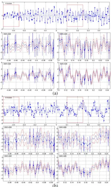
Fig. 3. Top rows: real part of true noise-free function (blue solid) and unequally spaced samples (blue discs) for (subfigure (a)) and mode (sub-figure (b)) case. Second and third rows: Zooms on approximations in the region highlighted in the top rows for and (second and third rows, respectively). True function (blue solid), averaged approxima-tion (black dashed) with 1.96 standard deviaapproxima-tion error tube (red solid), averaged sample values (blue discs) with 1.96 standard deviation error bars (blue solid).
Fig. 4. nRMSE (in dB) of approximations obtained for unequally spaced data for (left column) and exponentials (right column).
example. Similar conclusions are drawn from Fig. 6, plotting the normalized mean squared errors of the approximations: nRMSE values for ESPRIT are consistently roughly 1 dB above those of the proposed method for the regular sampling case and are large for the missing data cases. The dIAA method has large approximation error in all of the three scenarios. We
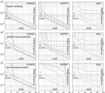
Fig. 5. RMSEs of for exponentials obtained with the proposed method (left column), ESPRIT (center column: standard (solid lines), ES-PRIT-CS (dotted)) and dIAA (right column), respectively; each mode is plotted in a different color. The dashed lines show the square roots of the CRBs. Top row: no missing data. Second row: 100 samples missing at random locations. Bottom row: 2 blocks of 50 missing samples.
have noted that similar results (not reported here for space reasons) are obtained for ESPRIT when applied to interpolated data instead of missing data replaced by zeros, i.e., when mimicking the unequally spaced algorithm rather than using the weighted algorithm. The performance is further illustrated in Fig. 7, where averages and standard deviations of the approximations are plotted together with the true function . Averages and standard deviations of the available samples for are also displayed for the case of two blocks of missing samples. The Hankel ADMM procedure yields good approximations of the true function , including in the zones where no data is available. In contrast, both the ESPRIT and dIAA method yield only rough approximations with large errors. Similar results have been obtained for exponentials and lead to the same conclusions.
E. Model Order Estimation
This section is testing the modified ESTER criterion on the two cases and . The left panel of Fig. 8 shows error bar plots for the criterion in blue
and red for 100 independent noise realizations. For each realization was normalized to have a maximum value of 1, to account for the relative certainty in each simulation. The right panel of Fig. 8 shows histograms of the outcomes of using the modified ESTER criterion for model order selection for the two cases and , respectively. Clearly, the criterion yields excellent model order estimates for large SNR values. For SNR values below 7.5 dB (10 dB) for , the performance of the method degrades. This is consistent with the above results indicating that for low SNR values, the error of the Hankel ADMM based estimates from which the ESTER criterion is computed also increases significantly, see Fig. 2.
Fig. 6. nRMSE (in dB) of approximations obtained for equally spaced data with the proposed Hankel ADMM approach (left column) , ESPRIT (center column; standard (blue circles) and ESPRIT-CS (red crosses)) and dIAA (right column). Top row: no missing data. Second row: 100 samples missing at random locations. Bottom row: 2 blocks of 50 samples missing.
Fig. 7. Top row: real part of true noise-free function (blue solid) and equally spaced samples (blue discs) for exponentials and missing data. Second to fourth row: Zooms on approximations for the regions highlighted in the top rows for . The second row is obtained with the proposed Hankel ADMM based approach, the third row corresponds to ESPRIT, the fourth row to dIAA. True function (blue solid), averaged approximation (black dashed) with 1.96 standard deviation error tube (red solid), averaged sample values (blue discs) with 1.96 standard deviation error bars (blue solid).
F. Convex Relaxation Using Nuclear Norm
This section investigates the potential use of the nuclear norm replacing in the Hankel ADMM based procedure. We con-sider the representative example of unequally spaced samples with for exponentials. Fig. 9 (top left) plots the normalized mean squared errors obtained with the pro-posed method as a function of the augmented parameter (blue,
Fig. 8. Left: Error bar plot of the ESTER model criterion for the two unequally spaced cases ( and in blue and red, respectively). Right: His-togram of model selection outcome using the criterion. The -axis gives the SNR in dB.
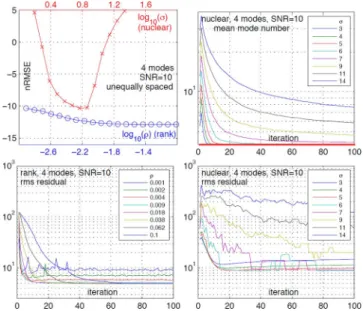
Fig. 9. Top left: nRMSE of approximations obtained with rank constraint (blue, circles) and nuclear norm (red, crosses) as a function of augmented parameter and nuclear parameter , respectively. Top right: averaged number of com-plex exponentials selected by nuclear norm as a function of iteration number for various values of the nuclear parameter . Bottom row: root mean squared distance between the true function and its estimate versus iteration number for rank constraint (left, for various values ) and for nuclear norm (right, for various values of , fixed).
circles) and with nuclear norm as a function of the nuclear norm penalty parameter (red, circles; the augmented parameter is fixed).
Clearly, the proposed method yields solutions that are con-sistently better than those obtained with the nuclear norm for which nRMSE values are more than 2.5 dB higher. This can also be observed in Table IV, where RMSEs of parameters obtained with the rank constraint are compared to those obtained with the nuclear norm with optimal parameter . Moreover, Fig. 9 (top left) indicates that the proposed method is very robust with respect to the precise choice of the tuning parameter . In con-trast, the nuclear norm alternative is very sensitive to the choice of : there exists only a small zone around the “optimal” value
TABLE IV
RMSES OFESTIMATORS AND FOR THEPROPOSEDMETHODWITH
NON-CONVEXRANKCONSTRAINT ANDWITHNUCLEARNORMWITHOPTIMAL
PARAMETER
of for which the performance is reasonable. This renders the selection of difficult while it is at the same time critical since it has a strong impact on the model order selected by the algo-rithm (cf., Fig. 9, top right).
We finally illustrate the convergence of the Hankel ADMM based approach. Root mean squared residuals between the ap-proximations and the true function are plotted in Fig. 9 (bottom) w.r.t. iteration number for rank constraint (bottom left) and nuclear norm (bottom right). For reasonable choices of , the proposed method converges in about iterations.
VI. THETWO-DIMENSIONALCASE
The proposed method is fairly straightforward to generalize to higher dimensions. We will briefly discuss the two-dimen-sional (2D) case and illustrate it with an example. As in the one-dimensional case, there is a relationship between block-Hankel matrices and sums of exponentials. A block Hankel matrix is generated by a sampled function of two variables. Assume that
where the complex frequencies are assumed to be distinct. Consider two sets of equally spaced nodes
and let for
define a 2D sampling of a function as in (4). A block-Hankel matrix can be generated by as follows
. .. . .. .. . . .. . .. ... . .. . .. .. . . .. . .. ...
For the minimization counterparts of (6) and (8) in 2D we simply replace the Hankel matrix by a block-Hankel matrix. The ADMM based methods for obtaining approx-imate solutions based on (9) is easy to generalize using block-Hankel matrices instead of Hankel matrices. We briefly describe the necessary changes in the main algorithm of Table I. The operation now corresponds to the
construction of the block-Hankel matrices above and the operation computes sums over matrices of size according to the Hankel indexing above. For the interpolation matrix , the definition (7) is replaced by a tensor product of one-di-mensional interpolating functions (see, e.g., [59], [60]). The only difficult part in the generalization of the main algorithm in Table I concerns the computation of the modes . If and , it is possible to find the modes using each independent variable separately. For the general case, one can obtain the modes by finding the roots of a system of two polynomials in two variables, as suggested in [61]. This last approach will be used in this paper.
We conclude this section with a simple numerical illustration of the method. We are interested in recovering the function
from 20 quasi-random samples in the box . equals 4 in this example since two exponential functions are as-sociated with each cosine. An example of function and the corresponding samples are shown in Fig. 10. The top panel of the figure shows the function as a transparent surface plot, along with the sampled data indicated by red and blue dots. The color of the dots is related to their sign (blue for positive and red for negative sign, respectively). Moreover, the location in the -plane is depicted with black dots, and blue and red lines that connect the projection onto the -plane with the sam-pled points on the graph of . To further illustrate the 3d-shape, curves connecting each data point with its two closest neighbors (in the -plane) are depicted. The bottom left panel of Fig. 10 shows the same setup but viewed from above.
The bottom middle and right panels show the correct and its reconstruction obtained by the proposed algorithm (viewed as images), using and . The actual and reconstructed images are indistinguishable by eye. The average point-wise error in the reconstruction is 0.0025 (and the max-imum amplitude of is 1). The estimated values of
are given in Table V. This example illustrates the fact that the proposed method can estimate sums of exponentials in two di-mensions.
VII. CONCLUSIONS
We have developed a parametric frequency estimation proce-dure based on approximations with sums of complex expo-nentials. Kronecker’s theorem is used to cast the approximation problem in terms of generating functions for Hankel matrices of rank . The corresponding optimization problem is solved by an ADMM type procedure (using interpolation matrices to accommodate for irregular sampling) allowing an appropriate Hankel matrix to be estimated. The parameters of the complex exponentials associated with the proposed frequency estimation model are then estimated from the solution Hankel matrix. This is in contrast with other methods, such as classical NLS, sub-space methods, or greedy approaches.
The proposed Hankel ADMM based procedure can be ap-plied to irregularly sampled data, as well as to equally spaced samples, including situations with missing data. If available,
Fig. 10. Top panel: 20 quasi-random data samples (red and blue points) of a sum of two 2D cosine functions. For illustration purpose, the underlying func-tion is shown as a surface and each data sample and its two closest neigh-bors are connected by lines o this surface. Bottom panels from left to right: The quasi-random sampling seen from above; the original underlying function; the reconstruction obtained by the proposed algorithm given the 20 unequally spaced samples.
TABLE V
ESTIMATEDVALUES FOR THE2D ESTIMATIONPROBLEM
prior information on the reliability (e.g., noise variance) of data samples can be incorporated using appropriate weighting.
The optimization problem studied in this work is non convex due to the rank constraint on the Hankel matrices. However, nu-merical simulations indicate that the method performs well both for the unequally spaced and regular sampling cases. For suffi-ciently high SNR values, the procedure yields ML parameter estimates, without the need of initializing at a “good” starting point as is crucial for classical NLS in order to avoid local minima. The proposed estimation strategy also consistently out-performs a convex variant in which the rank constraint is re-placed by the nuclear norm. The proposed algorithm is practi-cally attractive due to its simplicity and ease of implementation. The proposed method is also relevant in other contexts, including, e.g., image restoration, source detection and seismic data processing. Future work will also include applications in the context of direction of arrival estimation, extending recent work of the authors on the problem in [62]. In the multidi-mensional case, the proposed method can be relevant, e.g., in
synthetic aperture radar (SAR) [4], [5] where, under suitable assumptions, data acquisition gives rise to unequally spaced Fourier data (e.g., on polar grids), and sampling constraints often induce missing data situations.
ACKNOWLEDGMENT
We are grateful to the authors of [2] which have kindly pro-vided us the original code for dIAA. Part of this work was con-ducted within the Labex CIMI during visits of F. Andersson and M. Carlsson at University of Toulouse.
REFERENCES
[1] P. Stoica and R. Moses, Spectral Analysis of Signals. Englewood Cliffs, NJ, USA: Prentice-Hall, 2005.
[2] E. Gudmundson, P. Stoica, J. Li, A. Jakobsson, M. Rowe, J. Smith, and J. Ling, “Spectral estimation of irregularly sampled exponentially de-caying signals with applications to RF spectroscopy,” J. Magn. Reson., vol. 203, no. 1, pp. 167–176, 2010.
[3] E. Gudmundson, P. Wirfalt, A. Jakobsson, and M. Jansson, “An ES-PRIT-based parameter estimator for spectroscopic data,” in Proc. IEEE
Statist. Signal Process. Workshop (SSP), Ann Arbor, MI, USA, Aug.
2012, pp. 77–80.
[4] M. Cheney, “A mathematical tutorial on synthetic aperture radar,”
SIAM Rev., vol. 43, no. 2, pp. 301–312, 2001.
[5] F. Andersson, R. Moses, and F. Natterer, “Fast Fourier methods for synthetic aperture radar imaging,” IEEE Trans. Aerosp. Electron. Syst., vol. 48, no. 1, pp. 215–229, 2012.
[6] R. J. A. Little and D. B. Rubin, Statistical analysis with missing data, 2nd ed. New York, NY, USA: Wiley, 2002.
[7] R. Kumaresan and D. Tufts, “Estimating the parameters of exponen-tially damped sinusoids and pole-zero modeling in noise,” IEEE Trans.
Signal Process., vol. 30, no. 6, pp. 833–840, 1982.
[8] D. Tufts and R. Kumaresan, “Estimation of frequencies of multiple si-nusoids: Making linear prediction perform like maximum likelihood,”
Proc. IEEE, vol. 70, no. 9, pp. 975–989, 1982.
[9] P. Stoica, R. Moses, B. Friedlander, and T. Söderström, “Maximum likelihood estimation of the parameters of multiple sinusoids from noisy measurements,” IEEE Trans. Acoust., Speech, Signal Process., vol. 37, no. 3, pp. 378–392, 1989.
[10] M. Macleod, “Fast nearly ML estimation of the parameters of real or complex single tones or resolved multiple tones,” IEEE Trans. Signal
Process., vol. 46, no. 1, pp. 141–148, 1998.
[11] Y. Li, K. J. R. Liu, and J. Razavilar, “A parameter estimation scheme for damped sinusoidal signals based on low-rank Hankel approxima-tion,” IEEE Trans. Signal Process., vol. 45, no. 2, pp. 481–486, 1998. [12] B. Quinn and E. Hannan, The Estimation and Tracking of Frequency, ser. Statistical And Probabilistic Mathematics. Cambridge, U.K.: Cambridge Univ. Press, 2001.
[13] P. Babu and P. Stoica, “Spectral analysis of nonuniformly sampled data—a review,” Digit. Signal Process., vol. 20, no. 2, pp. 359–378, 2010.
[14] R. Schmidt, “Multiple emitter location and signal parameter estima-tion,” IEEE Trans. Antennas Propag., vol. 34, no. 3, pp. 276–280, 1986. [15] R. Roy and T. Kailath, “ESPRIT-estimation of signal parameters via rotational invariance techniques,” IEEE Trans. Acoust., Speech, Signal
Process., vol. 37, no. 7, pp. 984–995, 1989.
[16] R. Kumaresan and D. W. Tufts, “Estimating the angles of arrival of multiple plane waves,” IEEE Trans. Aerosp. Electron. Syst., vol. 19, no. 1, pp. 134–139, 1983.
[17] H. Clergeot, S. Tressens, and A. Ouamri, “Performance of high res-olution frequencies estimation methods compared to the Cramer-Rao bounds,” IEEE Trans. Acoust., Speech, Signal Process., vol. 37, no. 11, pp. 1703–1720, 1989.
[18] P. Stoica and A. Nehorai, “Music, maximum likelihood and Cramér-Rao bound,” IEEE Trans. Acoust., Speech, Signal Process., vol. 37, no. 5, pp. 720–741, 1989.
[19] P. Stoica and A. Nehorai, “Music, maximum likelihood and Cramér-Rao bound: further results and comparisons,” IEEE Trans.
Acoust., Speech, Signal Process., vol. 38, no. 12, pp. 2140–2150,
1990.
[20] P. Stoica and T. Söderström, “Statistical analysis of MUSIC and sub-space rotation estimates of sinusoidal frequencies,” IEEE Trans. Signal
Process., vol. 39, no. 8, pp. 1836–1847, 1991.
[21] C. Rao and L. Zhao, “Asymptotic behavior of maximum likelihood estimates of superimposed exponential signals,” IEEE Trans. Signal
Process., vol. 41, no. 3, pp. 1461–1464, 1993.
[22] T.-H. Li and K.-S. Song, “On asymptotic normality of nonlinear least squares for sinusoidal parameter estimation,” IEEE Trans. Signal
Process., vol. 56, no. 9, pp. 4511–4515, 2008.
[23] T.-H. Li and K.-S. Song, “Estimation of the parameters of sinusoidal signals in non-Gaussian noise,” IEEE Trans. Signal Process., vol. 57, no. 1, pp. 62–72, 2009.
[24] C. Rao, L. Zhao, and B. Zhou, “Maximum likelihood estimation of 2-d superimposed exponential signals,” IEEE Trans. Signal Process., vol. 42, no. 7, pp. 1795–1802, 1994.
[25] Y. Bresler and A. Macovski, “Exact maximum likelihood parameter estimation of superimposed exponential signals in noise,” IEEE Trans.
Acoust., Speech, Signal Process., vol. 34, no. 5, pp. 1081–1089, 1986.
[26] G.-O. Glentis and A. Jakobsson, “Efficient implementation of iterative adaptive approach spectral estimation techniques,” IEEE Trans. Signal
Process., vol. 59, no. 9, pp. 4154–4167, 2011.
[27] G.-O. Glentis and A. Jakobsson, “Superfast approximative implemen-tation of the IAA spectral estimate,” IEEE Trans. Signal Process., vol. 60, no. 1, pp. 472–478, 2012.
[28] S. Bourguignon, H. Carfantan, and J. Idier, “A sparsity-based method for the estimation of spectral lines from irregularly sampled data,”
IEEE J. Sel. Topics Signal Process., vol. 1, no. 4, pp. 575–585, 2007.
[29] P. Stoica, P. Babu, and L. Jian, “New method of sparse parameter es-timation in separable models and its use for spectral analysis of irreg-ularly sampled data,” IEEE Trans. Signal Process., vol. 59, no. 1, pp. 35–47, 2011.
[30] M. Duarte and R. Baraniuk, “Spectral compressive sensing,” Appl.
Comput. Harmon. Anal., vol. 35, no. 1, pp. 111–129, 2013.
[31] P. R. Stoica and P. Babu, “Sparse estimation of spectral lines: Grid selection problems and their solutions,” IEEE Trans. Signal Process., vol. 60, no. 2, pp. 962–967, 2012.
[32] N. Lomb, “Least-squares frequency analysis of unequally spaced data,”
Astrophys. Space Sci., vol. 39, no. 2, pp. 447–462, 1976.
[33] J. Scargle, “Studies in astronomical time series analysis. II-statistical aspects of spectral analysis of unevenly spaced data,” Astrophys. J., vol. 263, pp. 835–853, 1982.
[34] W. Press and G. Rybicki, “Fast algorithm for spectral analysis of un-evenly sampled data,” Astrophys. J., vol. 338, no. 1, pp. 277–280, 1989. [35] M. Schulz and K. Stattegger, “Spectrum: Spectral analysis of unevenly spaced paleoclimatic time series,” Comput. Geosci., vol. 23, no. 9, pp. 929–945, 1997.
[36] V. Adamjan, D. Arov, and M. Krein, “Infinite Hankel matrices and gen-eralized problems of Carathéodory-Fejér and F. Riesz,” Funkcional.
Anal. i Prilozen., vol. 2, no. 1, pp. 1–19, 1968.
[37] F. Andersson, M. Carlsson, and M. d. Hoop, “Sparse approximation of functions using sums of exponentials and AAK theory,” J. Approx.
Theory, vol. 163, no. 2, pp. 213–248, Feb. 2011.
[38] R. Rochberg, “Toeplitz and Hankel operators on the Paley-Wiener space,” Integral Eq. Operator Theory, vol. 10, no. 2, pp. 187–235, 1987.
[39] F. Andersson and M. Carlsson, “Alternating projections on non-tan-gential manifolds,” Constr. Approx., vol. 38, no. 3, pp. 489–525, 2013. [40] G. Beylkin and L. Monzon, “On approximation of functions by expo-nential sums,” Appl. Comput. Harmon. Anal., vol. 19, no. 1, pp. 17–48, Jul. 2005.
[41] F. Andersson, M. Carlsson, J.-Y. Tourneret, and H. Wendt, “Frequency estimation based on Hankel matrices and the alternating direction method of multipliers,” presented at the Eur. Signal Process. Conf. (EUSIPCO), Marrakech, Morocco, Sep. 2013.
[42] I. Markovksy, Low Rank Approximation: Algorithms, Implementation,
Applications. New York, NY, USA: Springer, 2012.
[43] L. Condat and A. Hirabayashi, “Robust spike train recovery from noisy data by structured low rank approximation,” presented at the Int. Conf. Sampl. Theory Appl. (SAMPTA), Bremen, Germany, Jul. 2013.
[44] L. Condat, J. Boulanger, N. Pustelnik, S. Sahnoun, and L. Seng-manivong, “A 2-d spectral analysis method to estimate the modulation parameters in structured illumination microscopy,” presented at the IEEE Int. Symp. Biomed. Imag. (ISBI), Beijing, China, Apr. 2014. [45] L. Condat and A. Hirabayashi, “Cadzow denoising upgraded: A
new projection method for the recovery of Dirac pulses from noisy linear measurements,” Sampl. Theory Signal Image Process., 2014 [Online]. Available: http://hal.archives-ouvertes.fr/docs/00/84/79/84/ PDF/double.pdf, to be published
[46] E. Candès and C. Frenandez-Granda, “Towards a mathematical theory of super-resolution,” Comm. Pure Appl. Math, 2013 [Online]. Avail-able: http://dx.doi.org/10.1002/cpa.21455
[47] Super-Resolution Imaging, ser. Digital Imaging and Computer Vision, P. Milanfar, Ed. Princeton, NJ, USA: Princeton Univ. Press, 2010. [48] S. Boyd, N. Parikh, E. Chu, B. Peleato, and J. Eckstein, “Distributed
op-timization and statistical learning via the alternating direction method of multipliers,” Found. Trends Mach. Learn., vol. 3, no. 1, pp. 1–122, 2011.
[49] M. Fazel, T. K. Pong, D. Sun, and P. Tseng, “Hankel matrix rank min-imization with applications to system identification and realization,”
SIAM J. Matrix Anal. Appl., vol. 34, no. 3, pp. 946–977, 2013.
[50] C. Jian-Feng, E. Candès, and S. Zuowei, “A singular value thresholding algorithm for matrix completion,” SIAM J. Optim., vol. 20, no. 4, pp. 1956–1982, 2010.
[51] D. Slepian and H. O. Pollak, “Prolate spheroidal wave functions, Fourier analysis and uncertainty,” Bell Syst. Tech. J., vol. 40, no. 1, pp. 43–63, 1961.
[52] G. Strang and G. Fix, “A Fourier analysis of the finite element varia-tional method,” in Constructive Aspects of Funcvaria-tional Analysis. New York, NY, USA: Springer, 2011, pp. 793–840.
[53] R. Keys, “Cubic convolution interpolation for digital image pro-cessing,” IEEE Trans. Acoust., Speech, Signal Process., vol. 29, no. 6, pp. 1153–1160, 1981.
[54] I. German, “Short kernel fifth-order interpolation,” IEEE Trans. Signal
Process., vol. 45, no. 5, pp. 1355–1359, 1997.
[55] R. Charpentier, “Nonconvex splitting for regularized low-rank + sparse decomposition,” IEEE Trans. Signal Process., vol. 60, no. 11, pp. 35–47, 2012.
[56] R. Badeau, B. David, and G. Richard, “Selecting the modeling order for the esprit high resolution method: An alternative approach,” in Proc.
IEEE Int. Conf. Acoust., Speech, Signal Process. (ICASSP), 2004, vol.
2, pp. 1025–1028.
[57] R. Horn and C. Johnson, Topics in matrix analysis. Cambridge, U.K.: Cambridge Univ. Press, 1994.
[58] M. Haardt and J. A. Nossek, “Unitary esprit: How to obtain increased estimation accuracy with a reduced computational burden,” IEEE
Trans. Signal Process., vol. 43, no. 5, pp. 1232–1242, 1995.
[59] L. D. Lathauwer, B. D. Moor, and J. Vandewalle, “On the best rank-1 and rank-(r 1, r 2,..., rn) approximation of higher-order tensors,” SIAM
J. Matrix Anal. Appl., vol. 21, no. 4, pp. 1324–1342, 2000.
[60] J.-M. Papy, L. D. Lathauwer, and S. V. Huffel, “Exponential data fitting using multilinear algebra: the decimative case,” J. Chemometrics, vol. 23, pp. 341–351, 2009.
[61] F. Andersson, M. Carlsson, and M. V. D. Hoop, “Nonlinear approxima-tion of funcapproxima-tions in two dimensions by sums of exponential funcapproxima-tions,”
Appl. Comput. Harmon. Anal., vol. 29, no. 2, pp. 156–181, 2010.
[62] F. Andersson, M. Carlsson, J.-Y. Tourneret, and H. Wendt, “On an iter-ative method for direction of arrival estimation using multiple frequen-cies,” presented at the IEEE Int. Workshop Comput. Adv. Multi-Sensor Adapt. Process. (CAMSAP), Saint-Martin, France, Dec. 2013.
Fredrik Andersson received his M.Sc. in
engi-neering physics (2000) and Ph.D. in mathematics (2005) from Lund University, Sweden. He is cur-rently working as associate professor at the Centre for Mathematical Sciences at Lund University. His research interests include fast algorithms, inverse problems and approximation theory. During 2013, he was participating as a scientific expert in the CIMI thematic trimester on Image Processing at the University of Toulouse.
Marcus Carlsson received his M.Sc. degree in
Mathematics in 2002, and his Ph.D. degree in Math-ematics in 2007, both from Lund University, Lund, Sweden. From 2007 to 2010, he was a Research Associate Professor with the Department of Math-ematics and with the Geo-Mathematical Imaging Group at Purdue University, Indiana, USA. In 2011, he worked as Research Professor at the Department of Mathematics at Universidad de Santiago de Chile. Since 2012, he has held a tenure track research position at the Centre for Mathematical Sciences at Lund University.
Jean-Yves Tourneret (SM’08) received the
In-génieur degree in electrical engineering from the Ecole Nationale Supérieure d’Electronique, d’Elec-trotechnique, d’Informatique, d’Hydraulique et des Télécommunications (ENSEEIHT) de Toulouse in 1989 and the Ph.D. degree from the National Polytechnic Institute from Toulouse in 1992. He is currently a professor in the University of Toulouse (ENSEEIHT) and a member of the IRIT laboratory (UMR 5505 of the CNRS). His research activities are centered around statistical signal and image pro-cessing with a particular interest to Bayesian and Markov chain Monte Carlo (MCMC) methods. He has been involved in the organization of several confer-ences including the European conference on signal processing EUSIPCO’02 (program chair), the international conference ICASSP’06 (plenaries), the statistical signal processing workshop SSP’12 (international liaisons), the International Workshop on Computational Advances in Multi-Sensor Adaptive Processing CAMSAP 2013 (local arrangement), and the statistical signal pro-cessing workshop SSP’2014 (special sessions). He has been the general chair of the CIMI workshop on optimization and statistics in image processing hold in Toulouse in 2013. He has been a member of different technical committees including the Signal Processing Theory and Methods (SPTM) committee of the IEEE Signal Processing Society (2001–2007, 2010–present). He has been serving as an associate editor for the IEEE TRANSACTIONS ONSIGNAL
PROCESSING(2008–2011) and for the EURASIP Journal on Signal Processing (since July 2013).
Herwig Wendt (M’13) received the M.S. degree
in electrical engineering and telecommunications from Vienna University of Technology, Austria, in 2005. In September 2008, he received the Ph.D. degree in Physics and Signal processing from Ecole Normale Supérieure de Lyon. From October 2008 to December 2011, he was a Postdoctoral Research Associate with the Department of Mathematics and with the Geomathematical Imaging Group, Purdue University, West Lafayette, Indiana. Since 2012, he is a permanent researcher of the Centre National de Recherche Scientifique (CNRS) within the Signal and Communicatons Group of the Institut de Recherche en Informatique de Toulouse (IRIT) of the University of Toulouse.