To link to this article :
URL :
http://www.publishresearch.com/download/1303
To cite this version :
Mnasri, Sami and Van den Bossche, Adrien and
Nasri, Nejah and Val, Thierry The 3D Deployment Multi-objective
Problem in Mobile WSN: Optimizing Coverage and Localization.
(2015) International Research Journal of Innovative Engineering -
IRJIE, vol. 1 (n° 5). ISSN 2395-0560
O
pen
A
rchive
T
OULOUSE
A
rchive
O
uverte (
OATAO
)
OATAO is an open access repository that collects the work of Toulouse researchers and
makes it freely available over the web where possible.
This is an author-deposited version published in :
http://oatao.univ-toulouse.fr/
Eprints ID : 15315
Any correspondence concerning this service should be sent to the repository
administrator:
[email protected]
The 3D Deployment Multi-objective Problem in Mobile
WSN: Optimizing Coverage and Localization
Sami Mnasri 1, Adrien van den Bossche2, Nejah Narsi3, Thierry Val4
1
University of Toulouse, UT2J, CNRS-IRIT-IRT, Toulouse, 31058, France
2
University of Toulouse, UT2J, CNRS-IRIT-IRT, Toulouse, 31058, France
3
University of Sfax, ENIS,LETI, Sfax, 3038, Tunisia
4
University of Toulouse, UT2J, CNRS-IRIT-IRT, Toulouse, 31058, France
Abstract
The deployment of sensor nodes is a critical phase that significantly affects the functioning and performance of the sensor network. Coverage is an important metric reflecting how well the region of interest is monitored. Random deployment is the simplest way to deploy sensor nodes but may cause unbalanced deployment and therefore, we need a more intelligent way for sensor deployment. In this paper, we study the positioning of sensor nodes in a WSN in order to maximize the coverage problem and to optimize the localization. First, the problem of deployment is introduced, then we present the latest research works about the different proposed methods. Also, we propose a mathematical formulation and a genetic based approach to solve this problem. Finally, the numerical results of experimentations are presented and discussed. Indeed, this paper presents a genetic algorithm which aims at searching for an optimal or near optimal solution to the coverage holes problem. Our algorithm defines the mini-mum number and the best locations of the mobile nodes to add after the initial random deployment of the stationary nodes. Com-pared with random deployment, our genetic algorithm shows significant performance improvement in terms of quality of cover-age while optimizing the localization in the sensor network.Keywords
Target Coverage, Localization, Mobile Node, 3D Deployment, Genetic Algorithm, NSGAII.1. Introduction
WSNs are generally used in all applications having specific monitoring needs like smart buildings, environmental or military applications …etc.). The efficiency of a wireless sensor network is greatly influenced by the process of deploying and positioning the sensor nodes. In a WSN, the deployment of sensor nodes is a strategy that aims to define the number of the sensor nodes, its positions and the topology of the network. Different issues are discussed during the deployment of sensor nodes in a WSN.
The sensor node deployment depends also on the application. Indeed, there are some applications where it is possible to select the sites where to place the sensor nodes. This type of deployment is called deterministic. Whereas in some other applications, we simply scatter a large number of nodes over the monitoring region from a plane or a helicopter. This type of deployment is called nondeterministic or random. Deterministic deployment is preferred in amicable environments and it requires fewer sensors than the random deployment. Although, random deployment is usually preferred in large scale sensor networks due to its facility and cheapness and because it might be the only choice in some hostile and remote environments. Generally, the deterministic de-ployment is used when it is expensive to deploy nodes or when their operation is significantly affected by their positions, for in-stance, for target tracking, surveillance or intrusion detection. Even for random deployment case, we can add, in a controlled way, some nodes, to improve the quality of the deployment. For all these reasons, our paper is focused on deterministic deployment. The coverage is the global objective and the most important to satisfy during the deployment of a WSN. It is an essential topic in the design of a WSN and one of the most active fields of research in this domain. The coverage is generally interpreted as the way in which a network of sensors will supervise the area of interest. The coverage can be considered as a measurement of the quality of service and the reliability of the network. The coverage can be measured in various manners according to the application. In order to increase the area of coverage, a set of redundant sensors are deployed. The redundancy of nodes increases the density of the wireless sensor networks compared to the normal ad hoc networks. However, increasing the number of sensors cannot provide
a 100% probability of coverage, it also expensive to maintain networks with high density on a large scale. Consequently, other approaches must be applied in order to avoid these problems and to improve the coverage after the random initial deployment.
Generally, the considered coverage problems are either area coverage, target cover (point coverage), coverage with optimiza-tion of power consumpoptimiza-tion, or K-coverage problem. Coverage area can be defined, according to [1], as: "the area in which a sen-sor can perform its sensing, monitoring, surveillance and detection tasks with a reasonable accuracy (i.e., the sensen-sor reading have at least a threshold level of sensing detection probabilities within the area). The target coverage (called also point coverage) inter-est in controlling a target in the field of interinter-est that can be stationary or mobile. The k-coverage problem requires preserving at least k sensor nodes controlling any target to consider it covered.
The localization of the sensors is the most significant factor related to the cover network. Localization is important when there is an uncertainty of the exact position of some nodes. Indeed, in wireless sensor networks, the location information is crucial es-pecially when an unusual event occurs. In this case, sensor node that detected that event needs to locate it and then report this po-sition to the base station. Considering works done, we propose in our paper a model for optimal sink nodes deployment in WSN. We propose two objective functions: The network coverage and the localization. For most deployment formulations, the prob-lem of optimal placement of the sensor nodes is proven NP-hard [2]. Consequently, for large scale instances, this probprob-lem cannot be solved by deterministic methods such as the circle packing algorithm. We define the problem formally and we propose an effi-cient genetic algorithm to resolve the problem of the coverage holes after the initial random deployment. For a given number of sensors, the proposed algorithm attempts to maximize the sensor field coverage using a set of operators. In our works, we are in-teresting in using WSN in smart buildings applications. Despite the different challenges in WSNs, research works have only fo-cused on post-deployment problems such as: sensors localization, MAC efficiency or routing optimization, etc. Our works aim to ensure the deployment of the nodes while maximizing the coverage and optimizing the localization using an efficient genetic al-gorithm. Our proposed model is different from the existing models since it integrates sensor node deployment, and localization approach in a single model.
The rest of the paper is organized as follows: In Section II, the related works are presented. In Section III, a mathematical mod-elling is proposed. In Section IV, the used 3D target localization algorithm is explained. In section V, the genetic algorithm based approach is explained. In Section VI, experimental results are presented. In section VII, a discussion is established, and finally, the section VIII concludes the paper.
2. Related Works
Many recent researches propose evolutionary approaches like genetic algorithms to ensure an efficient deployment model in WSN. In [3], [4], [5], [6] and [7], authors interests in studying the sensor deployment problems. Also, in [8], the coverage prob-lem is studied in the domain of the robot exploration. This work considers each robot as a sensor node and the used algorithm deploy nodes one by one incrementally. Hence, the proposed algorithm is computationally expensive, when we increase the num-ber of nodes. Among the recent researches proposing genetic algorithms to ensure an efficient deployment model in the WSN, we present the following works. The works of [9] propose a multi-objective paradigm to solve the deployment and power assignment problem. This evolutionary algorithm is based on multi objective evolutionary algorithm with decomposition. According to their numerical results, their algorithm is better than the NSGAII for different instances. Also, the works of [10] present a genetic algo-rithm that aims to solve the problem of coverage holes. The proposed algoalgo-rithm determines the minimum number and the best locations of mobile nodes to add after the initial deployment of stationary nodes. The study in [11] aims to propose different multi-objective methodologies to resolve the problem of sensor deployment in order to optimize the coverage, the connectivity, the cost and the lifetime. Author’s presents different studies based on genetic algorithms and particle swarms. The works of [12] study the problem of redeployment and different algorithms are developed to maximize the detection range and to minimize the energy consumption. Two centralized optimization algorithms are developed; one is based on the genetic algorithms and the other is based on particle swarm optimization. The genetic algorithm is used to determine the optimal trade-off between the ratio of network coverage and the overall distance travelled by the mobile nodes with a fixed radius of detection. Concerning the spatial localization and the adaptive beacon placement, the works of [13] propose different techniques for both coarse-grained and fine-grained localization. The study of [14] discusses the problem of evaluating the coverage after deployment and the self-localization of mobile nodes. It proposed a polynomial algorithm that uses computational geometry and graph theory to de-fine the best-case and the worst-case coverage.
3. Mathematical Formulation
We present the following model to resolve our problem. The objective is to provide a deployment scheme while optimizing the target coverage of the localization. To best locate, we aim to optimize the placement of nodes with the most possible uniform dis-tribution of nodes (anchors and mobile nodes) around the target to locate. Among the considered constraints, the non-alignment of
nodes and a well-studied distances between them. The set of targets to detect; the location of potential sites to install the sensors; the transmission power, the cost and the minimum number of received signals to detect a target are considered known in our model.
3.1 Assumptions
We set the following assumptions:
- The anchor node can be a sensor placed in a specific location, a nomad sensor or a sensor attached to a mobile target. - In the case of the k-coverage, the located target must be within the range of at least k anchors nodes.
- According to the used 3D localization scheme based on DVHop and RSSI measurements (which will be explained in the next section), we suppose that we use four anchors to locate each target.
- We suppose that rooms and halls have heterogeneous 3D spaces.
3.2 Notation
The following notation is used in this paper. It is composed of sets, decision variables and parameters. • Sets
ü T: set of targets to detect in the field, tk is a target.
ü N: the set of different types of sensor nodes, N = Na
∪
Nb.Na, the set of different types of stationary nodes Nb the set of different types of mobile nodes
ü S: set of potential sites to install the sensor nodes S = Sa
∪
SbSa the set of potential sites to install the stationary sensor nodes, na is a site of a stationary node. Sb the set of potential sites to install the mobile sensor nodes, nm is a site of a mobile node.
(a site may not be in both sets, that is, Sa
∩
Sb ≠∅
) • Decision Variablesü
n s
W
be a 0-1 variable such that
n s
W
= 1 if and only if a node of type n ∈ N is installed at site s
∈
Sü Xts, a 0-1 variable such that Xts = 1 if the node of type n
∈
N installed at site s∈
S receives a signal from a target atthe position t
∈
T with a power greater than or equal to the minimum required power by the node to detect it. üSg
ss' is also a 0-1 variable such thatSg
ss' = 1 if and only if the node installed at site s∈
S receives a signal froman-other node installed at site s'
∈
S with a power greater than or equal to the minimum required. ü ' ' nn ssSg
, be a 0-1 variable such that
' ' nn ss
Sg
= 1 if and only if the node of type n
∈
N installed at site s∈
S receives a signal from another node of type n'∈
N installed at site s' ∈ S with a power greater than or equal to the minimum re-quired power.ü Ms is the minimum number of hops between a stationary node installed at site s
∈
S to any mobile node. • Parametersü
γ
ts be the signal attenuation ratio from the target t∈
T to site s∈
S,ü
δ
ss' the attenuation ratio between the sites s∈
S and s'∈
S,ü Pt is the transmission power of a target at the position t
∈
T (in watts).ü pn is the transmission power of a node of type n
∈
N (in watts). ü minn
P
is the minimum power of a received signal by a node of type n
∈
N to detect it (i.e. the sensibility). ü nmin the minimum number of nodes receiving a signal from a target to localize it (in our case, nmin∈
{2,3}),ü hpmax, the maximum number of hops between an anchor node and a mobile node,
ü cs the cost of a node of type n
∈
N and installing it at site s∈
S.ü
1 2 m m ij
Ag
Angle between two sensors m1 and m2 of two different and adjacent nodes i and j. ü n: length of the RoI (Region of interest).
ü m: width of the RoI
ü r: radius of a sensor (all the sensor nodes have the same sensing range). ü nbNa: number of stationary nodes
ü nbNm: number of mobile nodes needed to add. ü nbT: number of targets
ü Sgij : power of the signal transmitted between two nodes i and j.
ü dij : distance between two nodes i and j,
ü dm1m2: a constant representing the distance between two sensors.
ü dmax: a constant representing the maximum distance between two nodes i and j (or a node i and a target j) so that they can
be detectable.
3.3 Objective function
To model the problem of target coverage considering the localization, we consider the following objective function.
• Coverage: Let F1 be the fitness of a mobile node i (nmi) which calculates the coverage as a function of the targets it cov-ered, we obtain the following function F1 for the coverage
F1= Maximize (
(
)
m m n N mF
n
∈∑
) (1)• Localization: each target must be monitored by at least nmin nodes (mobile or anchor), thus:
min ts s S
x
n
t
T
∈≥
∀ ∈
∑
, we obtain the following function F2 for the localization:F2= Maximize (
(
t s m i n)
t T s S
x
n
+∈ ∈
−
∑ ∑
) knowing that (x)+ = max(0,x) (2)Thus, the fitness function is given by:
F = F1 + F2 =Maximize
(
t s m i n)
(
m)
t T s S n Nx
n
+F
n
∈ ∈ ∈−
+
∑ ∑
∑
(3) 3.4 Constraints F is subject to: min ts s Sx
n
t
T
∈≥
∀ ∈
∑
(4) 1 2 min1
m m/
,
ts tsSg
= ⇒
Ag
= Π
k
n
t
≠
s
(5)[
]
1 21
m m0.
,
ts ts n NSg
Ag
k
t
s
∈= ⇒
∑
∈
Π
≠
(6) 2 min.(
/ 2
)
nbNa
=
n
nm
Π
r
(7).
. (
),
ts ts tsd
=
α
Sg g Sg
α
∈
R
(8) max(
Sg
ts=
1)
⇒
(
d
ts≤
d
)
(9) n ts s s S n Nx
W
∈ ∈≤
∑
∑
(10)' ' ' ' ' min ' ' ' n nn n nn ss ss ss n N n N n N n N
P
Sg
P
Sg
δ
∈ ∈ ∈ ∈≥
∑ ∑
∑
∑
(11) ' ' ' ' nn ss ss n N n NSg
Sg
∈ ∈=
∑ ∑
(12) min, t
T, s
S
n n ts t s n NP
P W
δ
∈≥
∑
∀ ∈
∈
(13)The objective function (3) of the problem aims to optimize the target coverage and the localization. Constraint (4) impose that the number of nodes receiving a signal from the target i must be greater than or equal to the minimum necessary to localize it.
Constraint (5) force the angles of arrival between sensors to be 90° in the case of 2-coverage (nmin=2) and to be 60° in the case of
3-coverage (nmin =3). Constraint (6) concerns the non-linearity of the adjacent nodes in order to optimize the localization.
Con-straint (7) imposes the number of the anchors deployed initially. ConCon-straint (8) link the distance and the power transmission of the
signal between two nodes. g is a function,
α
is real coefficient. Constraint (9), imply that if there is a signal Sgts between two nodes, the distance between these two nodes (dij) should not exceed a fixed maximum distance (dmax). Constraint (10), impose thata target cannot be detected by a number of nodes that exceeds the number of installed nodes in the different sites. Constraint (11) impose that if the node s’ is detected by the node s, then the power transmission resulting from s towards s’ must be higher than the minimum necessary power transmission so that s is detectable by s’. Constraint (12) concerns the power transmission emitted by the node s and received by the node s’, for different types of nodes. Constraint (13) indicate that the node installed at site s must receive a signal from a target at position t with a power greater than or equal to the minimum required to detect it.
4. The Hybrid 3D Target Localization Algorithm
The most existing localization schemes focus only on 2D plane. Although 3D localization is more realistic and accurate. Such as the 2D localization, we distinguish two types of localization in 3D environment: range free localization and the range-based localization. This classification is based on whether the actual distance between nodes must be measured or not. The 3D range-based localization algorithms measure the exact orientation and distance between neighbor nodes, and use the information to localize nodes. However, 3D range-based localization algorithms has some exigency on hardware requirements. Hence, they are more costly to implement in practice. Landscape 3D [15] is a 3D range-based localization algorithm. The 3D Range-free algo-rithms use an estimated distance between nodes to localize them. They reduces the cost of deploying hardware but at the expense of a low 3D localization accuracy [16]. Different 3D Range-free localization algorithms exists as 3DDVHOP algorithm [17], 3Dcentroid algorithm [18] and the 3D multidimensional scaling-map (3D MDS-MAP) [19] which are inspired from 2D plane scenarios.
In order to compensate the deficiency of both algorithms, we propose a hybrid localization method based on combining the hop distance and the RSSI data for 3D WSN localization. We propose a hybrid localization scheme that improves the used range-free technique (DV-HOP) by introducing a RSSI data to revise the hop distance. First, the 3D DV-HOP uses the network connectivity information’s to estimate the node locations in the 3D space. Then, the RSSI value can be easily collected to correct the position of the nodes found by the DV-HOP according to the signal strength. The RSSI value is measured in both directions: starting from the mobile node, we measure the RSSI value received from the other nodes (fixed or mobile); and starting from each fixed or mobile node, we measure the RSSI value received from the mobile node. The final admitted value of the RSSI between the mobile node and each other node is the higher value of the two already mentioned values.
5. The Proposed Genetic Algorithm (NSGA II)
In this section, we present the suggested approach. We present the assumptions of the network, the coverage model, and we dis-cuss the approach based on the genetic algorithm. We aim at maximizing the coverage rate by reducing the holes, and maximizing the localization.. Assuming that Si is the stationary sensor nodes deployed randomly over the region of interest, r is the sensing range of the sensors. The proposed genetic algorithm starts with an initial random population (the distribution of the initial nodes). Then, the objective function evaluates in each iteration the constraints satisfaction rate. The new solution (population) is improved after each iteration of the algorithm. This improvement is carried out through the operators (crossover and mutation). A stopping criterion is used to stop the execution of the algorithm. Indeed, the algorithm starts by initializing the length and the width of the area, the number of stationary sensor nodes, the number of targets, the chromosomes and the random locations of the chromosomes. First, we calculate the coverage ratio of stationary nodes. Then, while the did not reach the required fitness or the maximum number
of iteration, we evaluate the fitness of the chromosome, rank the chromosomes and compute the fitness, do a crossover and mutation on chromosomes, update the value of the chromosomes, and evolve the next generation of the chromosomes. The genetic algorithm is run by the base station after gathering the positions of the stationary nodes in order to determine the number and positions of the mobile nodes as follow:
5.1 Representing a Chromosome
In the proposed genetic algorithm a chromosome represents a solution that indicates the position (location) of a potential mobile node in the region of interest (RoI). This position is modeled as an (X, Y, Z) point. The different gens of the chromosome represent a binary digit that resembles the value of the position on the X and Y axises. For example, to represent a mobile node mapped to the location (50, 65, 42), the corresponding chromosome is shown in Figure 1. The Choice of the size of the chromosome population is based on two factors: the area of the RoI and the initial configuration of the network. For instance, if the radius of each node is 48m and the area of the sensing field is 70 m * 80 m* 120 m, the number of deployed stationary nodes will be (i.e.; (70*80*120)/(4*π*92) ≈ 661), then the algorithm will start with population of 661 randomly generated chromosomes to ensure the full coverage. The value 117 is selected based on the assumption that 661 sensor nodes would cover the entire field as if they were deterministically deployed. If we aim to ensure a k-coverage (each target must be covered by at least k sensor nodes), we have to start with 661 * k chromosomes as an initial population.
X-position Y-position Z-position
1 1 0 0 1 0 1 0 0 0 0 1 1 0 1 0 1 0 Figure1. Chromosome representing the sensor position (50, 65,42)
5.2 Evaluation
After the initialization, each chromosome fitness (i.e.; the goodness of the solution) is evaluated using the fitness function. The fitness or the formulation of the objective depends on characteristics of the problem. The fitness function is used to choose the best fittest chromosomes to reproduce the next generated solutions by the algorithm. The fitness function calculates the maximum number of the covered targets by each mobile node. The overlapping redundancy is prevented by the fitness function among the coverage regions of the deployed mobile nodes. The fitness function is given by:
F = Maximize (
(
ts min)
t T s Sx
n
+ ∈ ∈−
∑ ∑
+(
m)
n NF n
∈∑
) (14) 5.3 ReproductionReproduction is composed of four steps: selection, cross- over, mutation, and accepting the solution. The fitness is used as a measure to rank the chromosomes and to perform parent selection according to the ratio participated by each chromosome in the fitness function in order to reproduce new solutions. However, less fitness members will have also a chance to be selected. Different mechanisms are used to implement the selection step such as the rollet wheel method. The selection will be performed on two chromosomes to reproduce two new chromosomes each time. After selecting the chromosomes, a crossover operation is performed between a pair of parent chromosomes by selecting a random point in chromosomes and exchanging genes after this point. We choose two random crossing points. The child inherits elements positionned between the two crossover points of the first parent. These elements occupy the same positions, and appear in the same order in the child. The selection and crossover operations may lead to a set of identical chromosomes and the algorithm stops creating new individuals. This may prevent the average fitness improvement and thus trapping into a local optimum. To avoid this problem, a mutation operation is applied where a gene is selected randomly and its value is changed. Mutation performs a larger exploration of the search space, to avoid the premature convergence or the disappearance of the diversity while bringing innovation to the population. The mutation is carried out by reversing the position of two genes. Often, each gene is represented by a bit; the mutation is done by flipping a bit randomly in the chromosome. After crossover and mutation, two new chromosomes are reproduced. Finally, if they are better than their parents, they will be accepted as a new population.
5.4 Stopping Criterion
The stopping criterion is either reaching a maximum number of iterations; either reaching a predefined localization rate (if a rate of k-coverage is ensured, k= nmin). Also, we can use a maximum execution time of the algorithm as a stopping criterion.
6. Experimental Results
In this section, we aim at testing our contributions in reality on a set of testbeds by deploying nodes in the IUT of blagnac in Toulouse.
6.1 Environment
- We used the testbed Open Wino (Open Wireless Node) [20] which is a free platform (free hardware and software architecture) for emulation and rapid prototyping of protocols for wireless sensor networks, developed at the IUT of Blagnac and the IRIT la-boratory. The network nodes are based on components from the ecosystem.
- Arduino whichis a hardware and software programming platform allowing the rapid prototyping modules. It is a free Java application used as a code editor and a compiler. It can transfer the firmware and the program through serial links (USB). It has an input /output interface to build independent interactive objects. The Wino nodes are specifically based on processors. We use the 1.6.1 release of Arduino.
- Teensyduino which is a specific hardware and software add-on for the Arduino, it is used to build and run standard Arduino functions and sketches on the Teensy and Teensy++. We use the version 1.2.1 of Teensyduino.
6.2 Network Architecture
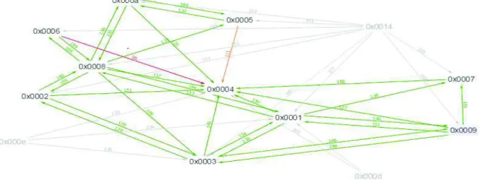
Our WSN consists of 11 fixed nodes initially deployed, 3 nomad nodes (the nodes 'D', 'E' and 'F'), and a mobile node (the node' C'). The positions of nomad nodes are determined by the proposed genetic algorithm. The mobile node is attached to a person moving within the 3D space of the building. Details and characteristics of the three indicated types of nodes are listed in table1 and table2. Figure 2 shows the RSSI links and the power of the received signal between the nodes of the network. The RSSI val-ues are indicated on the arcs (a value between 0 and 255 convertible in dBm). Blue arcs represent excellent links, green arcs rep-resent good connections, arcs in orange reprep-resent less good connections, and red arcs reprep-resent weak connections in terms of quality of the received signal.
Figure2. Network architecture.
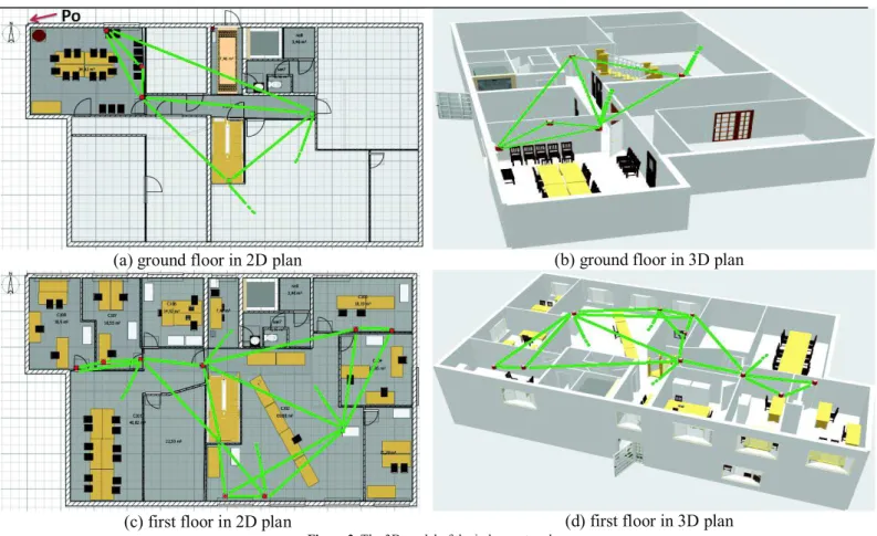
Figure 3 shows the deployment schema in the 2D plan and the 3D plane. The origin of our local coordinate system is set at the point P0(0,0,0) shown in Figure 3(a), the x-axis is the horizontal axis, the y-axis is the vertical axis, and the third axis will be for
(a) ground floor in 2D plan (b) ground floor in 3D plan
(c) first floor in 2D plan (d) first floor in 3D plan
Figure 3. The 3D model of the indoor network.
Table1 represents the technical and localization characteristics of the installed nodes (fixed and mobile nodes). Table 1. Technical and localization characteristics of the installed node.
No Hexadecimal
nomenclature
Decimal nomenclature
Type Position according to
the local coordinate
Means number of neighbors > threshold
Before the redeployment
X Y Z N1 0x0001 01 Teensy 3.0 mk20dx128 278 545 523 4, 3 N2 0x0002 02 Teensy 3.0 mk20dx128 1063 525 521 3,2 N3 0x0003 03 Teensy 3.0 mk20dx128 683 498 526 4,1 N4 0x0004 14 Teensy 3.1 mk20dx256 663 414 206 2,8 N5 0x0005 05 Teensy 3.0 mk20dx128 2093 305 519 3,5 N6 0x0006 06 Teensy 3.0 mk20dx128 1237 1256 443 3,7 N7 0x0007 15 Teensy 3.1 mk20dx256 450 00 290 2,9 N8 0x0008 1c* Teensy 3.1 mk20dx256 1114 1252 422 3,3 N9 0x0009 31* Teensy 3.1 mk20dx256 416 495 336 4,5 N10 0x000A 1F* Teensy 3.1 mk20dx256 1813 306 356 3,1 N11 0x000B 34* Teensy 3.1 mk20dx256 672 270 291 2,6 N15 0x000C C Teensy 3.1 mk20dx256 - - - -
Table2 represents the technical and localization characteristics of the nomad nodes added after the redeployment. Their positions are determined by our modified NSGAII algorithm.
Table 2. Locations of the nomad nodes according to our modified NSGAII algorithm.
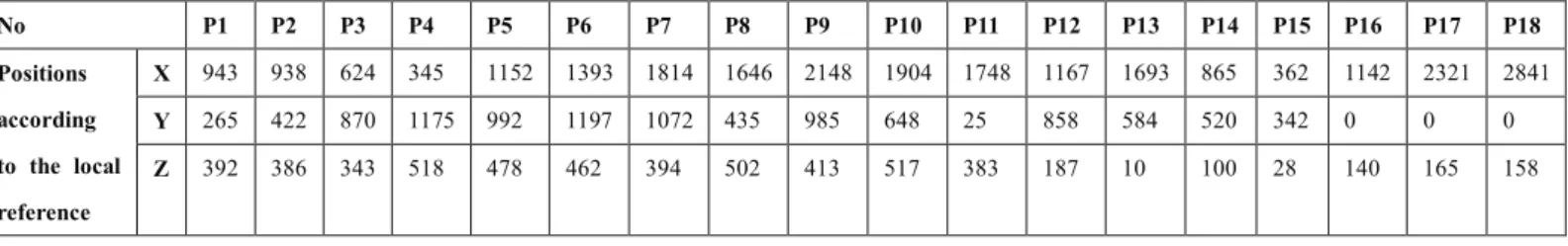
Table3 represents the location details of a set of selected positions on the 3D space to assess coverage and localization before and after the redeployment. These positions are chosen in different regions of the 3D space.
Table 3. Locations of selected positions taken by the mobile node 'C'.
No P1 P2 P3 P4 P5 P6 P7 P8 P9 P10 P11 P12 P13 P14 P15 P16 P17 P18 Positions according to the local reference X 943 938 624 345 1152 1393 1814 1646 2148 1904 1748 1167 1693 865 362 1142 2321 2841 Y 265 422 870 1175 992 1197 1072 435 985 648 25 858 584 520 342 0 0 0 Z 392 386 343 518 478 462 394 502 413 517 383 187 10 100 28 140 165 158 6.3 Objectives
Our goal is to add mobile nodes in the indicated locations while guaranteeing a set of network objectives and a set of ap-plication objectives. The applicative objectives are the metrics to measure: they are linked to existing sensors measuring physical parameters such as temperature brightness, or opening and closing doors. The network objectives mainly concern the measurement of the strength of the links between nodes over time: We evaluate the number of neighbors and the link quality (thus the radio coverage quality) by measuring the RSSI and the localization quality by measuring the FER. Ac-cording to OpenWino, the notion of a neighbor is defined as follows: a node 'b' is considered as a neighbor in the neighbor table of another node 'a' only if the power of the RSSI signal of 'b', received by 'a' is sufficient (greater than a predefined threshold taken to 100). Indeed, coverage is ensured if each node in the 3D space has at least one neighbor and if each tar-get in this space is monitored by at least one node. The localization is provided if all nodes have at least one neighbor. In our case, we use a hybrid 3D localization model (based on DVHop and RSSI) which requires that each node should have four neighbors. The measures are taken by day and night. The existence of a large number of people by day implies that the majority of doors are opened while the majority of doors are closed overnight, which influence the quality of the received signal. Indeed, anti-fire doors prevent the transmission of the signal and affect its quality.
No Hexadecimal
nomenclature
Decimal nomenclature
Type Position according to the local reference
X Y Z
N12 0x000D 58 Teensy 3.1 mk20dx256 1163 1004 192 N13 0x000E 59 Teensy 3.1 mk20dx256 1796 0830 501 N14 0x000F 60 Teensy 3.1 mk20dx256 1682 474 146
6.4 Evaluation of the Localization (Measurements and Interpretations)
To measure the localization, we use the RSSI metric since the used location model is based on RSSI and DVHop hybrid-ization (see Section IV). Therefore, more the RSSI is greater, more the localhybrid-ization is improved. A neighbor can enter in the neighbor table of a node only if the value of the RSSI of the detected node is greater than a predefined threshold. This threshold is configurable via the command "phy rssith set" [20]. The theoretical value of this threshold is fixed to 100. Based on our numerical results, we analyze the effect of the value of the RSSI threshold and its relationship with the FER. The value of the RSSI may change each period of time. This interval may be less than one second. Given this instability, we take for each pair of nodes (node i - node C); i ∈ [1,14]; an average value extracted from four values taken with an interval of 20 seconds between them.
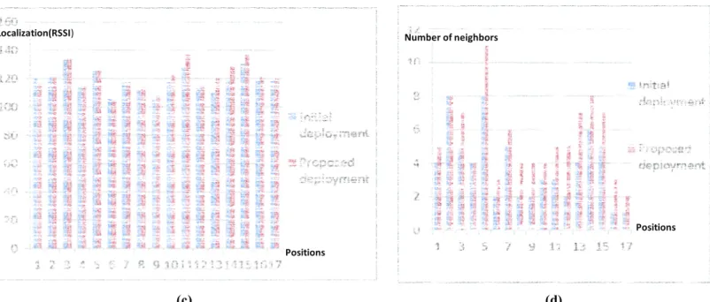
Figure 4(a) shows the variation of the localization (RSSI), before and after deployment, by day, for different positions. Figure 4(b) illustrates the variation of the number of neighbors before and after deployment, by day, for different positions. Figure 4(c) shows the change of location (RSSI), before and after deployment, overnight, for different positions. Figure 4(d) demonstrates the variation in the number of neighbors before and after deployment, overnight, for different positions.
0 20 40 60 80 100 120 140 160 180 1 2 3 4 5 6 7 8 9 10 11 12 13 14 15 16 17 Initial deployment Proposed deployment Positions (a) (b) Positions Number of neighbors Localization(RSSI)
(c) (d)
Figure 4. Variations on the localization (RSSI), before and after deployment, by day and night, for different positions.
Although the average number of neighbors (detected by the mobile node ‘C’) is higher at night, the average of the RSSI is higher by day (and then the localization is better by day). This is explained by the fact that the closed doors overnight prevent a good signal transmission. We summarize the variation rate and the localization improvements, after the deploy-ment phase as follows: By day, the localization rate is improved by +6.07% and the average number of neighbors (detecting 'C' and detected by 'C') is improved by 1.03. Overnight, the localization rate is improved by +5.96% and the average num-ber of neighbors (detecting 'C' and detected by 'C') is improved by 0.94.
6.5 Evaluation of the Coverage (Measurements and Interpretations)
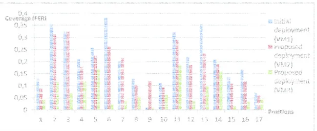
To measure the coverage, we use the frame error rate (FER) as a metric to evaluate the quality of links between nodes. Therefore, less the FER is higher, more the coverage is better. Although the values of the FER vary less than those of the RSSI, we take for each pair of nodes (node i - node C); i ∈ [1, 14]; an average value extracted from four values taken with an interval of 10 seconds between them. Figure 5 illustrates the variation of the coverage (FER), by day, for different posi-tions between the initial deployment (VM1), the proposed deployment with neighbors selected according to the maximum RSSI (VM2) and the proposed deployment with neighbors selected according to the minimum FER (VM3). Figure 6 illus-trates the variation of the coverage (FER), overnight, for different positions between the initial deployment (VM1), the proposed deployment with neighbors selected according to the maximum RSSI (VM2) and the proposed deployment with neighbors selected according to the minimum FER (VM3).
Positions Localization(RSSI)
Positions Number of neighbors
Figure 5. Variations of the coverage (FER), before and after deployment, by day, in different positions.
Figure 6. Variations of the coverage (FER), before and after deployment, overnight, in different positions.
Comparing the FER and the RSSI rates between day and night, we note that the FER rate is higher by day although the RSSI rate is higher: this indicates that the neighbors chosen according to the highest RSSI rates are not good neighbors. To prove this assumption, we compare the error rate after the deployment with neighbors selected according to the maximum RSSI and the error rate after the deployment with neighbors selected according to the minimum rate of FER: the compari-son (see VM2 and VM3 in Figure 5 and Figure 6) clearly indicates that the introduction of neighbors according to the highest RSSI does not always give the lowest error rate. By comparing the error rate before and after deployment, we con-clude that our approach has allowed the minimization of error rates and subsequently maximizing coverage.
We summarize the rate changes and the improvement of coverage and localization after the deployment phase as follows: -By day: coverage is improved by + 2.81% (a lower error rate) between the initial deployment and the deployment
posed by our approach. Coverage is improved by + 10.71% (a lower error rate) between the deployment proposed by our approach using a neighbor table based on the highest RSSI and deployment proposed by our approach with a neighbor table based on the smaller FER.
-Overnight: coverage is improved by + 3.87% (a lower error rate) between the initial deployment and the deployment proposed by our approach. Coverage is improved by + 3.28% (a lower error rate) between the deployment proposed by our approach using a neighbor table based on the highest RSSI and deployment proposed by our approach with a neighbor table based on the smaller FER.
7. Discussion
After the analysis of the experiment, different findings may be considered:
- In some cases, lower average of RSSI is recorded after the deployment. Despite this decrease indicating that the RSSI of the new nodes are worse than the RSSI of the installed nodes, localization rate, coverage rate and the number of neigh-bors are improved. Considering the goals set by our approach, this is understandable, since adding a node in a location x1 so that it is close to several nodes with a lower value of RSSI will be better than adding it in a location x2 with smaller number of neighbors and a higher RSSI value.
- It is noted that the node’s range is not spherical: according to measures, some nodes are detected by nodes that are fur-ther away than ofur-ther nodes which are not detecting them. For example, the node ‘N4’ is the only one detecting the node ‘C’ which is in the location P1 despite that there are other nodes which are less distant from the P1 location. Simulations should consider this assumption.
- After the capture of the values on the same position over several periods, we note that after a certain moment of initial-izing the links between nodes, the FER decreases (less error rate) and the RSSI increases (stronger signal).
- Also, from numerical results, we deducted the nature of the relationship between the RSSI and the FER: The theoretical RSSI threshold is fixed to 100 to ensure a good quality of links. Yet, sometimes a neighbor is introduced in the neighbor table based on a high RSSI rate but after a period of time, we find that the percentage of the lost frames is very high. Therefore, increasing the RSSI value may not decrease the FER value. Therefore, FER indicates the quality of links better than the RSSI.
8. Conclusion
This paper aims at providing a deployment scheme in 3D wireless sensor network while optimizing coverage and local-ization. The following objectives are considered: maximizing the coverage area and maximizing the precision localization in terms of the detection signal based on a DVHop algorithm which is corrected by the RSSI. We provide a genetic algorithm based approach that shows a significant performance improvement in quality of coverage and localization. We test our contributions in reality on a set of testbeds using the OpenWiNo emulator, by deploying nodes on the IUT of blagnac in Toulouse. We are interested in several directions in the future. We can further enhancing the proposed strategy to ensure the dynamic redeployment of nodes while considering different other objectives, such as the lifetime and the network connec-tivity. Moreover, as a prospect, we aim to intensify the deployed network by adding new nodes in order to better satisfy the localization constraint imposing four neighbours for each target. The experiment will be redone to study the influence of the network density on the results.
REFERENCES
[1] Maulin, P., Chandrasekaran, R. and Venkatesan, S., “Energy Efficient Sensor, Relay and Base Station Placements for Coverage, Connectivity and Routing,” IEEE International Performance, Computing and Communications Conference, pp. 581-586, 2005. [2] X. Cheng, DZ Du, L. Wang, and B. Xu, “Relay sensor placement in wireless sensor networks,” ACM/Springer Journal of Wireless
Networks, 14: pp. 347-355, 242, 2008.
[3] H. Qi, S. S. Iyengar, and K. Chakrabarty, “Multi-resolution data integration using mobile agents in distributed sensor networks”, IEEE Transactions on System, Man and Cybernetics (Part C), vol. 31, pp. 383-391, August 2001.
[4] S. S. Iyengar, L. Prasad and H. Min, “Adances in Distributed Sensor Technology,” Prentice Hall, Englewood Cliffs, NJ, 1995. [5] R. R. Brooks and S. S. Iyengar, Multi-Sensor Fusion: Fundamentals and Applications with Software, Prentice Hall, Upper Saddle
River, NJ, 1997.
[6] Mnasri S., Nasri N., Val T., “An Overview of the deployment paradigms in the Wireless Sensor Networks,” International Confer-ence on Performance Evaluation and Modeling in Wired and Wireless Networks (PEMWN 2014), Tunisia – 04-07th November 2014.
[7] Mnasri S., Thaljaoui A., Nasri N., Val T, “A genetic algorithm-based approach to optimize the coverage and the localization in the wireless audiosensors networks,” IEEE International Symposium on Networks, Computers and Communications (ISNCC 2015), Hammamet, Tunisie, IEEExplore digital library, p. 1-6, Mai 2015 (to appear).
[8] A. Howard, M. J. Matari´c and G. S. Sukhatme, “Mobile Sensor Network Deployment Using Potential Field: a distributed scalable solution to the area coverage problem”, in Proc. International Conference on Distributed Autonomous Robotic Systems”, June 2002.
[9] A. Konstantinidis, K. Yang, Q. Zhang, and D. Zeinalipour-Yazti, “A multi-objective evolutionary algorithm for the deployment and power assignment problem in wireless sensor networks,” Computer Networks 54(6): 960-976, 2010.
[10] O. Banimelhem, M. Mowafi, and W. Aljoby, “Genetic Algorithm Based Node Deployment in Hybrid Wireless Sensor Networks,” Communications and Network, 5, 273-279. Published Online November 2013 (http://www.scirp.org/journal/cn) http://dx.doi.org/10.4236/cn.2013.54034
[11] K. J.Aval and S. Abd Razak, “A Review on the Implementation of Multiobjective Algorithms in Wireless Sensor Network,” World Applied Sciences Journal 19 (6): pp. 772-779, ISSN 1818-4952, 2012; DOI: 10.5829/idosi.wasj.2012.19.06.1398
[12] Y. Qu, “thesis: Wireless Sensor Network Deployment,” Florida International University, Miami, Florida, USA, defense: March, 26th 2013.
[13] N. Bulusu, J. Heidemann and D. Estrin, “Adaptive beacon placement”, Proc. International Conference on Distributed Computing Systems, pp. 489-498, 2001.
[14] S. Meguerdichian, S. Slijepcevic, V. Karayan and M. Potkonjak, “Coverage problems in wireless ad-hoc sensor networks”, Proc. IEEE Infocom, vol. 3, pp. 1380-1387, 2001.
[15] L. Zhang, X. Zhou, and Q. Cheng, “Landscape-3D: a robust localization scheme for sensor networks over complex 3D terrains,” in Proceedings of the 31st Annual IEEE Conference on Local Computer Networks (LCN ’06), pp. 239–246, November 2006. [16] Baohui Zhang, Guojun Dai, Jin Fan, and Tom H. Luan, “A Hybrid Localization Approach in 3D Wireless Sensor Network,”
Inter-national Journal of Distributed Sensor Networks, Article ID 692345, in press.
[17] T.He, C.Huang, B.M. Blum, J. A. Stankovic, and T. Abdelzaher, “Rangefree localization schemes for large scale sensor networks,” in Proceedings of the 9th Annual International Conference on Mobile Computing and Networking (MobiCom ’03), pp. 81–95, 2003.
[18] N. Bulusu, J. Heidemann, and D. Estrin, “GPS-less low-cost outdoor localization for very small devices,” IEEE Personal Commu-nications, vol. 7, no. 5, pp. 28–34, 2000.
[19] G. Tan, H. Jiang, S. Zhang, and A.-M. Kermarrec, “Connectivity- based and anchor-free localization in large-scale 2D/3D sensor networks,” in Proceedings of the 11th ACM International Symposium on Mobile Ad Hoc Networking and Computing (MobiHoc ’10), pp. 191–200, September 2010.
[20] Adrien VAN DEN BOSSCHE, Thierry VAL, “OpenWiNo : une plateforme de prototypage rapide pour l'ingénierie des protocoles dans les Réseaux de Capteurs Sans Fil et l'Internet des Objets “, Days : « L'Internet des Objets : du concept à la pratique », INSA Toulouse, France, May 2014.