Generalized Geometry Projection: A Unified Approach for Geometric Feature Based Topology Optimization

an author's https://oatao.univ-toulouse.fr/24589

https://doi.org/10.1007/s11831-019-09362-8

Coniglio, Simone and Morlier, Joseph and Gogu, Christian and Amargier, Rémi Generalized Geometry Projection: A Unified Approach for Geometric Feature Based Topology Optimization. (2019) Archives of Computational Methods in Engineering. 1-38. ISSN 1134-3060

(will be inserted by the editor)

Generalized Geometry Projection:

A Unified Approach for Geometric Feature Based Topology Optimization

Simone Coniglio · Joseph Morlier · Christian Gogu · R´emi Amargier

Received: date / Accepted: date

Abstract Structural topology optimization has seen many methodological advances in the past few decades. In this work we focus on continuum-based structural topology optimization and more specifically on geomet-ric feature based approaches, also known as explicit topology optimization, in which a design is described as the assembly of simple geometric components that can change position, size and orientation in the con-sidered design space. We first review various recent de-velopments in explicit topology optimization. We then describe in details three of the reviewed frameworks, which are the Geometry Projection method, the Moving Morphable Components with Esartz material method

S.Coniglio

Airbus Operations S.A.S. 316 route de Bayonne 31060 Toulouse Cedex 09 France Tel.: +33 (0)561937259 E-mail: simone.coniglio@airbus.com J. Morlier

Institut Clment Ader (ICA), CNRS, ISAE-SUPAERO, UPS, INSA, Mines-Albi,

3 rue Caroline Aigle, 31400 Toulouse, France

E-mail: j.morlier@isae-supaero.fr C. Gogu

Institut Clment Ader (ICA), CNRS, ISAE-SUPAERO, UPS, INSA, Mines-Albi,

3 rue Caroline Aigle, 31400 Toulouse, France R. Amargier

Airbus Operations S.A.S. 316 route de Bayonne 31060 Toulouse Cedex 09 France

and Moving Node Approach. Our main contribution then resides in the proposal of a theoretical framework, called Generalized Geometry Projection, aimed at uni-fying into a single formulation these three existing ap-proaches. While analyzing the features of the proposed framework we also provide a review of smooth approx-imations of the maximum operator for the assembly of geometric features. In this context we propose a satu-ration strategy in order to solve common difficulties en-countered by all reviewed approaches. We also explore the limits of our proposed strategy in terms of both simulation accuracy and optimization performance on some numerical benchmark examples. This leads us to recommendations for our proposed approach in order to attenuate common discretization induced e↵ects that can alter optimization convergence.

Keywords Topology Optimization _{· Geometry}

Projection· Moving Morphable Components · Moving Node Approach_{· Smooth Geometry assembly}

1 Introduction

The manufacturing industry is faced with multiple chal-lenges in both cost reduction and product performance improvement in order to stay competitive in the market. In this context, structural optimization is a key feature for improving existing products and finding disruptive concepts. In particular, topology optimization appears quite promising in this context, as it deals with the de-termination of the optimal structural layout, given var-ious performance objectives and constraints. For this reason it can be used to inspire non-conventional solu-tions or derive design principles for similar problems. Since the pioneering work of [5], topology optimization

has received considerable research attention. Numer-ous topology optimization approaches such as SIMP (Solid Isotropic Material with Penalization) approach [4, 76], level set approach [1, 50], and evolutionary ap-proach [54,56] have been successfully proposed and im-plemented. Direct density based approaches [4, 6, 76], which are currently among the most popular ones, can reach organic or free form designs, defining the local presence or absence of material. In Zhu et al. [81], the interested reader can find a review of this family of approaches in the Aerospace design applications. The exploration power of these approaches, their freedom and their ease in handling large changes in the design configuration without re-meshing come however at the cost of some drawbacks as well:

– The number of design variables and of degrees of freedoms in the finite element model grows quite fast in 3D problems and their resolution becomes quickly prohibitive especially if considering optimization for-mulation that do not only include compliance and volume fraction.

– The typical ”bionic” designs obtained with direct density based methods, even if highly e↵ective, may not be easily compatible with manufacturing require-ments (e.g. casting, rolling, overhang angle constraints, etc). Indeed as analyzed in the recent survey by Liu and Ma [30], and more recently of Liu et al. [29] the implementation of manufacturing considerations in topology optimization is still a challenging, highly active area of research.

– Intermediate densities often subsist in the final de-sign in direct density based approaches due to com-putational cost constraints, preventing the full con-vergence towards black and white designs. The gray elements would then have to be threshold to black and white solutions, which can lead to a loss in per-formance compared to the optimum.

– The density formulation of the topology optimiza-tion problem is ill posed and need to be transformed into a well posed one through restriction to feasible set of solutions [7]. Some approaches like mesh in-dependent filter techniques [41], depending on the filter size, can be computationally expensive. An alternative family of approaches seeks to both use geometric primitives (i.e. geometric components) to define the optimal solution and inherit a fixed mesh as typical in direct density based topology optimization. In the literature one can find two major groups of ap-proaches incorporating geometric features in topology optimization:

– A first group combines the free-form topology opti-mization with embedded components or holes shaped

as geometric primitives. (c.f. Chen et al. [9];Qian and Ananthasuresh [38]; Xia et al. [55]; Zhang et al. [69, 73]; Zhou and Wang [77]; Zhu et al. [80]) – A second group, to which this work belongs,

repre-sent the solution only by means of geometric primi-tives. Norato [36] provides an extensive description of works dealing with these approaches. The pre-cursor of these methods is the bubble method (Es-chenauer et al. [14]), one of the first form of topology optimization. Still this approach require re-meshing during the optimization process which a↵ects its computational burden. Another work that can be consider as belonging to this category is the Feature-based topology optimization [11], where the struc-ture is obtained as the results of Boolean operations over simple geometric feature structures, in this case holes. The same author proposes in [10] an implicit control of the solution quality using a quadratic term of the energy in the formulation of the op-timization problem. In the work of Seo et al. [40], the solution is described using trimmed spline sur-faces and the isogeometric analysis. In the Adaptive Mask Overlay Topology Synthesis Method, Saxena et al. [39] circular, rectangular or elliptical holes are considered in the solution and the structural analysis is performed on the remaining solid struc-ture using hexagonal elements. A similar approach is applied by Wang et al. [49]: a fixed mesh is em-ployed this time and a regularized Heaviside func-tion is used to evaluate the mechanical properties on a fixed finite element mesh. Liu et al [31] proposed to use Compactly supported Radial basis functions to interpolate simple geometric features in a level set topology optimization framework. The performance of the resulting structure was then computed thanks to the extended finite element method (XFEM). In the ISOCOMP approach of Lin et al. [26], the simul-taneous optimization of both the location of holes and the layout of material is studied with the use of both isogeometric analysis and the Hierarchical Par-tition of Unity Field Compositions (HPFC) theory, which is employed for both geometry and solution field approximations.

In this second family of methods, four approaches represent a solution as the union of geometric entities that can move, stretch and analytically modify their shapes: the moving morphable components (MMC) method (Guo et al. [16, 17], Zhang et al. [64, 71]) ; the geome-try projection (GP) method (Bell et al. [3], Norato et al. [35], Zhang et al. [62]); the Method of Moving Mor-phable Bars (MMB) Hoang et al. [19] and the Moving Node Approach (MNA), introduced in the Master

the-sis of Overvelde [37]. We refer to these approaches as explicit topology optimization approaches, highlighting the fact that the material description is explicitly de-scribed, instead of implicitly as it is the case for di-rect density based approaches, where the layout is de-scribe by a mapping of presence and absence of ma-terial. In [17], an explicit level set function is used to determine the geometry of moving morphable compo-nents with uniform thickness. The XFEM approach was employed as an alternative for the displacement com-putation [24, 48, 53]. The same framework is also pre-sented in Zhang et al. [72] where MMC is identified as a way of extending techniques commonly employed in shape optimization, with the freedom inherited from topology optimization. Moving components with vari-able thickness are used in [71], and the esartz material model is employed to enhance computational efficiency. In the work of Zhang et al. [65] length scale control is achieved by directly controlling the component’s mini-mal thickness. In Deng et al. [12] the MMC approach is successfully implemented to solve various types of prob-lems, like the design of compliant mechanisms and of low-frequency resonating micro devices. In the work of Zhang et al. [64], the MMC framework is extended to 3D structures. The complexity of the solution is con-trolled in [74] by controlling the maximum number of components in the final solutions.

The Moving Morphable Voids approach [63] makes use of b-splined shaped holes, explicitly piloted in the topology optimization. The proposed framework, not only reduce the optimization burden due to variables reduction, but also impacts the cost of the evaluation of the displacement field, eliminating the element com-pletely contained in the void region from the analysis. The same framework is applied to tackle stress based topology optimization in [66]. In Zhang et al. [70] the control of the solution is achieved by varying explic-itly the boundaries of Components or voids using B-spline curves. In Takalloozadeh et al. [47] the topolog-ical derivative is implemented in the MMC approach. In the work of [18] the ability of MMC to determined self supported structures is studied and in Liu et al. [27] the MMCs/MMVs framework is employed to determine graded lattice structures achievable with additive layer manufacturing technologies. In Hou et al. [20] the MMC framework is proposed based on Isogeoemtric Analy-sis (IGA) instead of finite element analyAnaly-sis (FEA). In Zhang et al. [68], the MMC approach is employed to de-sign multi-material structures and in Zhang et al. [67] it is employed to find the best layout of sti↵ening ribs in-cluding buckling constraints. Geometric non-linearities are considered in Zhu et al. [79] for MMC and in Xue et al. [57] for MMV. In Lei et al. [25] machine learning

techniques like: support vector regression (SVR) [42] and the K-nearest-neighbors (KNN) [2], were adopted in order to speed up the resolution of the optimization problem, under MMC framework. In Liu et al. [28] an efficient strategy is proposed to decouple the finite ele-ment mesh discretization from the discretization em-ployed to assemble the sti↵ness matrix on the basis of the geometric configuration. In Sun et al. [43] the topology optimization of a 3D multi-body systems con-sidering large deformations and large overall motion is achieved using MMC.

With the Method of Moving Morphable Bars (MMB) Hoang et al. [19] introduce round ended bars in the topology optimization framework that can overlap and change both shape and position. As main features of this work one can identify the control of both mini-mal and maximini-mal thickness of the components, the use of sigmoid Heaviside function to project the compo-nents on the fixed finite element mesh, the use of SIMP material model to penalize intermediate density and the boolean union of components realized making the product of Heaviside functions. MMB was also stud-ied in wang et al. [51] for the layout of planar multi-component systems.

The Geometry Projection (GP) approach was initially introduced by Norato et al. [34], for the shape optimiza-tion of holes over a fixed finite element mesh. This basic idea was developed further by Bell et al. [3] to make the topology optimization of structures composed by rect-angular components in 2D, by Norato et al. [33] using 2D round ended bar components that can both overlap and merge. The same author proposed to use this ap-proach to find the best distribution of short fiber rein-forcement in [35]. In Zhang et al. [62] Geometry projec-tion approach was implemented for 3D solid structures composed of rectangular plates. In Zhang et al. [58] stress based topology optimization is conducted on 2D topology optimization problems, using GP. The design of unit cells for lattice materials in 3D is considered in Watts et al. [52]. In Zhang et al. [59] curved plates are considered as building blocks of 3D topology optimiza-tion problems using GP. In Zhang et al. [60] Geometry Projection was employed to design the rib reinforce-ment of plates in 3D. In the work of Norato [36] su-pershapes geometric features are employed as building blocks in a 2D topology optimization framework based on geometry projection. In Kazemi et al. [21], the Ge-ometry Projection was applied to multi-material design of 2D and 3D structures. In Zhang et al. [61] a tunnel-ing strategy is proposed to alleviate the initial point dependency in Geometry projection.

It is clear that the domain of explicit topology op-timization is currently a very active area of research.

We chose to focus in this paper on the following three frameworks, which follow di↵erent approaches for achiev-ing explicit topology optimization: the Movachiev-ing Mor-phable Components (MMC) with Esartz material ap-proach, the Geometry Projection (GP) approach and Moving Node Approach (MNA). The main goal of this paper is to propose a generalized theory, that we call Generalized Geometry Projection (GGP), of which all three approaches can be seen as particular cases. A fur-ther contribution resides in the proposal of a specific saturation strategy, that can be adopted to overcome the difficulties that can be encountered in the assembly of geometric features, required in all considered explicit topology optimization approaches. Finally, a root cause of optimization convergence difficulties is extensively analyzed and possible solutions to circumvent this is-sue are discussed.

The remainder of this paper is structured as follows: Section 2 first introduces the geometric description of the components employed in this work and the com-mon steps undertaken by all three reviewed topology optimization approaches. We then review Moving Mor-phable Components (MMC) with Esartz material, Ge-ometry Projection (GP) and Moving Node Approach (MNA) in subsections 2.1,2.2 and 2.3 respectively. The proposed Generalized Geometry Projection that uni-fies all three approaches is presented in subsection 2.4. The techniques employed to obtain the geometric as-sembly are reviewed in subsection 2.5 and the sensitiv-ity chain is detailed in subsection 2.6 with the aim of providing practical implementation recommendations. A benchmark problem is then considered in section 3: the parametric study of a cantilever beam is conducted in subsection 3.1 and the topology optimization of a short cantilever beam is solved in subsection 3.2. Dis-cussion of the results and final recommendations are provided in section 4. Finally, conclusions and future work perspectives are outlined in section 5.

2 Methods

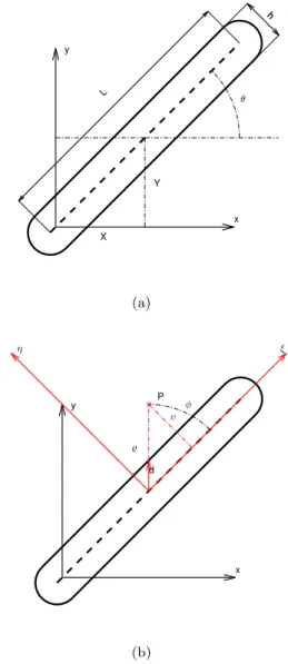
In this section we first describe three of the existing 2D explicit topology optimization approaches: Moving Morphable Components (MMC) with Esartz material model; Geometry Projection (GP); Moving Node Ap-proach (MNA). Then we describe the proposed method: Generalized Geometry Projection (GGP), aimed at uni-fying into a single formulation these three existing ap-proaches. To simplify the equations we will consider the same geometric components proposed in Norato et al. [35] for all reviewed approaches c.f. figure 1a. This component is defined by five geometric parame-ters defining the position of the center of the

compo-nent _{{X, Y }, the components dimensions {L, h} and} the component’s orientation {✓} . The final topology will then be described as a superposition of multiple such basic components. In this section we will refer to ! as the area occupied by a geometric component and to @! as its boundary. If more than one component is used to describe the area occupied by material, then we will refer to !i and to @!i as the ithcomponent’s area and boundary respectively. We will refer to ! and to @! as area and boundary of the union of all components i ( ! =[n

i=1!i). In order to define explicitly the

con-L hh Y X x y (a) d x y P (b)

Fig. 1: Geometric primitive (i.e. basic geometric compo-nent) used for all the reviewed methods. (a) The explicit geometric parameters associated to the component are {X, Y, L, h, ✓} . (b) Plot defining the local polar coordi-nates_{{%, }}T_{, the distance from the component} bound-ary d, and the distance from the component middle axis

tour of this component, we introduce polar coordinates {%, }T _{as defined in figure 1b. We refer to d as the} ra-dial distance of the component’s center_{{X, Y }}T _from the component boundary @! that can be computed as a function of the angle and of the component sizes L and h as: d( , L, h) = 8 < : q h2 4 L2_sin 2 4 + L 2| cos | if cos 2 L2 L2_+h2, h 2| sin | otherwise. (1) This piece-wise definition is at least of class C1_(R). Given a point _{Xg} ⌘ {x, y}T 2 R2, its polar coor-dinates can be defined as:

%(x, y, X, Y ) =p(x X)2_{+ (y Y )}2 ₍₂₎ (x, y, X, Y, ✓) = ( arctan⇣_{x X}y Y⌘ ✓ if x_{6= X,} ⇡ 2sign(y Y ) ✓ if x = X. (3) A consequence of the above definitions we have:

{Xg} 2 ! [ @! , d( , L, h) %(x, y, X, Y ) (4) Another way of describing the same component is by the use of the signed distance as described in Norato et al. [35]:

&( , h) := h

2 (5)

where is the distance from a point{Xg} 2 R2 to the component medial axis, which can be further expressed as a function of _{Xg}’s polar coordinates:

(%, , L, h) = 8 < : q %2₊L2 4 %L| cos | if % 2_cos 2 L2 4, %_{| sin |} otherwise (6) Accordingly, {Xg} 2 ! [ @! , &( , h)  0 (7)

The structural model used during the topology opti-mization will then be described by n components, each involving following six1 _{design variables}

{xi} = {Xi, Yi, Li, hi, ✓i, mi}T . For the whole structure involving n components the structural performance will thus depend on 6n design variables denoted as vector {x}: {x} = 8 > > > < > > > : {x1} {x2} .. . {xn} 9 > > > = > > > ; (8) 1 _{additional variable m}

iis introduced in the geometry

pro-jection approach to make a component vanish in the same way as it is done in density based approaches.

Each of the reviewed methods has its own way of up-dating the structural model that is used to evaluate the performance of a given design. A common feature is the fact that a linear elastic-static finite element model is employed. Here a structured uniform mesh based on dx_{⇥ dx solid elements in plane stress is adopted, where} dx is the element x and y size. The Poisson ratio ⌫ and the thickness t in the out of plane direction consid-ered to be a constant over all the design domain D. The Young’s modulus E depends on the fact that the consid-ered point belongs or not to !. A common assumption is that the Young’s modulus is piece-wise uniform over each element. For this reason, the elementary sti↵ness matrices [Kel_{] are all of the same form i.e:}

[Kel] = Eel[K0] el = 1, 2, ..., N (9)

where Eel _{is the Young’s modulus of the el}th _element, [K0] is the 8⇥ 8 sti↵ness matrix of a dx ⇥ dx 2D solid element in plane stress condition with thickness t = 1 and N is the total number of elements in the structural model. Using classic finite element theory, one can as-sembly the global sti↵ness matrix [K]:

[K] = N M el=1

[Kel] (10)

This is used to write the static balance equation in terms of the free degrees of freedoms{U} as:

[K]_{{U} = {F }} (11)

where_{{F } is the external loads vector. If the boundary} conditions are at least isostatic and Eel _E

min > 0, then the system of equation [K] is non-singular and the system of equation (11) can be solved to find the displacement vector_{U}.

{U} = [K] 1

{F } (12)

In many topology optimization formulations the mass of the structure is also of interest, which is usually con-sidered in terms of the volume fraction V associated to a given structural design layout (since V is proportional to the mass of a solution for a homogeneous material). To compute this volume fraction V the local density ⇢el are determined based on the design vector {x} as will be presented in details in the next subsections for each approach.

As an example of a topology optimization formula-tion within this framework we provide in eq. (13) the classical formulation consisting in minimizing the com-pliance of the structure (i.e. maximizing its sti↵ness)

subjected to a volume fraction constraint and design space constraints: 8 > > > > < > > > > : min_{x}C =_{U}T {F } s.t. V = PN el=1⇢ el N  V0 {lb}  {x}  {ub} (13)

Where {lb} and {ub} are respectively the vectors of lower bound and upper bound for the design variables and V0is the maximum allowed volume fraction in the final solution.

2.1 Moving Morphable Components (MMC) with Esartz material model

In this section we review the moving morphable compo-nents (MMC) method (Guo et al. [16,17]). MMC inher-its from the level set method [1] a Topology Description Function (TDF), that is positive inside the area occu-pied by the union of all components !, equal to zero on the boundary @! of the component and negative outside the component. The TDF values are then used either to apply the XFEM [53] on the boundaries of the components either to compute the element sti↵ness matrix using ersatz material model [71]. In this paper will focus on the application of the latter. The reader must note that we made some minor modifications to the original formulation, in order to include the round ended bar components (cf. Fig. 1a) with uniform thick-ness. The structural topology description is obtained using a topology description function (TDF), denoted

, that satisfies following relations: 8 > < > : > 0 if {Xg} 2 !, = 0 if _{Xg} 2 @!, < 0 if {Xg} 2 D\!. (14)

where D represents the total area of the design domain (full and voids). When more than one component is considered, the TDF of each component, denoted as

i= i({Xg}), is defined 8i = 1, .., n such that: 8 > < > : i> 0 if {Xg} 2 !i, i= 0 if {Xg} 2 @!i, i< 0 if {Xg} 2 D\!i. (15) Since ! =_[n

i=1!i one can verify that = maxi i sat-isfies the conditions (14). Given a component described by the geometric variables _{Xi, Yi, Li, hi, ✓i} we have several choice for defining the TDF i({Xg}). Here we

consider the following relationship, which has the ad-vantage of allowing simple derivations:

i= 1 ✓₄ 2 i h2 i ◆↵ with ↵ 1 (16)

Figure 2 illustrates the contour plot of the TDF i con-tour of the generic component of figure 1a.

-70 -70 -60 -60 -50 -50 -40 -40 -30 -30 -20 -20 -20 -20 -10 -10 -10 -10 -10 0 0 0 0 0 x y

Fig. 2: (_{Xg}) contour plot of the generic component of figure 1a. We considered ↵ = 1, X = 1, Y = 1, L = 3, h = 0.5, ✓ = ⇡

4. The domain D of the plot is [ 1, 2.5]_{⇥ [ 1, 2.5]}

Fig. 3: H✏( ({Xg})) filled contour plot of the compo-nent in figure 1a. We considered ↵ = 1, X = 1, Y =

1, L = 3, h = 0.5, ✓ = ⇡

4, = 0.01, ✏ = 0.6. The domain D of the plot is [ 1, 2.5]⇥ [ 1, 2.5]

The presence or absence of material in the design under consideration can be obtained by the Heaviside function H(x), applied to the topology description func-tion of the union of all the components . In order to

have a regular behavior of the optimization problem re-sponses, the Heaviside function H(x) is replaced by a regularized version H✏(x): H✏(x) = 8 > > < > > : 1, if x > ✏, 3(1 ) 4 ⇣ x ✏ x3 3✏3 ⌘ +1+₂ if ✏_{ x  ✏,} otherwise. (17) Where 0 < ✏ < 1 is a parameter that controls the am-plitude of the transition between the minimum value of (0 < << 1) and 1. The same generic component is used in figure 3 to plot H✏( ({Xg})). One can observe that the smooth variation, from a value of 1 inside the component to a value of outside it, is localized in a small transition zone, denoted Dg, that can be deter-mined using equations (16)-(17):

DM M Cg = ⇢ {Xg} | h 2 (1 ✏) 1 2↵ _{ } h 2(1 + ✏) 1 2↵ (18) The width of this transition zone is denoted by wg:

wM M Cg =

h 2 h

(1 + ✏)2↵1 _{(1 ✏)}2↵1 i ₍₁₉₎

A peculiarity of MMC is that the width of the tran-sition zone is directly proportional to the the compo-nent’s thickness h. A direct consequence is that smaller components will have faster variation between full ma-terial and voids. The e↵ect of this behaviour on the ill conditioning of the optimization problem will be inves-tigated on numerical examples in the implementation section.

According to [15], the value of the Young’s modulus in the elth_{-element is considered to be:}

Eel=

E⇣P4_j=1(H✏( elj))q ⌘

4 (20)

Where el

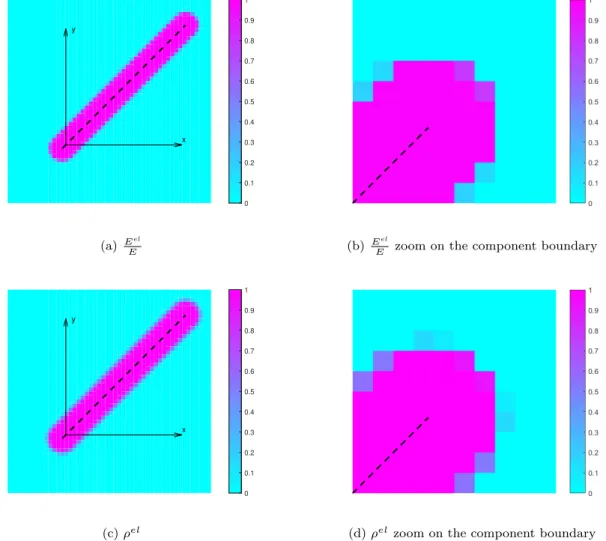
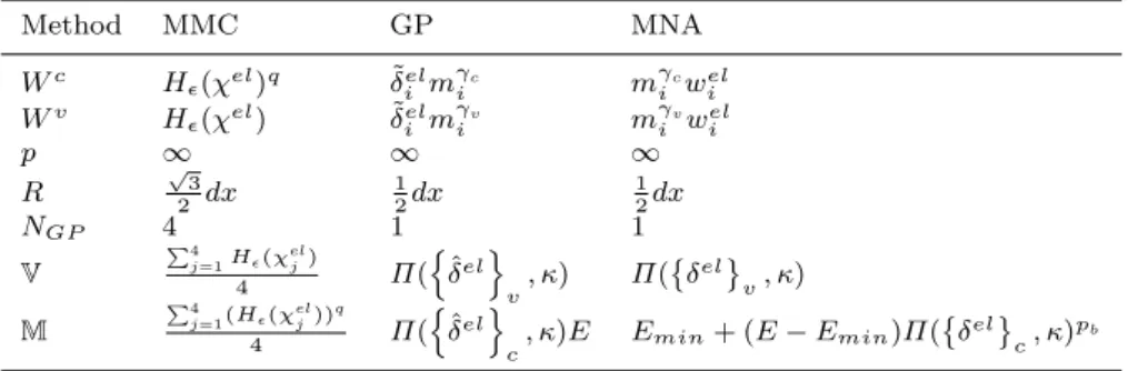
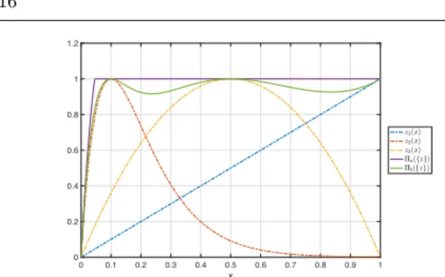
i ,i = 1, ..., 4 are the values of the TDF at the four nodes of the element el and q is a parameters that has the role of penalization, in order to render the varia-tion of Young’s modulus even faster at the boundary of the component. In figure 4a, the single component ex-ample of figure 1a has been used to plot the distribution of Young’s modulus according to equation (20) over a 50_{⇥50 finite element mesh. In order to obtain the local} density ⇢el_{, which was not explicitly considered in [71],} an equivalent expression that leads to the same value of volume fraction for the same configuration is proposed here:

⇢el= P4

j=1(H✏( elj))

4 (21)

In figure 4c the corresponding distribution of ⇢el_{is also} represented. Figures 4c and 4a look very similar except for the transition on element boundary that is faster for the Young’s modulus plot due to the e↵ect of the penalization parameter q.

2.2 Geometry Projection (GP)

In this section we review the approach proposed by No-rato et al. [35]. Geometric projection first computes the signed distance between each element central point and each component surface. The element local volume frac-tion is then computed by the mean of a spherical sam-pling window centred in the element centroid. Density and Young’s modulus in the element are computed as function of the volume fraction of the sampling window that is occupied by material. The density coming from each component is unified using the maximum function or its smooth approximation [23]. The solution is de-scribed by the union of geometric primitives such as the one in figure 1a. To update model densities the ge-ometry projection method is employed [34]. A circular sampling window Br

P of radius r is considered around the elth_{-element center X}el

g c.f. figure 5. The local volume fraction el _{is simply given by the fraction of} the window that is filled with material:

el i = |B r P \ !i| |Br P| (22) where _{| · | denotes the measure of the area. The} de-nominator can be computed analytically as the area of the circle|Br

P| = ⇡r2. The numerator of equation (22) on the other hand is more complex but can be approx-imately computed with the assumption that r is small enough. In this case the restriction of @! to the circle BrP can be considered as a straight line. As a conse-quence one can compute:

el i ⇡ 8 > < > : 0 if & > r, 1 ⇡r2 ⇥ r2_arccos & r & p r2 _&2⇤ _{if r &  r,} 1 otherwise. (23) Where the signed distance & (cf. eq. (5)) is computed in the elth_{element centroid X}el

g and with respect to the ith _{component. In order to avoid sti↵ness matrix} singularities, the local densities are modified as follows.

˜el

x y 0 0.1 0.2 0.3 0.4 0.5 0.6 0.7 0.8 0.9 1 (a) Eel E (b) Eel

E zoom on the component boundary.

x y 0 0.1 0.2 0.3 0.4 0.5 0.6 0.7 0.8 0.9 1

(c) ⇢el _{(d) ⇢}el _{zoom on the component boundary.}

Fig. 4: Distribution ofEel

E (a-b) and ⇢

el _{(c-d) for the generic component of figure 1a and for a 50}

⇥ 50 FE mesh over the domain of Xg. The same parameters of figure 3 are also considered here with q = 2.

where min is the minimum of local volume fraction to be considered in the analysis. Moreover:

ˆel

i (mi, ) = ˜ielmi (25)

Where mi is the ith component mass or out of plane thickness [35] and 1 penalizes the intermediate value of the component’s mass. The local densities are finally computed by taking the union of all the compo-nents using a smooth approximation of the maximum function:

⇢el( v, ) = ⇧({ˆel({m} , v)}, ) (26) where  is an aggregation constant and_{ˆel₍

{m} , v)} is the vector of local density stemming from each com-ponent. Here we do not specify the form of the smooth approximation of the maximum function ⇧, which will be investigated in details in the implementation section.

In order to determine the value of the Young’s modu-lus of an element, the following equation is used which involves a second penalty parameter c > v

Eel_{= ⇢}el₍

c, )E (27)

This penalization is very similar to the one adopted by the SIMP approach and is e↵ective in order to pro-gressively eliminate a component with an intermediate value of mithroughout the optimization iterations [35]. In figure 6, the generic component of figure 1a is consid-ered to show the distribution of both Young’s modulus and element densities over a 50_{⇥ 50 mesh. Note again} that the transition zone from full material to void is concentrated on the boundary of the component: DgGP = ⇢ {Xg} | h 2 r  h 2 + r (28)

Fig. 5: Basic component and notations associated to the Geometry Projection method [35]

x y 0 0.1 0.2 0.3 0.4 0.5 0.6 0.7 0.8 0.9 1 Fig. 6: Distribution of Eel

E for the generic component of figure 1a and for a 50⇥ 50 mesh over the domain of Xg. We considered X = 1, Y = 1, L = 3, h = 0.5, ✓ =

⇡

4, c = 3, r = 0.105, min= 10

6_{. Due to the choice of} m = 1 the same distribution is obtained for ⇢el_.

As a consequence this time the thickness of the transi-tion zone is:

wGPg = 2r (29)

This thickness does not depend on the component size h. In order to achieve regular density distributions, h will need to be greater or equal than 2r. To delete in-active components, variable m can still be used within the optimization algorithm.

2.3 Moving Node Approach (MNA)

Overvelde [37], proposed in his master’s thesis an al-ternative flow-inspired topology optimization approach, the Moving Node Approach (MNA). For this approach, the building blocks of a solution are defined as mass nodes. Each element’s center position is recomputed with respect to a local coordinate system in each com-ponent center . Then weighting functions are directly applied to the local variable to compute the compo-nent local density contribution. In order to compute the union between the components, this time, the den-sities are summed. Since the sum can be greater than one, to keep the resulting density bounded from 1 an adapted procedure was proposed in [37] called asymp-totic density. Another peculiarity of Overvelde work was the fact of using either Finte Element Analysis or meshless method (cf. [32]) for the displacement eval-uation. The idea was to reduce both design variable and degrees of freedom number, using the mass nodes for both the geometric description and the solution dis-placement. Unfortunately in [37] the gain in dofs num-ber was compensated by the sti↵ness matrix cost (both in memory and elapsed time) and by its ill conditioning where the mass nodes reached each other. The update of the finite element model is done by operating through weighting functions w that are driven by the geometry of each component. In this paper we considered a mod-ified weighting function with respect to [37] in order to consider round ended bar components. For the mass node of figure 1a one can write:

w( , h, ") = 8 > < > : 1 if _{ l,} a3 3+ a2 2+ a1 + a0 if l < < u, 0 otherwise. (30) Where l = h 2 " 2 (31) u = h 2 + " 2 (32) a3= 2 "3 (33) a2= 3h "3 (34) a1= 3 h2 _"2 "3 (35) a0= (h + ") 2_{(h 2")} 4"3 (36) (37) The local density can then be computed as:

el

Where we call el

i the distance from the elth element centroid Xel

g to the ithcomponent middle axis com-puted using equation (6). To make the union of all mass nodes a smooth approximation of the maximum func-tion is again typically employed:

⇢el= ⇧(_{{ }}el_v , ) (39)

Finally the Young’s modulus is updated using a power law:

Eel= Emin+ (E Emin)(⇧({ }elc , ))pb (40) Where pb 1 is used to penalize intermediate densities. In figures 7a,7c both Young’s modulus distribution and densities are considered for the same generic component and same mesh as for figures 4a,4c and 6. Note that in this case as well the gray region is localized in the transition zone defined this time by:

DM N Ag = ⇢ {Xg} | h " 2   h + " 2 (41)

The thickness of this transition zone is then defined as:

wM N Ag = " (42)

This thickness is, as for Geometry Projection, indepen-dent from the component thickness h. On the other hand one can observe in figure 7a, compared to Geom-etry Projection, the e↵ect of the penalty pb > 1 that reduces the value of the densities in the transition zone.

2.4 Generalized Geometry Projection

In this subsection we introduce the proposed General-ized Geometry Projection method as a generalization of the Geometry Projection (Bell et al. [3]; Norato et al. [35]; Zhang et al. [62]). Moreover we will show that the proposed approach can recover all the reviewed ap-proaches in terms of relationships between the geomet-ric configuration and finite element model update. Es-sentially, all reviewed approaches can be seen as a par-ticular case of the proposed Generalized Geometry Pro-jection method. Let us first formalize the general proce-dure that is common to all existing explicit approaches c.f. fig8. The first step consists in choosing the geomet-ric primitives, i.e. the building blocks that are going to be used to build the solution through Boolean opera-tions. As for all reviewed approaches, round ended bar components (cf. fig. 1a) in a 2D design space will be considered here as geometric primitive. Then, charac-teristic functions ⌥ have to be defined for each geomet-ric primitive i. A characteristic function can be defined

for the set of points inside the geometric primitive !i as:

⌥ (_{Xg} , !i) = (

1 if {Xg} 2 !i

0 otherwise. (43)

For implementation purpose (in order to improve the regularity of the functions in the optimization prob-lem), Wi({Xg} , {Xi} , {r}) should be chosen to be a regular approximation of

⌥ (_{Xg} , !i). Accordingly, for the choice of a character-istic function we require here :

8 > < > : 0_{ W}i({Xg} , {Xi} , {r})  1 limr! (Wi({Xg} , {Xi} , {r})) = ⌥ ({Xg} , !i) Wi({Xg} , {Xi} , {r}) 2 C1(Rdg) (44) where dg is the dimension of the {Xg} space (in the present case dg = 2, since we only consider 2D prob-lems) and 2 {0, +1}. The vector of hyper-parameters {r} will control the length scale of the transition of Wi between 0 and 1. We will also require the functions Wi to be non increasing with respect to any direction that points outward of the component. For a more for-mal definition, we introduce the following procedure: given a point {Xg} 2 Rdg, one can find its projec-tion on the geometric feature boundary as: X?

g =

arg min_{x}2@!ik {x} {Xg} k. One can then find the

outward direction in X?

g defined as{n?}. Finally we impose for any_{Xg} that:

⇢_@W

i({Xg} , {Xi} , {r}) @Xg

T

{n?}  0 (45)

This condition avoids useless difficulties in optimization due to component border non-monotonicity.

As aforementioned, a great virtue of all reviewed ap-proaches consists in using a unique finite element model to simulate each configuration, thus avoiding re-meshing. In the proposed approach we also propose a procedure to update a given finite element model based on the configuration of the various components. In order to do so, the third step of Fig. 8 consists in using a procedure that transforms the continuous distribution of material represented by Wi({Xg} , {Xi} , {r}) into a piece-wise uniform distribution of Young’s modulus and density inside each element of the FE mesh. The geometry pro-jection proposed by Norato et al. [34] is here generalized to consider several sampling window shapes.2

2 _{Here we consider only dx⇥ dx uniform meshes, but the}

presented framework is also valid for non uniform and irregu-lar mesh. Moreover, note that the sampling window shape can eventually be shaped as the finite element mesh considering a slightly di↵erent formula in the sampling window definition that we won’t detail here for conciseness.

x y 0 0.1 0.2 0.3 0.4 0.5 0.6 0.7 0.8 0.9 1 (a) Eel E (b) Eel

E zoom on the component boundary

x y 0 0.1 0.2 0.3 0.4 0.5 0.6 0.7 0.8 0.9 1

(c) ⇢el _{(d) ⇢}el_{zoom on the component boundary}

Fig. 7: Distribution ofEel

E (a-b) and ⇢

el _{(c-d) for the generic component of figure 1a and for a 50}

⇥ 50 FE mesh over the domain of Xg. We considered X = 1, Y = 1, L = 3, h = 0.5, ✓ = ⇡₄, = 3, " = 0.14, pb= 3, Emin= 10 6.

For this purpose we consider the following definition of the sampling window:

D({Xg} , p, R) = {{X} 2 Rdg | k {X} {Xg} k2p  R} (46) Next, we introduce a formulation for the local density in each element of the FE mesh that we propose in the generalized geometric projection method:

el i (Wi, p, R) = R D({Xel g},p,R)Wi({X} , {Xi} , {r})d⌦ R D(_{Xel g},p,R)d⌦ (47) This formulation can be seen as a weighted volume fraction estimation over the sampling window.

The evaluation of this expression can be done for example by Gauss quadrature:

el i ⇡ PNgp k=1 kWik PNgp k=1 k (48) where Wik are the values of characteristic functions in Gauss point locations and k are the integration weights. One must note that the characteristic func-tion has not to be the same for Young’s Modulus and density models. We refer to_{ el

}vas the vector of local volume fractions computed in the elth_{element centroids} for each component in the optimization using density characteristic function denoted as Wv_{. In the same way} we refer to_{ el

}cas the vector of local volume fraction computed in the elth _{element centroid for each} com-ponent in the optimization using density characteristic function denoted as Wc_{. Finally the last step in the}

Fig. 8: General procedure employed by explicit ap-proaches. In step 1) Geometric primitives are chosen, so that their layout, shape and sizes can be explic-itly driven by the optimization procedure. In step 2) According to the geometry description characteristic functions has to be defined for each feature and for all material properties. These will be computed in each sampling window gauss points. In step 3) Generalized Geometry Projection is used to compute the value of lo-cal volume fraction for all material properties. Finally in step 4) the Finite element model is updated accord-ing to the value of each local volume fraction in each element centroid.

general procedure of figure 8 consists in updating the fixed mesh of the FE model using:

Eel=M({ el}c, E, Emin, ) (49)

⇢el_=V({ el

}v, ) (50)

Where_{M and V are regular functions that link} respec-tively the Young’s modulus and local densities in each finite element to the local volume fraction values el stemming from each geometric primitive.3_{We will now} show that all three reviewed approaches can be recov-ered as a particular case by the Generalized Geometry Projection approach.

3 _{As a special case one could assemble geometric primitives}

before computing the local volume fractions. In this case the vectors of local volume fraction reduces to scalars computed that are unchanged by geometric assembly.

Let’s consider the example of MMC with Esartz material model4_{. Let’s consider W}v _{= H( ),W}c ₌ (H( ))q_{, p}

! 1 and R =p3

2 dx . Let’s consider Gauss-Legendre numerical integration in the sampling win-dow, that for p ! 1, is D ⌘ [ R, R] ⇥ [ R, R]. We considering 2_{⇥ 2 Gauss points for the numerical} evalu-ation of the integral of equevalu-ation (47). For the function providing the element’s Young’s modulus we consider: M( el_{, E, E}

min) = lim p!1

el_(Wc_{, p, R)E}

0 (51)

Given these assumptions we obtain the volume over a sampling window as:

lim p!1 Z D({Xg},p, p 3 2 dx) d⌦ = 4 X j=1 p 3 2 dx !2 = 3dx2 (52) Furthermore, given the choice of 4 Gauss points, the in-tegration involved in the calculation of the local volume fraction of eq. 47 becomes:

lim p!1 el_(Wc_{, p, R)} ⇡ ⇡ 3 4dx 2P4 j=1Wc(xj) 3dx2 = P4 j=1(H( (xj)))q 4 (53)

Accordingly the element’s density can be expressed as: ⇢el=V( el(Wv, p, R), ) = = lim p!1 el_(Wv_{, p, R)} ⇡ P4 j=1H( (xj)) 4 (54)

These expressions for the Young Modulus and density are the same as those employed by the MMC method with Esartz material, meaning that the Generalized Ge-ometric Projection approach could e↵ectively recover it. To recover the Geometric Projection formulation, one can consider p = 1 and a generic R = r. For these values the sampling window becomes a circular sampling window, i.e. D _{⌘ B}pr. Moreover selecting Wi = ⌥i by the use of equation (47) with the same assumption, i.e. the restriction of @!i to be considered as straight (Bell et al. [3]; Norato et al. [35]; Zhang et al. [62]) one can find the expression of the local volume fraction el _.5 _{In order to compute local densities we}

4 _{This demonstration only applys to the case of dx⇥dx}

uni-form meshes. The same demonstration can be easily extended

to dx⇥ dy uniform meshes simply changing sampling window

definition. For the general situation of non uniform irregular meshes, to recover the MMC formulation one should define local sampling window shapes and a more elastic numerical integration scheme based on triangulation.

5 _{The reader can note that the same result can also be}

obtained selecting p ! 1, 1 Gauss point, R = 1

2dx and

Wel

set:

⇢el _{=V({ }}el

, ) = ⇧(_{ˆel_(r,

v)}, ) (55) And for the local Young’s modulus:

Eel=M({ }el, E, Emin, ) =

= ⇧({ˆel_(r,

c)}, )E (56) Where equation (25) is used to compute nˆelo_.

Finally, the proposed unified approach can also re-cover MNA. In fact setting Wi = miw( i, hi, "i), p!

1 and R = 1

2 and using numerical integration for the integrals in equation (47) with just a single Gauss point one gets:

el

i ⇡ Wi= miweli (57)

This time for the local densities: V( el _{, ) = ⇧(}

{ el

}v, ) (58)

And for the Young modulus: M( el _{, ) = E}

min+ (E Emin)⇧ { el}c, 

pb

(59) A summary of the parameters to be used in the pro-posed Generalized Geometric Projection approach to recover all of the three reviewed methods is provided in table 1.

Note that for the proposed GGP approach, it is not only possible to recover existing strategies, but it is also possible to adapt an existing technique by chang-ing only R and NGP., in order to potentially improve the analysis and optimization behaviour. In this paper we will then refer to: Adapted Moving Morphable Com-ponents method (AMMC), Adapted Geometry Projec-tion (AGP) and to Adapted Moving Node Approach (AMNA), when using respectively MMC, GP or MNA parameters in table 1 with the only exceptions of num-ber of Gauss points in each sampling window NGP and of the sampling window size R. In figure 9 the Adapted Moving Node Approach is applied to the same example considered in figure 1a to compute ⇢el _{distribution on} a uniform 50_{⇥ 50 mesh and investigates the variation} of both R and NGP. In this case we considered MNA characteristic function with a relatively small ". When just one Gauss point is employed for the numerical in-tegration, R has no e↵ect on the final ⇢el _{distribution.} One can observe that increasing NGP smoothens the ⇢el _{variations around the bar ends. On the other hand} increasing the value of R smoothens the variation be-tween full and voids elements. These e↵ects are impor-tant from the simulation and optimization point of view as will be pointed out in the implementation section.

2.5 Geometric assembly

As discussed in the previous subsections, several ap-proaches were reviewed for making the union or the assembly of geometric primitives. In the first place, we want to point out, as it was done by Norato et al. [35], that the assembly of 2D components can be seen as a merging operation (the component’s thickness doesn’t change at the intersection) or as an overlapping op-eration (the component thickness is summed). In the first case one is interested in determining the union of the geometry produced by each component, while in the second case the geometry are simply overlapped in the out of plane direction. Since the sti↵ness ma-trix of each finite element is proportional to both the Young’s modulus and the out of plane thickness, the lo-cal volume fraction of each component could be simply summed up in this case and used to determine an equiv-alent Young’s Modulus that takes into account both the e↵ect of material and out of plane thickness. This ambiguity does not exist in 3D topology optimization where the only possibility to make the assembly is the merging strategy. The rest of this paragraph will then focus on the strategy that can be adopted to merge component’s geometries. Firstly one can observe that depending on the considered approach, the assembly is carried out either on local volume fractions or more in-directly through topology description functions (TDF) as in Zhang et al. [71].6_{In [75] a comprehensive study} of application of Boolean operations is reviewed for im-plicit geometry description (R-functions or TDF). In this context we first want to consider the case when the geometric assembly is applied at the level of the density field. The main advantage of this case consists in being able to treat the local volume fraction coming from each component projection as a pseudo-logical value. In fact let’s consider an input vector_{{z} 2 {0, 1}}n_{. In order to} make the logic union of all the entry vectors, one can consider either one of the following approaches: ⇧a({z}) = min 1, n X i=1 zi ! (60) ⇧b({z}) = 1 n Y i=1 (1 zi) (61) ⇧max({z}) = max i zi (62)

For a logical entry vector _{{z} 2 {0, 1}}n_{, ⇧}

a({z}) = ⇧b({z}) = ⇧max({z}). On the other hand when {z} 2 ]0, 1[n _{then ⇧}

a({z}) 6= ⇧b({z}) 6= ⇧max({z}). The asymptotic density operator ⇧a({z}) first makes an

6 _{The characteristic function of the union of sets can be}

eas-ily computed as the maximum of the characteristic functions of each set. The same can be stated for TDFs.

Table 1: Choice to be made to recover all other approaches using Generalized Geometric Projection Method MMC GP MNA Wc _H ✏( el)q ˜eli mic micwiel Wv _H ✏( el) ˜eli m v i m v i weli p 1 1 1 R p3 2 dx 1 2dx 1 2dx NGP 4 1 1 V P4 j=1H✏( elj) 4 ⇧( n ˆelo v, ) ⇧( el v, ) M P4j=1(H✏( elj)) q 4 ⇧( n ˆelo

c, )E Emin+ (E Emin)⇧(

el

c, )

pb

overlap of the component’s density and then saturate the result to 1. This approach was employed in the mas-ter thesis of Overvelde [37]. The minimum between 1 and the value of the sum can be realized by a regular saturation function that is detailed later in this para-graph. The boolean operator ⇧b({z}) can be recognized as the one employed by the MMB [19] approach in or-der to make the union of bar components. For the third approach, since the maximum is an irregular function, in the literature it is often replaced with its regular approximations. In the context of topology optimiza-tion we can cite the p-norm and the p-mean [13], the KreisselmeierSteinhauser (KS) functional [23] and the more recent induced approaches [22].Often these ap-proximations are employed in structural optimization with stress constraints in order to reduce the number of constraints in the optimization problem. Here we re-view these methods and some important properties rel-ative to the maximum operator. Given an input vector {z} 2 Rn_{, and the constant of aggregation }

2 R+_{, the} smooth approximation ⇧ of the maximum operator is defined as: ⇧ : (_Rn_,R+₎

! R | ({z}, ) ! ⇧({z}, ) and

lim

!1⇧({z}, ) = max({z}) = zmax (63)

Lets consider the p-norm ⇧pmand the p-mean ⇧pn[13]. For these approaches one can make the assumption that an input vector_{{z} has non negative components, thus:}

⇧pm({z}, ) = 0 @1 n n X j=1 zj 1 A 1   zmax< 0 @ n X j=1 zj 1 A 1  = = ⇧pn({z}, ) (64) One can also have negative inputs but a double correc-tion has to be made in order to have all non-negative inputs when elevating to the power . For instance one can chose a positive value zp so that zj+ zp> 0 8j =

1, 2, ..., n with this modification one can compute: ⇧p pm({z}, , zp) = 0 @1 n n X j=1 (zj+ zp) 1 A 1  zp (65) ⇧p pn({z}, , zp) = 0 @ n X j=1 (zj+ zp) 1 A 1  zp (66)

We will also review here both lower bound KS func-tion ⇧l

KS and the KS function ⇧KS [23]:

⇧KSl ({z}, ) = 1 log 0 @1 n n X j=1 ezj 1 A  zmax< < 1 log 0 @ n X j=1 ezj 1 A = ⇧KS({z}, ) (67) Finally we considered also the induced exponential ⇧IE [22]: ⇧IE({z}, ) = Pn j=1zjezj Pn j=1ezj  z max (68)

In figure 10,11, 12 and 13 all reviewed operators are ap-plied to the vector_{{z} = {x, 10xe}1 10x_{, 4x(1 x)}

} for x_{2 [0, 1].} A first important remark is that p-mean, lower bound KS function and induced exponential op-erator are always less than or equal to the maximum. The equality being true in the case of uniform value for the entry vector i.e.:

⇧pm({z}, ) = ⇧KSl ({z}, ) = ⇧IE({z}, ) = zmax, , z1 = z2= ... = zn = zmax (69) On the other hand boolean, asymptotic density, p-norm and KS functions are always strictly greater than the maximum function. A second remark is that most re-viewed approaches ( with the exceptions of the asymp-totic density and the boolean operator ) produce regu-lar approximations of the maximum function and that by increasing the value of the aggregation constant ,

x y 0 0.1 0.2 0.3 0.4 0.5 0.6 0.7 0.8 0.9 1 (a) R =1₂dx , NGP = 1 x y 0 0.1 0.2 0.3 0.4 0.5 0.6 0.7 0.8 0.9 1 (b) R = dx , NGP = 1 x y 0 0.1 0.2 0.3 0.4 0.5 0.6 0.7 0.8 0.9 1 (c) R = 1 2dx , NGP = 4 x y 0 0.1 0.2 0.3 0.4 0.5 0.6 0.7 0.8 0.9 1 (d) R = dx , NGP = 4 x y 0 0.1 0.2 0.3 0.4 0.5 0.6 0.7 0.8 0.9 1 (e) R = 1₂dx , NGP = 9 x y 0 0.1 0.2 0.3 0.4 0.5 0.6 0.7 0.8 0.9 1 (f) R = dx , NGP = 9

Fig. 9: Distribution of ⇢el _{for the generic component of figure 1a and for a 50}

⇥ 50 mesh over the domain of Xgfor carying number of Gauss points. We considered MNA characteristic functions X = 1, Y = 1, L = 3, h = 0.5, ✓ =

⇡

4, = 3, " = 0.07 as for MNA. The mesh size dx along the x direction was considered as dx = 0.07.

all approaches tend to recover the maximum function as requested in equation (63). At the same time high values of  reduces the smoothness of the approximated function. A third important remark is that the absolute value of the discrepancy between zmaxand the approx-imation are maximized in the following way depending on the aggregation approach employed:

– For p-norm and KS function the worst accuracy cor-responds to a uniform entry vector z.

– For p-mean and lower bound KS function the worst accuracy corresponds to a vector z so that: zi = ub, i = imax and zi= lb8i 6= imax. Where ub and lb are respectively the lower and the upper bound of entry vector components.

– For the induced exponential operator the worst ac-curacy is reached in intermediate cases

Coming back to the application of these functions to the component assembly, one should consider the following implications:

0 0.1 0.2 0.3 0.4 0.5 0.6 0.7 0.8 0.9 1 x 0 0.2 0.4 0.6 0.8 1 1.2

Fig. 10: Application of asymptotic density operator ⇧a and of boolean operator ⇧b to the vector z of 3 variables,z1(x) = x, z2(x) = 10xe1 10x, z3(x) = 4x(1 x). The minimum function necessary to carry out the evaluation of ⇧a is replaced by the regular approxima-tion of the saturaapproxima-tion funcapproxima-tion of equaapproxima-tion (72).

0 0.1 0.2 0.3 0.4 0.5 0.6 0.7 0.8 0.9 1 x 0 0.2 0.4 0.6 0.8 1 1.2

Fig. 11: Application of p-norm ⇧pn and p-mean

⇧pm operator for  = 4, 6, 10 to the vector z of 3 variables,z1(x) = x, z2(x) = 10xe1 10x, z3(x) = 4x(1 x). 0 0.1 0.2 0.3 0.4 0.5 0.6 0.7 0.8 0.9 1 x 0 0.2 0.4 0.6 0.8 1 1.2

Fig. 12: Application of KS ⇧KS and lower bound KS ⇧l

KS function for  = 4, 6, 10 to the vector z of 3 vari-ables, z1(x) = x, z2(x) = 10xe1 10x, z3(x) = 4x(1 x).

– Asymptotic density and Boolean operator are thought to be used on pseudo-logical input, i.e.2 [0, 1]. They could also be adopted for TDF but some re-scaling of the input should be adopted to have a meaningful behavior of both operators.

– If the assembly is made on TDFs as in Zhang et al. [71], p-norm and p-mean cannot be employed as

0 0.1 0.2 0.3 0.4 0.5 0.6 0.7 0.8 0.9 1 x 0 0.2 0.4 0.6 0.8 1 1.2

Fig. 13: Application of induced exponential aggrega-tion funcaggrega-tion ⇧IE for  = 4, 6, 10 to the vector z of 3 variables,z1(x) = x, z2(x) = 10xe1 10x, z3(x) =

4x(1 x).

they are, but they need to be modified in order to avoid a negative value of the argument of the power. – When considering TDF applications, one is free to use both KS functions and the induced exponential operator without particular numerical difficulties. – On the other hand when one wants to apply these

functions directly to local volume fractions, some difficulties arise. As the final local density must be lower than 1, the KS function and the p-norm can-not be used since their output can possibly be greater than 1. On the other hand p-mean, lower bound KS function and induced exponential can be used, but in the case of completely non overlapped compo-nents the resulting maximal projected density can be inferior to 1. This a↵ects the projected Finite El-ement Model sti↵ness and depending on the num-ber of components that describe the solution, can produce inaccurate values of the final compliance. Nevertheless one can control this gap increasing the value of . On the other hand as aforementioned this plays a role on the projection smoothness, which can increase or prevent optimization convergence. To overcome these issues, we propose here to apply a regular approximation of the saturation function to the aggregation operator. This function is defined as: St(x) = min ⇣ 1, max⇣ x ˜ x, 0 ⌘⌘ (70) As it is non regular, we further propose to replace it with the KS approximation:

sb(x, s) = 1 s log exp( s) + 1 1 + exp sx_˜x ) ! (71) where s is an aggregation constant that can be cho-sen to be very high (s 100) in order to get good

approximation of St(x). To improve the model accu-racy in case of absence of material, a re-scaling of the saturation function is applied i.e.:

st(x, s) =

sb(x, s) sb(0, s) 1 sb(0, s)

(72) This saturation function is represented for several val-ues of the parameter ˜x in figure 14.

Finally the saturated operator will be defined as: Ps({z}, , s) = st(⇧({z}, ), s) (73) 0 0.5 1 1.5 x 0.1 0.2 0.3 0.4 0.5 0.6 0.7 0.8 0.9 1

Fig. 14: Proposed saturation function st(x) for s = 100, ˜x = 0.5, ˜x = 0.7 and ˜x = 1.

Note that the value ˜x has to be chosen in order to en-sure that, when only one component is projected on the mesh element’s centroid, the maximum value of pro-jected local volume fraction is still equal to 1:

˜ xa = ˜xKS = ˜xpn= 1 (74) ˜ xlKS = 1 + 1 log ✓ 1 + (n 1)e  n ◆ (75) ˜ xpm= ✓_{(n 1) z} p+ (zp+ 1) n ◆1  zp (76) ˜ xIE= 1 1 + (n 1)e  (77)

The results of the application of the saturation function is applied o the smooth approximation of the maximum operator is illustrated in figures 15,16,17 . One can ob-serve that even when only one component projects to a local volume fraction of 1, the corresponding satu-rated local volume fraction is nearly at the value of 1 for all reviewed approaches. In order to show the ef-fect of the components assembly and of the saturation, several approaches have been tested on the same config-uration and the results presented in figure 18. Another important remark is that without the saturation the p-mean, lower bound KS and induced exponential op-erator do not achieve the desired final density, i.e. ⇢el_is

0 0.1 0.2 0.3 0.4 0.5 0.6 0.7 0.8 0.9 1 x 0 0.2 0.4 0.6 0.8 1 1.2

Fig. 15: Application of the proposed saturated p-norm st(⇧pn) and p-mean st(⇧pm) operator for  = 4, 6, 10 to the vector z of 3 variables,z1(x) = x, z2(x) =

10xe1 10x_{, z}

3(x) = 4x(1 x). One can observe the ef-fect of the saturation since, there are no saturated value greater than 1. Moreover for x = 1 and x = 0, when just one component of the vector_{{z} are equal to 1 and} the others are 0, the saturation ensures again a value of 1. 0 0.1 0.2 0.3 0.4 0.5 0.6 0.7 0.8 0.9 1 x 0 0.2 0.4 0.6 0.8 1 1.2

Fig. 16: Application of the proposed saturated KS st(⇧KS) and lower bound KS st(⇧KSl ) function for  = 4, 6, 10 to the vector {z} of 3 variables, z1(x) = x, z2(x) = 10xe1 10x, z3(x) = 4x(1 x). One can ob-serve the e↵ect of the saturation since, there are no saturated value greater than 1. Moreover for x = 1 and x = 0, when just one component of the vector{z} are equal to 1 and the others are 0, the saturation ensures again a value of 1.

not 1 when just one of the two components projects to a density of 1. On the other hand this issue is correctly addressed by the saturation procedure proposed here.

0 0.1 0.2 0.3 0.4 0.5 0.6 0.7 0.8 0.9 1 x 0 0.2 0.4 0.6 0.8 1 1.2

Fig. 17: Application of the proposed saturated in-duced exponential aggregation function st(⇧IE) for  = 4, 6, 10 to the vector z of 3 variables,z1(x) = x, z2(x) = 10xe1 10x, z3(x) = 4x(1 x). One can ob-serve the e↵ect of the saturation since, there are no sat-urated values greater than 1. Moreover for x = 1 and x = 0, when just one component of the vector_{{z} are} equal to 1 and the others are 0, the saturation ensures again a value of 1.

(a) asymptotic (b) boolean x y 0 0.1 0.2 0.3 0.4 0.5 0.6 0.7 0.8 0.9 1 (c) p-mean, zp= 1 x y 0 0.1 0.2 0.3 0.4 0.5 0.6 0.7 0.8 0.9 1 (d) saturated p-mean, zp= 1 x y 0 0.1 0.2 0.3 0.4 0.5 0.6 0.7 0.8 0.9 1

(e) lower bound KS

x y 0 0.1 0.2 0.3 0.4 0.5 0.6 0.7 0.8 0.9 1

(f) saturated lower bound KS

x y 0 0.1 0.2 0.3 0.4 0.5 0.6 0.7 0.8 0.9 1 (g) Induced exponential x y 0 0.1 0.2 0.3 0.4 0.5 0.6 0.7 0.8 0.9 1

(h) Saturated induced exponen-tial

Fig. 18: Distribution of ⇢el_{for two components for various assembly operators and application or not of saturation.} One of the components is in the same configuration of figure 1a, the other with ✓ = ⇡

4 and for a 50⇥ 50 mesh over the domain of Xg. We considered AMNA with , = 3, " = 0.07,  = 4, s = 100. Where dx = 0.07 is the mesh size along the x direction.

2.6 Sensitivity analysis

In this subsection we derive and analyze the gradient of the responses (compliance C and volume fraction V ) involved in solving the topology optimization problem considered in equation (13). The aim of this sensitiv-ity analysis is to provide recommendations with respect to good parameter choices in the proposed Generalized Geometric Projection method.

For compliance C and volume fraction V we com-pute by chain rule:

@C @xi = Nel X el=1 @C @Eel @Eel @xi (78) @V @xi = Nel X el=1 @V @⇢el @⇢el @xi (79) where Nel is the number of finite element in the mesh. This can compactly be reformulated as:

⇢ @C @x =  @E @x ⇢ @C @E (80) ⇢ @V @x =  @⇢ @x ⇢ @V @⇢ (81)

In equations (80,81), the right hand side vectors (of size Nel⇥1) are not di↵erent from the one computed for density based topology optimization. On the other hand the matrices⇥@E_@x⇤,h_@x@⇢i( of size Nv⇥ Nel) are specific to the Generalized Geometry Projection method. Let’s derive their analytic expression:

_@E @x = _@ M @x = n X i=1 _@ i @x _@ M @ i (82)  @⇢ @x =  @V @x = n X i=1  @ i @x  @V @ i (83)

whereh@_@M_iiandh_@@V_iiare Nel⇥ Nel diagonal matrices and the terms ⇥@ i

@x ⇤

are matrices of size Nv⇥ Nel. A first important observation is that⇥@ i

@x ⇤

is sparse and only the lines of variables belonging to the ith compo-nent will be di↵erent from zero i.e.h@ i

@xi

i

(6_⇥Nel). This means that each row of⇥@E_@x⇤,h@⇢_@xi will have just one contribution coming from the component defined by the corresponding variable. Let’s first derive the terms in the diagonal ofh@_@M_iiandh_@@V_ii. As an example here we considered MNA characteristic functions and the satu-ration function applied after the geometry assembly:

@_Mel @ el i = @M el @Ps @Ps @⇧ @⇧ @ el i (84) @_Vel @ el i = @V el @Ps @Ps @⇧ @⇧ @ el i (85) The evaluation of @_@sMel_t and of @_@sVel_t depends on the choice made among the existing functions. For AMNA one gets: @_Mel @Ps = pb(E Emin)s pb 1 t (86) @Vel @Ps = 1 (87)

For the saturation function one can get: @Ps @⇧ = exp⇣s⇧⇧˜ ⌘ ⇣ exp⇣s⇧⇧˜ ⌘ + 1⌘ 2 ˜ ⇧ ✓ exp ( s) +_exp(1 s⇧⇧˜)+1 ◆ 1 1 sb(0, s) (88) Where ˜⇧ has to be computed according to equations (74-77). For the computation of_@@⇧el

i the interested reader

can find the computation for KSl, KS and induced ex-ponential in [22]. For p-norm and p-mean we detail their computations as follows: @⇧pmp @ el i = 1 n el i + zp  1 0 @1 n n X j=1 el j + zp  1 A 1  1 (89) @⇧p pn @ el i = iel+ zp  1 0 @ n X j=1 el j + zp  1 A 1  1 (90)

For the termh@ i @xi

i

when using Gauss quadrature one has: _@ i @xi = PNGP k=1 k h @Wik @xi i PNGP k=1 k (91)

Finally for the derivatives of h@Wik @xi

i

one can again use the chain rule and the hypothesis of MNA char-acteristic functions. For each row of h@Wik

@xi

i

one has a di↵erent expression depending on which variable is being considered. Note that from now on, index and parenthesis notations are neglected for brevity. We can then derive the analytic expression of each derivatives, knowing that each expression has to be applied to each

(a) @W @X (b) @ @X ,R = 1 2dx, Ngp= 4 (c) @ @X ,R = 1 2dx, Ngp= 9 (d) @ @X ,R = dx, Ngp= 4

Fig. 19: Derivatives distribution of W and with respect to X for varying number of Gauss Points NGP in the sampling window and varying sampling window size R. We considered Adapted Moving Node Approach with the generic component of figure 1a in the configuration X = 1, Y = 1, L = 3, h = 0.5, ✓ = ⇡₄, = 3, " = 0.07 and dx = 0.07 for a 50_{⇥ 50 mesh over the domain of X}g.

couple of components and point of Gauss of each sam-pling window. For m variables one has in fact:

@W

@m = m

1_{w (92)}

For variable h using the chain rule: @W @h = m ⇢ @w @h (93) where @w @h = (_@a 2 @h 2₊@a1 @h + @a0 @h if l < < u , 0 otherwise. (94) and where @a2 @h = 3 "3 (95) @a1 @h = 6 h "3 (96) @a0 @h = 3 "2 _h2 4"3 (97)

For the other components, following derivatives are ob-tained by the chain rule:

@W @X = m @w @ ✓_@ @% @% @X + @ @ @ @X ◆ (98) @W @Y = mi @w @ ✓_@ @% @% @Y + @ @ @ @Y ◆ (99) @W @L = mi @w @ @ @L (100) @W @✓ = mi @w @ @ @ @ @✓ (101)

That can be evaluated by the use of: @w @ = ( 3a3 2+ 2a2 + a1 if l < < u , 0 otherwise. (102) @ @% = (_{2 % L|cos( )|} 2 if L2 4 < % 2_{cos( )}2 |sin( )| if L2 4 % 2_{cos( )}2 (103) @ @ = ( _{L % sign(cos( )) sin( )} 2 if L2 4 < % 2_{cos ( )}2 % sign (sin ( )) cos ( ) if L2

4 %

(104) @ @L = (L 2 %|cos( )| 2 if L2 4 < % 2_{cos ( )}2 0 if L2 4 % 2_{cos ( )}2 (105) @% @X = X x % (106) @% @Y = Y y % (107) @ @X = y Y %2 (108) @ @Y = X x %2 (109) @ @✓ = 1 (110)

Let us note that based on these definitions some sensi-tivities could be either not defined or not continuous. However note that by respecting the condition h > " these issues are avoided. In figures 19,27,28,29 and 30 the Generalized Geometry Projection is employed to study the distribution of gradients of both W and . The e↵ect of both sampling window size and number of Gauss points is investigated. We can then make some observations and recommendations:

– All represented gradient components even if defined piece-wisely are regular.

– All gradient components of W take values di↵erent from zero only in the component’s transition zone. – After applying the Generalized Geometry

Projec-tion gradient components of are averaged on the sampling windows and as a consequence are much smaller. Increasing the number of Gauss points, deriva-tives of become smoother, which is benefic for the optimization. Increasing the sampling window size increases the thickness of the transition zone as well as the gradients of , which also has benefic e↵ects as will be further illustrated in the next section.

3 Numerical investigations

In this section we investigate, on several numerical ap-plications, the e↵ects of the various parameters (such as number of Gauss points NGP and sampling windows size R) present in the Generalized Geometry Projec-tion, in terms of finite element analysis accuracy and topology optimization problem ill conditioning. In the first subsection we consider a simple cantilever beam that can be modelled using both the Geometry pro-jection scheme and classic Euler beam finite element. The aims of this analysis is to investigate the model

accuracy and limits when using Generalized Geometry Projection. In the topology optimization subsection we investigate the behaviour of Generalized Geometry Pro-jection to be used for the resolution of a 2D topology optimization problem: the short cantilever beam. This problem has been widely studied by several works, here it is considered only to assess a common problem that every approach is faced with and for which we provide practical recommendations.

3.1 Parametric study of a cantilever beam

We first consider a simple test case that can also be compared to Theoretical results: the cantilever beam (c.f. figure 20). In table 2 the numerical values chosen for our numerical experiment are detailed. Here we will

Fig. 20: Representation of the considered cantilever beam problem.

investigate the e↵ect of thickness h, of the number of Gauss points NGP and of the sampling window size (of the Generalized Geometry Projection) R as well as the e↵ect of the topology optimization method employed (AMMC, AGP or AMNA) on the total compliance C and volume fraction V (defined with respect to the total volume occupied by the solid finite element mesh). Us-ing the well known Euler beam model, one can in fact compute analytically the compliance and the volume fraction of the beam:

C =4P L 3 Ebh3 = 4⇥ 106 h3 (111) V = bLh nelxnely = h 50 (112)

The reader can observe that for the range of values se-lected for h_{2 [1, 10] the ratio between the beam lenght} L and its cross section area A = bh is L

A 2 [10, 100], large enough to consider the hypothesis of Euler beam model reasonable. For this cantilever beam problem we now consider the Generalized Geometry Projection, over the mesh illustrated in figure 21b. The results of this trade study, which varied parameters h , NGP, R and the chosen method, are shown in figures 22,31,32 and 33 and we can make following observations:

Table 2: Parameters retained for the parametric study of the cantilever beam

Parameter name symbol value

Material Young Modulus E 1

Beam Length L 100

Beam width (out of plane direction) b 1

Beam height h 2 [1, 10]

Load amplitude P 1

Number of element in x direction nelx 100

Number of element in y direction nely 50

Poisson ratio 0.3

element size in x direction dx 1

element size in y direction dy 1

AMMC parameter ↵ ↵ 1 AMMC parameter 10 3 AMMC parameter ✏ ✏ 0.7 AMMC parameter q q 3 AMMC parameter ↵ ↵ 1 AGP parameter r r 1.5 AGP/AMNA parameter v v 1 AGP/AMNA parameter c c 1.5

AGP parameter min min 10 6

AMNA parameter " " 3

AMNA parameter pb pb 1

AMNA parameter Emin Emin 10 6

Aggregation constant for saturation s 102

– For all methods one gets better accuracy for higher thicknesses, especially for the compliance C. These e↵ects are closely related to a very well known is-sue of solid elements with complete integration: the shear-locking e↵ect. The sti↵ness of thin structures are overestimated when using few element in the thickness direction. As a consequence the mesh size can control the minimal dimension of the compo-nents that one can consider in topology optimiza-tion without loosing model accuracy.

– For all reviewed adapted methods, mesh induced in-flection points in both compliance and volume frac-tion graph may be observed (i.e. waviness in the re-spective curves). This is especially the case for small values of h and of NGP and for AMMC.

– Increasing the sampling window size R (for NGP > 1) reduces the model compliance.

– Increasing the number of Gauss points NGP, mesh induced phenomena are attenuated for all approaches. The model behavior is dictated by the transition re-gion at the border of the components, especially for small h, which also explains why AMMC amplifies the mesh induced phenomena. In fact, the transition region thickness being proportional to h, for small value of h and NGP, the transition region is small enough to be located between Gauss point locations. In this situa-tion for small changes of the thickness h both C and V will not change, as can be seen in figure 31 These

ob-(a) Component plot for the cantilever beam

0 0.2 0.4 0.6 0.8 1

(b) Corresponding density plot distribution

⇢el

Fig. 21: Illustration of the Adapted Moving Node Ap-proach (AMNA) for the cantilever beam. A single round ended component ! is considered in the configura-tion {x} = {50, 25, 100, 5, 0}. The 100 ⇥ 50 2D pla-nar stress solid element mesh covers the domain ⌦ ⇠= [0, 100]_{⇥ [0, 50]. We set N}GP = 1 and R = 1₂dx. The saturation function was employed. The other hyper-parameters are summarized in table 2. The round ends of the components fall outside⌦ and are not represented in these figures.

servation are of course relative to our particular choice of settings for each approach and are not necessarily generalizable to other geometric configuration. Never-theless, based on the causes mentioned for these e↵ects, they are likely to reoccur in many other situations. As shown, a good choice of the topology optimization pa-rameters h , NGP, R and formulation can however re-duce these negative e↵ects. Finally we want to point out the fact that these conclusions are consistent with the observation made in the work of Zhou et al. [78] for ge-ometric feature based topology optimization using level set topology optimization.