Méthodes numériques avancées pour la simulation du procédé de trempe industrielle

(1)

HAL Id: tel-03157524

https://pastel.archives-ouvertes.fr/tel-03157524

Submitted on 3 Mar 2021

HAL is a multi-disciplinary open access archive for the deposit and dissemination of sci-entific research documents, whether they are pub-lished or not. The documents may come from teaching and research institutions in France or abroad, or from public or private research centers.

L’archive ouverte pluridisciplinaire HAL, est destinée au dépôt et à la diffusion de documents scientifiques de niveau recherche, publiés ou non, émanant des établissements d’enseignement et de recherche français ou étrangers, des laboratoires publics ou privés.

procédé de trempe industrielle

Chahrazade Bahbah

To cite this version:

Chahrazade Bahbah. Méthodes numériques avancées pour la simulation du procédé de trempe indus-trielle. Mechanics of materials [physics.class-ph]. Université Paris sciences et lettres, 2020. English. �NNT : 2020UPSLM012�. �tel-03157524�

(2)

Préparée à MINES ParisTech

Advanced Numerical Methods for the simulation of the

industrial quenching process

Méthodes numériques avancées pour la simulation du procédé de trempe industrielle

Soutenue par

Chahrazade BAHBAH

Le 28 Janvier 2020

Ecole doctorale n° 364

Sciences fondamentales et

appliquées

Spécialité

Mathématiques numériques,

Calcul intensif et Données

Composition du jury :

Pr. Mederic, ARGENTINA

Inst de Physique de Nice Président

Pr. Ramon, CODINA

Univ. Politecnica de Catalunya Rapporteur

Dr. Luisa, SILVA

Ecole Centrale de Nantes Rapporteur

Pr. Julien, Bruchon

Mines Saint Etienne Examinateur

Mr. Benoit, DRIEU

Linamar Montupet Invité

Dr. Youssef, MESRI

Mines Paristech Co-directeur de thèse

Dr. Elisabeth, MASSONI

Mines Paristech Co-directrice de thèse

Pr. Elie, HACHEM

(3)

(4)

(5)

(6)

Contents i

List of Figures v

List of Tables ix

1 General introduction 1

1.1 Introduction to the industrial quenching process . . . 2

1.2 Physics involved in the quenching process . . . 3

1.3 Brief literature on the quenching process . . . 5

1.4 Role of computational modeling in the design of the quenching process . . 6

1.5 Objectives of the thesis . . . 7

1.6 Work environment . . . 10

1.7 Author’s contribution during the PhD . . . 10

1.8 Layout of the thesis . . . 11

1.9 Résumé du chapitre en français . . . 12

1.10 Bibliography . . . 14

2 Eulerian conservative and adaptive framework 17 2.1 Introduction . . . 18

2.2 Anisotropic mesh adaptation . . . 19

2.2.1 Edge-based error estimation . . . 19

2.2.2 Gradient recovery procedure . . . 20

2.2.3 Metric construction . . . 21

2.2.4 Mesh adaptation criterion. . . 21

2.3 Conservative interpolation of fields between meshes . . . 23

2.3.1 Linear interpolation . . . 24

2.3.2 Conservation of physical quantities . . . 26

2.4 Parallelization of the conservative adaptive interpolation algorithm . . . 28

2.4.1 Parallel mesh adaptation algorithm . . . 28

2.4.2 Parallel implementation the conservative interpolation algorithm . . 30

2.5 Numerical examples . . . 32

2.5.1 2D Analytical functions . . . 32

2.5.2 3D Analytical test case . . . 35

2.5.3 2D Analytical test case with mesh adaptation . . . 35

2.5.4 2D Lid driven cavity : interpolation and dynamic mesh adaptation . 36 2.5.5 3D Lid driven cavity : interpolation and dynamic mesh adaptation . 40 2.5.6 Unsteady flow past a 3D vehicle model . . . 41

2.5.7 Scalability study on the 3D Lid driven cavity . . . 43

(7)

3 Moving interface capturing 51 3.1 Introduction . . . 52

3.2 Level set function . . . 53

3.2.1 Basic definition of the level set function . . . 53

3.2.2 Convective reactive level set method . . . 55

3.3 Mixing laws . . . 59

3.4 The incompressible Navier Stokes equation . . . 60

3.4.1 Governing equations . . . 60

3.4.2 Galerkin finite element formulation . . . 61

3.4.3 Variational multiscale (VMS) approximation . . . 62

3.5 Numerical examples . . . 66

3.5.1 2D dam break . . . 67

3.5.2 2D droplet splashing on thin liquid film at different Reynold numbers 69 3.5.3 2D rising bubble . . . 72

3.5.4 3D simulations of the axisymetric and non-axisymetric merging of two bubbles . . . 74

3.6 Conclusion. . . 80

4 Boiling multiphase flows : liquid-vapor-solid interactions 87 4.1 Introduction . . . 88

4.2 Phase Change . . . 88

4.2.1 Derivation of the governing equation without the phase change model . . . 90

4.2.2 Derivation of the governing equation with the phase change model . 91 4.2.3 Definition of the mass transfer rate . . . 92

4.3 Surface tension . . . 93

4.3.1 Standard definition . . . 93

4.3.2 Semi-implicit time integration . . . 94

4.4 Convection Diffusion Reaction equation . . . 95

4.4.1 Governing equation . . . 96

4.4.2 Standard Galerkin formuation . . . 96

4.4.3 Streamline Upwind Petrov-Galerkin (SUPG) method . . . 97

4.5 Numerical Examples . . . 98

4.5.1 3D simulations of horizontal film boiling . . . 98

4.5.1.1 Single film boiling . . . 98

4.5.1.2 Multi film boiling . . . 103

4.5.2 2D Quenching . . . 107

4.6 Conclusion. . . 110

5 Coupling and industrial applications 115 5.1 Introduction . . . 116

5.2 Coupling between Cimlib-CFD and Z-set . . . 117

(8)

5.3.1 Quenching of a solid and comparison to experimental data . . . 120

5.3.1.1 Set up . . . 121

5.3.1.2 Results and discussions . . . 122

5.3.2 Quenching of Cylinder head . . . 127

5.3.2.1 Set up . . . 128

5.3.3 Challenging geometry : crossmember of a car . . . 132

5.3.3.1 Set up . . . 133

5.4 Conclusion . . . 140

6 Conclusion and perspectives 143 6.1 Conclusion . . . 144

6.2 Perspectives . . . 145

(9)

(10)

1.1 Industrial parts and quenching in a liquid medium. Pictures taken from

montupet.fr and conmecheng.com . . . 2

1.2 Nukiyama curve: evolution of the surface heat flux q as a function of ∆t,[6] 4 1.3 Schematic representation of the quenching process . . . 7

1.4 General flowchart for a quenching process . . . 8

2.1 Patch Γ(i ) associated with node xi . . . 20

2.2 Mesh adaptation algorithm applied to two immersed bodies . . . 22

2.3 Final mesh adapted to the different interfaces . . . 23

2.4 Mesh adaptation and fields’ interpolation between meshes . . . 24

2.5 Left: P1nodal fields - Right: P0fields defined at Gauss points . . . 25

2.6 P1interpolation from an old mesh to a new one, adopted from [38] . . . 25

2.7 Conservative mesh adaptation procedure in parallel . . . 28

2.8 Interface between two subdomains, and respective connected cells . . . 30

2.9 Cell nomenclature in the subdomain processor 1 . . . 31

2.10 Assembly of the system in parallel . . . 31

2.11 2D representation of the functions . . . 33

2.12 Mass variation vs. number of nodes . . . 34

2.13 Left: 3D Anisotropic mesh - Right: 3D Isotropic mesh. . . 35

2.14 Meshes and 2D representations of the function . . . 37

2.15 Set up of the 2D lid-driven cavity . . . 38

2.16 Initial mesh for the 2D driven cavity flow . . . 38

2.17 Anisotropic meshes at Reynolds 1000 and 5000. . . 39

2.18 Comparison of velocity profiles in the mid-planes for Re = 1000 (top), for Re = 5000 (bottom). Left: Velocity profiles for Vx along y = 0.5. Right: Velocity profiles for Vy along x = 0.5 . . . 39

2.19 Set up of the 3D lid-driven cavity . . . 40

2.20 3D Anisotropic meshes at Reynolds 1000 . . . 41

2.21 Immersion of the vehicule geometry in a 3D domain . . . 42

2.22 Set up of the 3D vehicle model . . . 42

2.23 3D Anisotropic meshes for the unsteady flow past a vehicule . . . 43

2.24 Scalability study on the conservative interpolation algorithm . . . 44

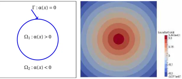
3.1 Right: schematic representation of the level set function for multi-domain problems. Left: definition of the level set function. . . 54

3.2 Right: basic level set function. Left: truncated level set function. . . 56

3.3 Filtered level set function and interface refinement using anisotropic mesh adaptation. . . 58

3.4 Characteristic length for isotropic and anisotropic element based on a clas-sical formula . . . 66

(11)

3.5 Set up of the 2D dam break . . . 67

3.6 Column fall evolution and refined meshes . . . 68

3.7 Non-dimensional front position evolution . . . 68

3.8 Non-dimensional column height evolution . . . 69

3.9 Set up of the 2D droplet splashing on thin liquid film . . . 70

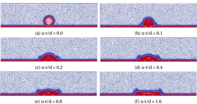
3.10 Meshes evolution for the droplet splashing on a thin film at Re = 20, We = 2000 70 3.11 Evolution of the zero-isovalue of the level set for the droplet splashing on a thin film at Re = 20, We = 2000. . . 70

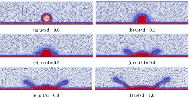
3.12 Meshes evolution for the droplet splashing on a thin film at Re = 100, We = 2000 . . . 71

3.13 Evolution of the zero-isovalue of the level set for the droplet splashing on a thin film at Re = 100, We = 2000 . . . 71

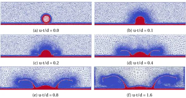
3.14 Meshes evolution for the droplet splashing on a thin film at Re = 1000, We = 2000 . . . 72

3.15 Evolution of the zero-isovalue of the level set for the droplet splashing on a thin film at Re = 1000, We = 2000 . . . 72

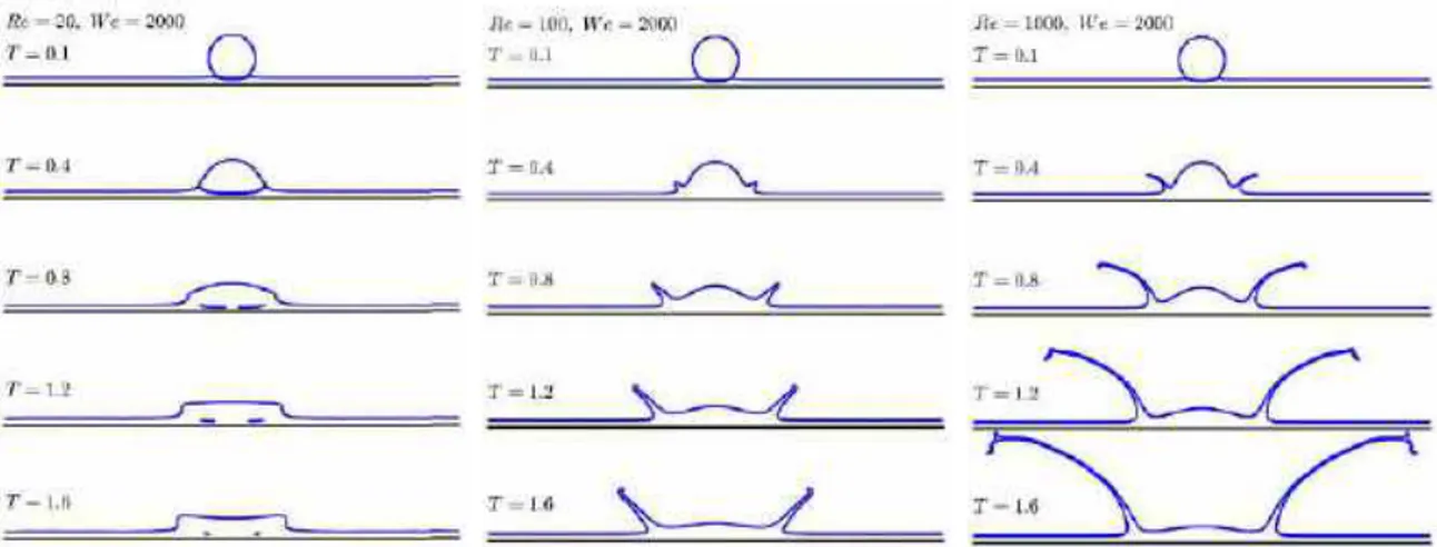
3.16 Evolution of the instantaneous interface for the droplet splashing on a thin film for the different Reynolds numbers, adopted from the work of [62] . . . 73

3.17 Set up of the 2D rising bubble . . . 73

3.18 2D rising bubble evolution . . . 74

3.19 Refined meshes for the 2D rising bubble . . . 75

3.20 Set up of the 3D simulations of the axisymetric and non-axisymetric merg-ing of two bubbles . . . 75

3.21 Comparison between the experimental measurement of [66] and the simu-lation for the co-axial coalescence of two bubbles . . . 76

3.22 Comparison between the experimental measurement of [66] and the simu-lation for theoblique coalescence of two bubbles . . . 77

3.23 Evolution of the refined meshes the 3D bubble shape for the co-axial coa-lescence . . . 78

3.24 Evolution of the refined meshes the 3D bubble shape for the oblique coales-cence . . . 79

4.1 Heat fluxes from liquid and vapor phases to interface . . . 92

4.2 Interface position for a volume of liquid that has vaporized in the time in-terval [t, t + ∆t] . . . 93

4.3 Representation of the surface tension force. . . 93

4.4 Set up of the 3D single film boiling . . . 98

4.5 Evolution of the liquid/vapor interface and meshes during 3D film boiling . 100 4.6 Evolution of the liquid/vapor interface and velocity during 3D film boiling . 101 4.7 Evolution of the temperature field and the interface location for single film boiling . . . 102

4.8 Evolution of Nu for the single film boiling in 3D . . . 103

4.9 Set up of the 3D multi film boiling . . . 103

4.10 Evolution of the liquid/vapor interface and meshes during 3D multi film boiling . . . 104

4.11 Evolution of the liquid/vapor interface and velocity during 3D multi film boiling . . . 105

4.12 Evolution of the temperature field and the interface location for multi film boiling . . . 106

(12)

4.13 Set up of the 2D quenching . . . 107

4.14 Meshes and liquid/vapor interface location at times t = 0, 1, 6, 25, 40, 60, 70, 90, 120 s . . . 108

4.15 Temperature evolution and liquid/vapor interface location at times t = 0, 1, 6, 25, 40, 60, 70, 90, 120 s . . . 109

4.16 Sensors positions inside the solid part . . . 110

4.17 Evolution of the temperature inside the solid for different positions . . . 110

5.1 General diagram for a quenching process simulation . . . 117

5.2 Division into two domains : Fluid-Solid and Solid . . . 118

5.3 Coupling scheme between Cimlib-CFD and Z-set . . . 119

5.4 Ring geometry . . . 120

5.5 Immersion of the solid geometry in the fluid domain . . . 121

5.6 Set up for the simulation of the quenching of a Ring geometry . . . 122

5.7 Evolution of the liquid/vapor interface during the boiling at times t = 0, 1, 5, 7, 8 s . . . 123

5.8 Simulation results. Temperature distribution along the sectional plane x at times t = 0, 0.15, 1, 2, 5, 7.5, 10, 12, 15 s. . . 124

5.9 Simulation restults. Contour plot of temperature distribution on the solid domain at different times t = 0, 0.15, 1, 2, 5, 7.5, 10, 12, 15 s . . . 125

5.10 Position of the thermocouples for the experimental analysis . . . 126

5.11 Comparison between experimental data and numerical results . . . 126

5.12 Position of sensors on the Ring geometry . . . 127

5.13 Cylinder head geometry . . . 128

5.14 Immersion of the solid geometry in the fluid domain . . . 128

5.15 Set up for the simulation of the quenching of a cylinder head geometry . . . 129

5.16 Simulation restults. Evolution of meshes during the boiling at times t = 0, 0.005, 0.15, 0.3, 0.5, 2 s. . . 130

5.17 Simulation restults. Evolution of the liquid/vapor interface during the boil-ing at times t = 0, 0.005, 0.15, 0.3, 0.5, 2 s . . . 131

5.18 Simulation restults. Temperature distribution along the sectional plane x at different times t =0, 0.2, 0.5, 0.7, 1, 1.2 s. . . 132

5.19 Simulation restults. Temperature distribution on the surface of the geomtry t = 0, 0.2, 0.5, 0.7, 1, 1.2 s . . . 133

5.20 Crossmember geometry . . . 134

5.21 Set up for the simulation of the quenching of the crossmember geometry. Horizontal and vertical quenching . . . 134

5.22 Evolution of the liquid/vapor interface for the horizontal quenching. . . 135

5.23 Evolution of the liquid/vapor interface for the vertical quenching . . . 136

5.24 Snapshot of the vapor field inside the solid geometry for the horizontal (left) and vertical (right) quenching taken at the same time . . . 137

5.25 Set up for the simulation of the quenching of the crossmember geometry. Horizontal quenching . . . 137

5.26 Simulation restults. Temperature distribution along the sectional plane x at different times. . . 138

5.27 Simulation restults. Temperature distribution along the sectional plane x at different times. . . 139

(13)

(14)

2.1 2D meshes used for the different transfers . . . 34

2.2 Error for the transfer from anisotropic to isotropic . . . 36

2.3 Comparison of the mass variation between both methods . . . 36

2.4 Final momentum loss in direction x . . . 39

2.5 Final momentum loss in direction y . . . 40

2.6 Final momentum loss in each direction for the 3D lid driven cavity . . . 40

2.7 Final momentum loss in each direction for the unsteady flow past a vehicule 42 2.8 Computational time speed up on the Cluster Intel . . . 43

3.1 Pourcentage of error evolution for both level set methods . . . 57

3.4 Physical parametres used for the different simulations of the 2D droplet splashing on thin liquid film . . . 69

3.5 Mass variation for the 2D rising bubble with 5000 elements . . . 74

3.6 Mass variation for the 2D rising bubble with 10 000 elements . . . 74

4.1 Physical parameters for the 3D simulation of film boiling . . . 99

4.2 Physical parameters for the 2D quenching process simulation . . . 107

5.1 Physical parametres used for first simulation of the quenching of a Ring . . 122

5.2 Physical parametres of the immersed solid while considering the phase trans-formation . . . 123

(15)

(16)

General introduction

1.1 Introduction to the industrial quenching process

Thermal Treatment describes the multifaceted operations in heating furnaces and quench-ing tanks, performed on a material in the solid state, for the purpose of alterquench-ing its mi-crostructure and properties. The output of this step is the input of all the following man-ufacturing steps such as forging, rolling processes and even the prediction of microstruc-ture evolution. Therefore, any lack of control in this upstream operation will affect the global manufacturing chain, and the consequences are then immediate such as prohibit-ing better quality, higher availability and adaptability of products. This leads to a need of improving our understanding of the involved physical phenomena, particularly for quenching processes. The modeling of the quenching process has started drawing atten-tion of many more investigators as a result of the demand of many industrials, especially the automotive, nuclear and aerospace industry. Research in both experimental and nu-merical areas and through mathematical models has proven to be effective in accelerat-ing the understandaccelerat-ing of complex problems as well as helpaccelerat-ing decrease the development costs for new processes, [1–4]. In the past, the optimization and savings in large pro-ductions were made only by large companies that could support and afford the cost of sophisticated modeling tools, specialized engineers and computer software. Nowadays, modeling has become an essential element of research and development for many in-dustrials; and realistic models of complex three dimensional quenching processes can be feasible on a personal computer. Quenching is a process that belongs to the

fam-Figure 1.1: Industrial parts and quenching in a liquid medium. Pictures taken from montupet.fr and conmecheng.com

ily of thermal treatments, the process is illustrated in Figure (1.1). The purpose of the quenching process is to give a certain micro-structure to the metal in order to achieve the required mechanical performance. This process has direct impacts on changing mechan-ical properties, controlling micro-structure and releasing residual stresses. Quenching is

(18)

a heat treatment method where a hot metal part is cooled down rapidly with the help of a quenchant such as air, water, oil, other liquids, or combinations of them. Good control of quenching is essential for correctly controlling the phase changes that take place within the alloy, and obtain the micro-structure exhibiting the desired thermomechanical prop-erties. Different parameters are controlled by the manufacturers, such as the tempering time, the chemical and thermal properties of the quenchant, or the number and the solid parts in the quenching tank. Moreover, the coolant flow structure is very important to predict heat exchanges between the solid and the hot fluid.

This Phd is done in collaboration with the company Linamar Montupet specialized in the manufacture of complex cast aluminum components for the automotive industry. They are interested in the quenching of metallic parts in liquid quenchants that can vaporize. The vaporization is generally the leading phenomenon that drives the system. Indeed, the cooling of the part is strongly conditioned by the behavior of the surrounding fluid that extracts the heat therein. The liquid determines the heat transfer at the surface of the part. Thus the study of two-phase flows with phase change, thermal transfers and fluid-solid interactions is a first step to a better understanding of quenching processes.

1.2 Physics involved in the quenching process

As explained previously, during the quenching process, an evaporation occurs at the in-terface between the hot solid part and the surrounding liquid, we call it phase change. This phenomenon is present in various industrial processes but also in natural phenom-ena such as boiling of water, condensation that creates clouds, icing of aircraft wings, etc. Each kind of phase change is characterized by triggering mechanisms induced by temper-ature or pressure variations. In the quenching process, the phase change is boiling and it is due to the metallic part that provides the required heat. Indeed, during a liquid quench-ing, the orders of magnitude between the temperatures involved are so high that the boil-ing phenomena occur durboil-ing most of the process. Thus, understandboil-ing these phenom-ena is crucial to properly control the quenching. Therefore, in order to understand the physics behind the quenching process, we must understand the different boiling modes involved. To do so, the classic approach is to consider a relative difference temperature ∆T between the hot surface and the saturation temperature of the fluid and then analyze the heat flux q at the interface between the solid and the fluid. It is common to draw the Nukiyama curve (see Figure1.2), proposed for the first time by [5], showing the heat flux as a function of the difference in temperature. It highlights the different boiling regimes of water in contact with a heated metal. As one progresses from the saturation temperature to higher temperatures, more and more bubbles appear and then merge into a vapor film, which act as a thermal insulation. As see in Figure (1.2), we can usually distinguish five boiling modes :

• The natural convection that starts before the saturation of the water, usually caused by the variation of the density of the fluid. Indeed, when the temperature gets higher, the density value decreases and on the opposite, with a lower temperature, we have a higher density. In this mode, no bubbles are yet created. It is easily mod-eled numerically, and many correlations are available in the literature to estimate the natural convection of a liquid around a hot solid.

• The partial nucleate boiling is the first step of the boiling. Small bubbles of vapor start to form on preferential sites called nucleation sites. In the case of no forced

(19)

Figure 1.2: Nukiyama curve: evolution of the surface heat flux q as a function of ∆t,[6]

convection, this is the most ordered boiling mode: bubbles form at nucleation sites and are released once critical size is exceeded. These sites are sufficiently spaced and the frequency of creation of bubbles is sufficiently small, and thus no bubble coalescence occurs.

• The fully developed nucleate boiling starts when the heat transfer is important enough so that the boiling occurs in the whole surface of the solid. In this mode, the evaporation is so important that the vapor bubbles start moving, coalesce and cre-ate unstable columns of vapor that leave the surface in a chaotic way. It is the most efficient boiling mode in terms of heat transfer. Indeed, most of the heat exchanges happen near these column of bubbles which combine evaporation and convection. • The transition boiling is a mode where boiling is so important that in some regions, a partial vapor film start to create, blocking the contact between the liquid and the solid part. This degrades the heat transfer, which results in a negative slope on the curve from Nukiyama. This mode generally does not last long during the quenching process.

• The film boiling is a mode where a continuous vapor film covers the entire hot sur-face of the solid part. The relative difference temperature is so high that the vapor-ization takes place directly at the interface between the film and the liquid. This film has an isolating effect, thus greatly limiting the heat transfer between the liq-uid and the solid part. This mode starts at the minimal temperature Tmi n= 100◦C

(20)

also called Leidenfrost temperature, which refers to the Leidenfrost effect. It is the phenomenon of calefaction that appears when a drop is placed on a hot plate: the vapor film thus created makes it "levitate" above the plate for a time that can be quite long (more than a minute depending on conditions).

In the case of industrial applications, nucleate boiling represents the most efficient boil-ing heat transfer regime. In quenchboil-ing processes, the temperature is considerably larger than the Leidenfrost temperature. Thus, a vapor film surrounds instantaneously the part and prevents it from cooling.

1.3 Brief literature on the quenching process

In order to give an idea of the evolution of the numerical modeling of the quenching pro-cess, a brief literature review will be presented here. Major influencing factors such as the design of the quenching tank, the complexity of the solid geometry, the location of the solid part in the tank and the surface state of the part where pointed out in several studies,[4;7] . In the article of [8], it was discussed that the kind of quenching medium , the selection of quenching medium temperature and the selection of the medium state (unagitated, agitated) are determining factors. Indeed, the effect of agitation on the per-formance of various quenchant has been analyzed in [3;9;10], and it was shown that the agitation clearly affects the depth of the hardness of the solid part, since it is partly re-sponsible of the mechanical rupture of the vapor film. On one hand, [11] pointed out that the thermal characteristics of the liquid are very important. For instance, the vaporization temperature has a direct impact on the different boiling modes. Indeed, the fluid might in some cases store more energy per unit volume, and this will increase the cooling rate since the temperature of the fluid is increased less fast; and it can be the other way around. On the other hand, in [12], it was pointed out that the thermal properties of the solid have an important influence on the boiling during the quenching process. The surface char-acteristics of the hot part such as roughness, oxidation and wettability are among those parameters. Another study in [13] showed that the orientation and the position of the hot part in the quenching tank, as well as the shape of the geometry play an important role in the quenching process. In fact, considerable differences were observed between a hor-izontal and a vertical surface in terms of behavior such as the bubble generation, growth and detachment.

In view of this brief literature review, it is clear that heat transfer during the film boiling and nucleate boiling processes during heat transfer in vaporizable liquids such as water must be as uniform as possible throughout the quenching process. This heat treatment process must take into account optimal combinations of parameters with their complex-ity in order to obtain the desired metallurgical properties such as hardness and yield strength. To this day, the physical modeling of the problem and the numerical simula-tion have proven to be a very powerful tool for predicting all the physical phenomena and controlling them thanks to the increasing performance of computational resources. For instance, the use of inverse analysis to deduce heat transfer coefficients was proposed by [11;14]. This method is called the Heat Transfer Coefficient but has its limits. This allow to simply and quickly deduce the cooling of a solid, however, without any knowledge of the fluid behavior. Moreover, it requires experiments and is not very accurate and gives no information on the underlying physics. As it was pointed out in [11;15], this method is satisfying in case of simple geometries but in an industrial context, if we consider an

(21)

experimental investigation, it remains time consuming and difficult to achieve and not so reliable. A full experimental optimization of this process is not a viable strategy due to the cost of the processes involved. Thus, it has become very important to simulate and visualize the complexity of the flows (liquid-vapor phase transition, agitation,...) and to deal with fluid-solid heat coupling. In the literature, there have been number of recent publications illustrating the enormous potential in the understanding of the quenching process through CFD (Computational Fluid Dynamics) analysis. It can be used to de-sign new and innovative quench systems with the objective of optimizing the quenching performance for distortion control and reduction of cracking problems. The author in [16] proposed a historical review of the numerical methods that have been developed to simulate the quenching process since the 80s. The work of Garwood and al. [1] was one of the first attempts to characterize a quench tank using computational fluid dynamics; they were able to predict qualitatively the main flow features in the quenchant. Others proposed to combine the flow motion with interface tracking methods to follow the evo-lution of the liquid-vapor-solid interface. For instance, [17] presented the numerical sim-ulations of a real cylinder head quench cooling process employing a new boiling phase change model; separated computational domains are constructed for the solid and liquid regions and are numerically coupled at the different interfaces. However, the modeling of the nucleation and pure convection mode is not carried out. In [18], the forced convection quenching process of hot pieces in the subcooled liquid is numerically investigated. Their method is validated and they show that there is a good agreement between the developed code and existing analytical solution and also experimental data. However, the modeling of the partial nucleate boiling is not performed and the surface tension model surface is not robust. Today, there is still room for progress in terms of modeling the quenching process.

1.4 Role of computational modeling in the design of the

quench-ing process

As explained previously, quenching is a complex thermomecanical process involving the coupling of multiple physical processes. These processes are generally multi-parameters controlled. A deviation during the quenching process has immediate consequences on the quality of the parts. Moreover, because the quality of the quench also depends on the internal shape of the parts, it is not possible to draw a general conclusion on how to perfectly quench a complex geometry. In other words, the quenching of a complex part is always a matter of compromise. This is where numerical modeling can be a great help, particularly regarding the prediction of residual stresses. A way to circumvent the need of tremendous computational resources is to identify the phenomena to simulate, with satisfactory precision and fidelity with respect to the real process. To enable the numeri-cal tool to be predictive, only phenomena with no significant impact on the results must be neglected. Thus, the major factor to be considered in the modeling of a quenching process is the phase change and the heat transfer at the interface between the solid and the fluid, see Figure 1.3. To study and optimize a quenching process, the heat transfer in the quenching tank has to be modeled in the same way of a real situation as closely as possible. Given the geometry of the solid part, different boundary conditions, fluid com-position and properties and other complexities, an analytical solution in not feasible and computational modeling has to be resorted to. Over the last 20 years, CFD has gained its reputation of being an efficient tool in identifying and solving such problems. The tools

(22)

Figure 1.3: Schematic representation of the quenching process

used in this thesis are the Finite Element Method (FEM) and Computational Fluid Dy-namics (CFD). This method is shown as an attractive way to solve turbulent flows and heat transfers and it can be applied for a variety of solid geometry and boundary condi-tions. The main process is detailed in the flowchart presented in Figure (2.4).

1.5 Objectives of the thesis

As explained previously, although computational fluid dynamics are being used increas-ingly in quenching tank design, there is still considerable imprecision due to assumptions that must be made in particular the use of simple geometries and approximated quench-ing environment. Today, there is a strong demand from many industrial companies to control this heat treatment process taking into account optimal combinations of param-eters with their complexity in order to obtain the desired metallurgical properties such as hardness and yield strength. Thus, the objective of this thesis is to set a numerical frame-work able to simulate the quenching process at an industrial scale. In this thesis, two main aspects will be studied, analyze and simulate the liquid-vapor-solid interactions and the implementation of the coupling between two codes (Cimlib-CFD and Z-set). The results coming from these numerical development will be validated by confrontations with the experiments proposed in agreement with the company Linamar Montupet.

Due to the complexities of the physics that may occur for such application, the modeling of the fluid-solid interaction is not straightforward. The proposed numerical method for modeling such multiphase applications (gas/fluid/solid) will be referred as the immersed volume method (IVM). It allows an improved, simple and accurate resolution; in partic-ularly at the interface between the fluid and solid. This method simplifies considerably the geometric definition and the resolutions, and has been widely used for multiphase applications. The direct numerical simulation of multiphase flows with phase change re-quires the use of a method to locate the liquid/vapor interface. In fact, to locate each interface, a signed distance function called level set is used, this approach is defined as a monolithic approach since it consists in solving a single set of equations for the whole computation domain, and this will allows to take into all the different scales of the prob-lem ; from the millimeter of the vapor bubble to the meter of the complex geometries. The first step towards a more accurate framework is to focus on evaluating and then

(23)

improv-Solid :

dimension, position, material properties

Fluid:

properties, initial temperature

Initial and boudary conditions

Numerical models:

Phase change and surface tension

Resolution:

Fluid and solid temperature, and velocity

Results and post processing: Temperature and velocity profiles

t ≥ tf i nal?

(24)

ing the existing level method : the presence of strong thermal gradients at the interface, these equations are not dubious of the resolution by stabilized element which ensures the good convergence of the solution. A full description and details about this method will be given. Furthermore, the immersed volume method is combined with an anisotropic mesh adaptation technique to ensure an accurate capture of the different interfaces. The use of a well adapted mesh along the interfaces ensures an accurate distribution of the thermo-mechanical parameters over the computational domain. The mesh is anisotropic and well adapted along the fluid/solid interfaces and isotropic with a relatively small back-ground mesh size in the rest of the domain.

Despite the considerable advances in computational fluid dynamics (CFD) and the in-creasing computer power, different challenges still need to be addressed for providing ac-curate and efficient simulations. The problem can be cast as a thermal fluid-structure in-teraction one involving the simultaneous resolution of turbulent flows with phase change and conjugate heat transfers between the solid and the fluid subdomains. Indeed, this framework must take into account turbulent boiling (with or without agitators), phase change natural and forced convection and therefore the complexity of industrial cases with a high thermal gradient. The industrial objective will therefore be to characterize the various boiling regimes observed under transient conditions, to precisely measure the associated heat transfer, to couple the thermal field and finally to be able to control the cooling rate of the process. Indeed, it becomes necessary, for a complete quenching sim-ulation to take into account more precisely the evolution of the liquid and vapor phases: heating regime, nucleate boiling regime and convection regime. Finally, it is important to mention that classical Finite Element methods to solve the unsteady Navier-Stokes and heat transfer equations suffer from lack of stability, in particular at high Reynolds and Peclet numbers. These sources of numerical difficulties have been treated using different approaches and these finite element solvers are already implemented in our library. In the case of the quenching process, the phenomena studied concern both the phase change at small scales (germination and growth of a vapor bubble) and the boiling phe-nomena at large scales occurring during the quenching but also the phase transformation of the treated part and the residual stresses. Residual stresses developed after quench-ing of alloys cause distortion durquench-ing subsequent machinquench-ing. As a result, machined parts may be out of tolerance and have to be cold worked or re-machined. Experimental mea-surement of residual stresses is lengthy, tedious and very expensive. Thus,a simulation that takes into account the phase transformation inside the solid is mandatory; this is the second objective of the thesis. The objective of this task is to develop a generalist "gate-way" between two codes capable of accurately transferring fields from a fluid-structure mesh to a structure mesh. This structure mesh will be used in the software Z-set to per-form residual stress analysis. Several interpolation techniques of the fields (temperature, flux, etc ...) exist in the literature. In our library, we use only 2D triangular elements and tetrahedral elements in 3D. The implemented interpolation method must be robust and optimal in terms of computational time, works in parallel on multiple cores and most importantly, must be conservative. Note that the interpolation is not only used for the coupling, but most of all, during the anisotrpic adaptation procedure. And recall that in multiphase applications, the mesh adaptation is user every time step. An improvement on the linear interpolation method will therefore be proposed. Finally, to validate and to asses the performance of the developed framework, experimental data will be provided by the industrial partner and the numerical validation of the new complete quenching

(25)

model will be done. The complexity of the geometry, the calculation time, the flexibility for the implementation of the simulations, taking into account the complete quenching tank with the entry and the exit of water to maintain the temperature of the quench tank, the test coupling with Z-set, taking into account the phase transformation and the resid-ual stresses, will form all points of interest in this task.

To sum up, all these following tasks have been achieved:

• Develop advanced numerical methods to describe the interfaces liquid/vapor/solid • Couple the multiphase flows with the convection-diffusion-reaction equations to

model the phase change at the liquid-vapor interface

• Use the latest development on the mesh adaptation procedure and parallel compu-tation to handle large complex industrial simulations

• Conservative interpolation between unrelated unstructured meshes and coupling between two codes

• Validate the numerical framework by comparison with the experimental data pro-vided by real quenching simulations propro-vided by the industrial partner Linamar Montupet

To summarize, the originality of this work lies in the simulation of realistic industrial con-ditions and quenching devices, and robustness by limiting the assumptions made and restraining non-physical use of quenching parameters. All those elements represent the features dedicated to industrial abilities of the framework.

1.6 Work environment

In this thesis, all the numerical implementations of the developed methods are carried out using the finite element library Cimlib-CFD; which stands for CIM as Advanced Comput-ing in Material formComput-ing research group and LIB for library and CFD, computational fluid dynamics. It is developed by the CFL team which stands for Computers and Fluids. It is the base for different numerical applications developed at CEMEF (www.cemef.mines-paristech.fr), in collaboration with other research teams and industrial partners. This scientific library represents an Object Oriented Program and a fully parallel code, writ-ten in C++, gathers the numerical development of the group (Ph.D. students, researcher, associate professor. . . ). Cimlib-CFD aims at providing a set of components that can be organized to build numerical simulation of different industrial processes and the present one is the simulation of the quenching process for the company Linamar Montupet.

1.7 Author’s contribution during the PhD

The contributions of the author in terms of publications, oral communications and prizes are presented below.

(26)

1. Bahbah, C., Mesri, Y., & Hachem, E. Interpolation with restrictions in an anisotropic adaptive finite element framework. Finite Elements in Analysis and Design, 2018, 142, 30-41.

2. Bahbah, C., Khalloufi, M., Larcher, A., Mesri, Y., Coupez, T., Valette, R., & Hachem, E. Conservative and adaptive level-set method for the simulation of two-fluid flows. Computers & Fluids, 2019, 191.

3. Bahbah, C. & Hachem, E. Fluid-solid coupling for simulating the temperature evolu-tion during the quenching process. In progress

Communications

1. Bahbah, C., Mesri, Y., & Hachem, E. Éléments finis adaptatifs pour la simulation des phénomènes interfaciaux avec changement de phase. 13ème Colloque National en Calcul des Structures, France 2017.

2. Bahbah, C., Mesri, Y., & Hachem, E. Interpolation with restrictions in an anisotropic adaptive finite element framework for CFD applications. International Workshop on Complex Turbulent Flows, Morocco 2017.

3. Bahbah, C. & Hachem, E. Accurate Adaptive Eulerian Framework for Liquid-gas-solid interactions. Fluids and Complexity, France 2018.

4. Bahbah, C., Khalloufi, M., Mesri, Y., & Hachem, E. Accurate Adaptive Eulerian Frame-work for Liquid-gas-solid interactions. 13th World Congress on Computational Me-chanics (WCCM XIII), USA 2018.

5. Bahbah, C. & Hachem, E. Accurate Adaptive Eulerian Framework for Liquid-gas-solid interactions. UCA Complex days, France 2019.

Awards

1. Price for the best poster in the session numerical modeling for multiphysics, Con-ference CSMA 2017.

2. Finalist of the Pierre Laffitte medal 2018. The medal was created in the honor of the Professor Pierre Laffitte who was the former director of MINES ParisTech (1972-1984) and senator of the region Alpes Maritimes in France (1995 – 2008).

1.8 Layout of the thesis

The thesis is divided into six chapters. Chapter 1 is an introduction to the topic consid-ered in this thesis. Chapter 2 is dedicated to the Eulerian conservative framework; the Immersed Volume Method (IVM) coupled to the mesh adaptation technique and a newly developed parallel conservative interpolation method are presented. In Chapter 3, we present the moving interface capturing method to follow the evolution of the different in-terfaces in multiphase flows. A new definition of the level set function is presented and special attention is given to stabilization methods for solving the Navier-Stokes equations. The mathematical modeling of the phase change at the interface as well as the stabilized finite element used for solving the conjugate heat transfer are detailed in Chapter 4. The coupling between our code Cimlib-CFD and the software Z-set is explained in Chapter

(27)

6. The validation of the framework on some industrial applications is also detailed in the second part of this chapter. The computation of different benchmarks tests has been also carried out and several comparisons with experimental works will be also presented along this manuscript. Finally, in the last chapter, conclusion and the possible extension of the present work to include more features is explored.

1.9 Résumé du chapitre en français

Ce chapitre d’introduction nous permet d’abord de présenter une description générale autour des enjeux industriels et numériques liés au procédé de trempe. La trempe est une méthode de traitement thermique où un métal chaud est refroidi rapidement à l’aide d’un medium tel que l’air, l’eau, l’huile ou d’autres liquides ou de combinaisons de ceux-ci. Il a pour but de donner au métal une certaine microstructure afin d’atteindre les per-formances mécaniques requises. Ce procédé a des impacts directs sur l’évolution des propriétés mécaniques, le contrôle de la microstructure et la libération des contraintes résiduelles. Afin de réaliser un procédé optimal, il est essentiel de contrôler correctement les transformations de phase qui ont lieu dans l’alliage, et ainsi obtenir la microstruc-ture présentant les propriétés thermomécaniques souhaitées. Différents paramètres sont contrôlés par les fabricants, comme le temps de trempe, les propriétés chimiques et ther-miques du medium, ou le nombre de pièces solides dans le réservoir de trempe.

Cette thèse est réalisée en collaboration avec la société Linamar Montupet spécialisée dans la fabrication de composants complexes en aluminium pour l’industrie automo-bile. Ils s’intéressent à la trempe des pièces métalliques dans les medium liquides pou-vant vaporiser. La vaporisation est généralement le principal phénomène qui anime le système. En effet, le refroidissement de la pièce est fortement conditionné par le com-portement du fluide environnant qui extrait la chaleur provenant de la pièce chaude. Le liquide détermine la transfert de chaleur à la surface de la pièce. Ainsi, l’étude des écoule-ments multiphasiques à changement de phase, des transferts thermiques et des interac-tions fluide-solide est un premier pas vers une meilleure compréhension des procédés de trempe. En effet, durant le procédé de trempe, une évaporation se produit à l’interface entre la partie solide chaude et le liquide environnant, on parle de changement de phase. Ce phénomène est présent dans divers procédés industriels, mais également dans des phénomènes naturels tels que l’ébullition de l’eau, la condensation qui crée des nuages, le glaçage de ailes d’avion, etc. Chaque type de changement de phase est caractérisé par des mécanismes de déclenchement induits par des variations de température ou de pres-sion. Dans le processus de trempe, le changement de phase est l’ébullition et il est dû au solide qui fournit la chaleur requise. En effet, lors d’une trempe liquide, les ordres de grandeur entre les températures en jeu sont si élevés que les phénomènes d’ébullition se produisent pendant la majeure partie du processus.

L’analyse bibliographique a permis de constater que les informations sur l’ébullition tran-sitoire ne sont pas complètes. En effet, il est connu qu’une fois l’ébullition déclenchée, ce sont les bulles qui sont principalement responsables du transfert de la chaleur de la paroi vers le liquide. Le diamètre des bulles, la fréquence de détachement et la densité des sites de nucléation sont donc importants. À faible surchauffe ou faible densité de flux, les bulles sont formées à partir de quelques sites de nucléation uniquement. Ce régime s’appelle « régime de bulles isolées ». Au transfert par convection dans le liquide hors de la zone d’influence des bulles, s’ajoute le transfert thermique dû aux bulles. Les bulles

(28)

naissent à la paroi, grandissent et se détachent et leur cycle de vie améliore les échanges thermiques. Aux deux mécanismes mentionnés, un troisième peut être ajouté, il s’agit de l’évaporation de la microcouche qui existe au pied de la bulle ou ébullition nuclée. Une optimisation expérimentale complète de ce processus n’est pasune stratégie viable en raison du coût des processus impliqués. Bien que la dynamique des fluides soit de plus en plus utilisée dans la conception des réservoirs de trempe, le manque de précision est toujours un problème majeure en raison des hypothèses qui doivent être faites en amont ; particulier l’utilisation de géométries simples et d’un environnement de trempe très ap-proximatif. L’amélioration et le contrôle de ce procédé suscitent un intérêt grandissant et deviennent un axe majeur de progrès pour les industriels.

L’objectif scientifique de ce projet de thèse est d’étendre le premier modèle de trempe pour passer de l’échelle académique à l’échelle industrielle tout en prenant en compte l’ébullition turbulente (avec ou sans agitateurs), le changement de phase, convection na-turelle et forcée et donc la complexité des cas industriels à fort gradient thermique et finalement de confronter les nouveaux développements aux expériences proposés en ac-cord avec Montupet. L’objectif industriel sera donc de caractériser les différents régimes d’ébullition observés, de mesurer précisément les transferts thermiques associés, de cou-pler le champ thermique, et finalement de pouvoir contrôler la vitesse de refroidissement du procédé. En effet il devient nécessaire, pour une simulation complète de trempe, de retravailler les solveurs numérique existants pour prendre en compte plus précisément l’évolution des phases liquide et vapeur : régime de caléfaction, régime d’ébullition nu-cléée et régime de convection. Les phénomènes étudiés concernent aussi bien la transfor-mation de phase de la pièce traitée et les contraintes résiduelles, le changement de phase aux petites échelles (germination et croissance d’une bulle de vapeur) et les phénomènes d’ébullitions aux grandes échelles intervenant lors de la trempe. En se basant sur les outils existants au sein de la librairie de calcul élément finis de l’équipe Calcul Intensif et Mécanique des Fluides (CFL) du Centre de Mise en Forme des Matériaux (CEMEF) de l’école des Mines de Paris (Mines ParisTech), nous avons identifié les nouveaux be-soins numériques. La méthode d’imersion de volume (IVM) développée par l’équipe CFL est adoptée pour prendre en compte les interactions fluide/structure et la distribution des propriétés thermo-mécaniques. Maintenir un bon niveau de précision nécessite un maillage très fin, ainsi l’adaptation de maillage anisotrope est utilisée, ce qui permet une résolution fine des physiques aux interfaces. Ainsi, dans cette thèse, deux aspects prin-cipaux seront étudiés: analyser et simuler les interaction liquide-vapeur-solide et mettre en œuvre le couplage entre deux codes (Cimlib-CFD et Z-set) afin de prendre en compte la transformation de phase au sein du solide. Pour ce faire, ces différentes tâches ont été réalisées :

• Développer des méthodes numériques pour décrire les interfaces liquide/gaz/solide • Coupler les écoulements multiphasiques avec la thermique pour le changement de

phase (liquide/gaz)

• Utiliser les derniers travaux sur l’adaptation de maillage et calcul parallèle pour traiter des cas à l’échelle industrielle

• Interpolation conservative des champs entre deux maillages et couplage entre deux codes

• Valider les résultats numériques par des confrontations avec des résultats expéri-mentaux en collaboration avec Linamar Montupet.

(29)

En résumé, l’originalité de ce travail réside dans la simulation de conditions industrielles et de dispositifs de trempe réalistes. Ce nouveau framework permet l’optimisation et le contrôle de ce procédé, ce qui représente un axe majeur de progrès pour les industriels.

1.10 Bibliography

[1] D. Garwood, J. Lucas, R. Wallis, J. Ward, Modeling of the flow distribution in an oil quench tank, Journal of Materials Engineering and Performance 1 (6) (1992) 781– 787. 2,6

[2] D. M. Wang, A. Alajbegovic, X. Su, J. Jan, Numerical simulation of water quenching process of an engine cylinder head, in: ASME/JSME 2003 4th Joint Fluids Summer Engineering Conference, American Society of Mechanical Engineers Digital Collec-tion, 2003, pp. 1571–1578.

[3] F. Lemmadi, A. Chala, S. Ferhati, F. Chabane, S. Benramache, Structural and mechan-ical behavior during quenching of 40crmov5 steel, Journal of Science and Engineer-ing 3 (1) (2013) 1–6. 5

[4] C. ¸Sim¸sir, C. H. Gür, A simulation of the quenching process for predicting tempera-ture, microstructure and residual stresses., Strojniski Vestnik/Journal of Mechanical Engineering 56 (2). 2,5

[5] S. Nukiyama, The maximum and minimum values of the heat q transmitted from metal to boiling water under atmospheric pressure, International Journal of Heat and Mass Transfer 9 (12) (1966) 1419–1433. 3

[6] V. Dhir, Boiling heat transfer, Annual review of fluid mechanics 30 (1) (1998) 365–401.

v,4

[7] P. Cavaliere, E. Cerri, P. Leo, Effect of heat treatments on mechanical properties and fracture behavior of a thixocast a356 aluminum alloy, Journal of Materials Science 39 (5) (2004) 1653–1658. 5

[8] B. Taraba, S. Duehring, J. Španielka, Š. Hajdu, Effect of agitation work on heat trans-fer during cooling in oil isorapid 277hm, Strojniški vestnik-Journal of Mechanical Engineering 58 (2) (2012) 102–106. 5

[9] J. Olivier, B. Clement, J. Debie, F. Moreaux, Stirring of quenchants fluids: design con-siderations and metallurgical consequences, Trait. Therm 206 (1986) 29–42. 5

[10] N. Chen, L. Han, W. Zhang, X. Hao, Enhancing mechanical properties and avoid-ing cracks by simulation of quenchavoid-ing connectavoid-ing rods, Materials Letters 61 (14-15) (2007) 3021–3024. 5

[11] A. Buczek, T. Telejko, Investigation of heat transfer coefficient during quenching in various cooling agents, International Journal of Heat and Fluid Flow 44 (2013) 358– 364. 5

[12] S. A. Ebrahim, S. Chang, F.-B. Cheung, S. M. Bajorek, Parametric investigation of film boiling heat transfer on the quenching of vertical rods in water pool, Applied Ther-mal Engineering 140 (2018) 139–146. 5

(30)

[13] N. Kaneyasu, F. Yasunobu, U. Satoru, O. Haruhiko, Effect of surface configuration on nucleate boiling heat transfer, International Journal of Heat and Mass Transfer 27 (9) (1984) 1559–1571.5

[14] P. Archambault, S. Denis, A. Azim, Inverse resolution of the heat-transfer equation with internal heat source: Application to the quenching of steels with phase trans-formations, Journal of materials engineering and performance 6 (2) (1997) 240–246.

5

[15] G. Ramesh, K. N. Prabhu, Assessment of axial and radial heat transfer during immer-sion quenching of inconel 600 probe, Experimental Thermal and Fluid Science 54 (2014) 158–170. 5

[16] D. S. Mackenzie, History of quenching, International Heat Treatment and Surface Engineering 2 (2) (2008) 68–73.6

[17] V. Srinivasan, K.-M. Moon, D. Greif, D. M. Wang, M.-h. Kim, Numerical simulation of immersion quenching process of an engine cylinder head, Applied Mathematical Modelling 34 (8) (2010) 2111–2128.6

[18] H. Ramezanzadeh, A. Ramiar, M. Yousefifard, Numerical investigation into coolant liquid velocity effect on forced convection quenching process, Applied Thermal En-gineering 122 (2017) 253–267.6

(31)

(32)

Eulerian conservative and adaptive

framework

2.1 Introduction

In recent years, there have been increasing interest in studying numerically a variety of engineering applications that involve thermal coupling of fluids and solids. However, the modeling and simulation of fluid-solid interactions (FSI) of multiphase applications are considered challenging since they involve the study of the interactions between a solid body and its surrounding media or the interactions between different fluid flows. In this thesis, we are interested in the numerical simulation of thermal coupling problems in-volving multiphase flows. The most common trend to deal with multi-component do-mains is issued from the body fitted approach whereby the global domain is partitioned into several local subdomains over each of which a local model is solved [1]. However, during the assembly, the coordination between the meshes can become complicated or even sometimes infeasible.

Immersed methods can be considered as a good tool for reducing the computational cost induced by body-fitted approaches and overcoming the interface treatment step required by non-body fitted techniques. They simplify a number of issues in multiphase applica-tions such as meshing the fluid domain, the use of a fully eulerian algorithm, dealing with complex geometries in terms of curvatures, sharp angles and singularities and topological changes. We can find in the literature three classes of methods for immersing geometries into a computational domain. The first group gathers the methods that enrich the nu-merical solution’s space in a finite element framework [2]. These methods avoid the com-putational cost needed to construct a mesh that is well representative of the immersed bodies but requires the modification of the finite element solvers.

The second accounts for the effect of the immersed objects by introducing an additional source term into the governing equations, [3–5]. However, when dealing with multi-physical domains, these methods can rapidly become very expensive and time-consuming. The interface tracking methods constitute a third class of immersion; they propose a dif-ferent scenario than the previously mentioned techniques [6]. The main idea is to retain the use of the monolithic formulation and coupling it to some additional features that could allow a better and accurate resolution, in particularly at the interface between the fluid and solid. Recall that the monolithic resolution is based on the level set approach and consists in considering a single mesh for all components; fluid and solid domains. The interfaces between the different multiphysical domains are tracked by signed dis-tance functions called level set. The immersed volume method (IVM) [6–10] was defined in that sense and can be applied on a wide range of multimaterial applications. The three main ingredients of the immersed volume methods are : (i) the level set, a signed distance function that is used to localize and immerse the solids inside the global domain, (ii) then an anisotropic mesh adaptation is employed to provide a good capture of the interfaces between the solid and fluid parts, (iii)and finally mixing the different material properties using a homogeneous distribution along the interface. The IVM method can be applied without modification for any geometry and any physical property. It can be very easily im-plemented and applied with stabilized finite element methods and in the context of mov-ing structure problems. The level set function as well as the mixmov-ing laws will be presented in the next chapter. This chapter is only dedicated to the newly developed anisotropic mesh adaptation technique coupled with a parallel conservative interpolation method.

(34)

2.2 Anisotropic mesh adaptation

In order to provide an accurate configuration of the physical problem, immersed objects should be properly defined and material properties should be well distributed. For accu-rate computations in a multiphase framework, the mesh has to be refined around the interface. Indeed, adapting the mesh to the physical behaviors and studied phenom-ena is a means to improve the accuracy of numerical results. However, difficulties might arise due to the discontinuities in the material properties between the solid and the fluid parts. In fact, when the discontinuities intersect the mesh elements arbitrarily, they will not be properly captured and hence they might result in the deterioration of the accu-racy of the solution. The objective is therefore to combine the level set representation with local mesh refinement around the zero isovalue of the level set function yielding an accurate capture of a fluid-solid interface at a low computational cost. The key to these regards is anisotropic mesh adaptation that generates highly stretched and well oriented elements allowing a good capture of sharp gradients. It implies that we can stretch the elements in certain directions according to the solution features. Several approaches to build anisotropic adaptive meshes often based on local modifications on an existing mesh can be found in the literature [11–13]. They mainly require extending the way to measure lengths following the space directions and can be done using a metric field to redefine the geometric distances. Mesh adaptation techniques based on a posteriori error estimation have also been well developed [14], leading to some standardization of the adaptation process. In this thesis, the mesh adaptation technique is based on the work [15;16], we focus on anisotropic mesh adaptation driven by directional error estimators. The mesh is dynamically adapted to the solution, i.e. velocity and interface position. The aim is to refine the discretization in the areas of the domain where the solution fields are mostly non-linear. The refinement affects both the density of elements and their shape, which is anisotropically adapted and stretched along the direction where the considered solution field is linear. The mesh becomes locally refined around the zero isovalue of the level set function which enables to sharply define the interface and to save a great number of el-ements compared to classical isotropic refinement. To do so, we start by performing an error analysis on the mesh. Then, to correlate the error with the geometry, a metric field is defined. From this metric field, an anisotropic error indicator is defined and used as a functional for a re-meshing optimization problem.

2.2.1 Edge-based error estimation

Let uhbe a P1 finite element approximation obtained by applying the Lagrange

interpo-lation operator to a regular function u ∈ C2(Ω). At each vertex i of the mesh, we have Ui = u(xi) = uh(xi) (where xi are the coordinates of the vertex i ). Let Γ(i ) be the "patch"

associated to a vertex xi of the mesh defined as the set of nodes which share one edge with xi , and let us denote by xi j the edge connecting xi to xj as seen in Figure2.1. The gradient ∇uh· xi j on the edge xi jis continuous, therefore we can write :

Uj= Ui+ ∇uh· xi j (2.1)

which leads to :

(35)

Figure 2.1: Patch Γ(i ) associated with node xi

Following the work of [16], an a posteriori error estimate based on the length distribution tensor approach and the associated edge based error analysis is defined :

|| ∇uh· xi j− ∇u(xi) · xi j||≤ max

y∈|xi_,xj_|| x

i j

· Hu(y) · xi j| (2.3)

with Huthe hessian of u. Since we want to compute the recovered gradient giof uhat the

node xi, thus we have :

∇gh· xi j= gj− gi (2.4)

The projection of the Hessian based on the gradient at the extremities of the edge is ob-tained as follows :

(∇gh· xi j) · xi j= (gj− gi) · xi j (2.5)

(Hu· xi j) · xi j= gi j· xi j (2.6)

with gi j= gj− gi. We denote the error along the edges using the following expression :

ei j=| gi j· xi j| (2.7)

This error sampling is the exact interpolation error along the edge and enables us to eval-uate the global L2error. The equation (2.7) can be evaluated only when the gradient of u is known and continuous at the nodes of the mesh, thus a recovery procedure has to be considered.

2.2.2 Gradient recovery procedure

The recovery gradient operator is defined by a local optimization problem :

Gi = ar g min

G _{j ∈Γ(i)}| (G − ∇uh) · x

i j

|2 (2.8)

Denoting by ⊗ , the tensor product between two vectors, let us introduce Xi the length distribution tensor at node i :

Xi= 1

| Γ(i ) | _{j ∈Γ(i)}x

i j

(36)

whose purpose is to give an average representation of the distribution of edges in the patch. Let us express the recovered gradient Giin terms of the length distribution tensor :

Gi = (Xi)−1

j ∈Γ(i)

Ui jxi j (2.10)

Therefore, the estimated error is thus written as :

ei j= Gi j.xi j (2.11)

Now, we seek to relate this error indicator ei j to a metric suitable for a mesh adaptation

procedure.

2.2.3 Metric construction

It is necessary to take into account the neighborhood of the node so that the best aver-aging representation is a metric defined at each node [15]. The metric can be regarded as a tensor whose eigenvalues are related to the mesh sizes, and whose eigenvectors de-fine the directions for which these sizes are applied. The metric M is a symmetric positive definite tensor representing a local base that modifies the distance computation from the Euclidean space to the metric space, therefore it takes the following expression :

˜ Mi _{= ( ˜}_Xi₎−1 _(2.12) where ˜ Xi₌ 1 | Γ(i ) | _{j ∈Γ(i)}s i j ⊗ si j (2.13)

The stretching factor si j _{of the edge i j is chosen so that the total number of nodes in}

the mesh is kept fixed. It is defined as the ratio between the original edge length and the length of the adapted edge, more details can be found in the work of jannoun2015anisotropic.

2.2.4 Mesh adaptation criterion

When simulating complex physical phenomena involving turbulent flows and heat trans-fers like the quenching process, it is highly desirable to accurately capture all the char-acteristics of the problem, including but not limited to, the flow field, the temperature variations, and the fluid/solid interfaces. Therefore, different fields can be used as a crite-rion for mesh adaptation: the adaptivity will account for the both the change of direction of the velocity, its magnitude, the level set function and the temperature field.

The common technique to derive a single metric at each node in the mesh accounting for several fields of interest relies on the rigor of computing the metrics corresponding to each of the sensor fields then performing a metric intersection operation [17]. In this work, we simplify this operation and we use one metric that accounts for different vari-ables. Therefore, based on the theory proposed in the previous section, it is possible to extend the definition to account for several sources of error. Thus, the following vector of sources of error is defined:

v(xi) = Vi | Vi|, | Vi | maxj| Vj | , Ti Tmax, φ max(φ) (2.14)

(37)

Because all fields are normalized (the velocity components vx,vy and vzby the local

ve-locity norm, the veve-locity norm and the level set function by their respective global maxi-mum), a field that is much larger in absolute value does not dominate the error estimator, and the variations of all variables are fairly taken into account.

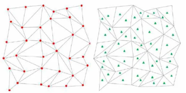
In the framework of the immersed volume method, the goal is to provide a good repre-sentation of the fluid/solid interfaces for a fixed number of nodes in the mesh. Let us consider the example of two immersed solid bodies. Starting from a isotropic mesh, we generate the multidomain metric and we adapt the mesh to this metric. After several iter-ations, one can clearly see from Figure2.2that the interface between these objects and the surroundings is well adapted. Figure2.3clearly shows that the refinement at the interface

(a) Initial mesh (b) Final mesh

Figure 2.2: Mesh adaptation algorithm applied to two immersed bodies

is anisotropic. The nodes are highly condensed in the vicinity of the interface favoring its accurate capture. This validates how the developed algorithm optimizes the distribution of the nodes to produce a sharp anisotropic mesh that is well adapted based on a given variable (here, the level set function of the immersed solids). Note also, when using an anisotropic mesh, with elements stretched in a ’right’ direction, one could allow not only to save a lot of elements but also to well describe the geometry in terms of curvature, angles, etc. An important point to mention here is that this mesh adaptation technique works under the constraint of a fixed number of nodes. With such an advantage, we avoid a drastic increase of mesh complexity and hence computational cost when dealing with complex CFD problems. However, one serious drawback of many mesh adaptivity algo-rithms on unstructured meshes the necessity of interpolating solutions fields from the initial mesh to the newly adapted mesh. Such interpolation may destroy conservation of important physical quantities and leads to errors in the solution fields. Thus, in the next section, we will give a brief review of the several conservative interpolation methods that can be found in the literature and give details on the conservative interpolation algorithm implemented in this work.