Stabilité des paires de tourbillons contra-rotatifs: application au tourbillon de jeu dans les turbomachines

(1)

HAL Id: pastel-00005529

https://pastel.archives-ouvertes.fr/pastel-00005529

Submitted on 24 Nov 2009

HAL is a multi-disciplinary open access

archive for the deposit and dissemination of sci-entific research documents, whether they are pub-lished or not. The documents may come from teaching and research institutions in France or abroad, or from public or private research centers.

L’archive ouverte pluridisciplinaire HAL, est destinée au dépôt et à la diffusion de documents scientifiques de niveau recherche, publiés ou non, émanant des établissements d’enseignement et de recherche français ou étrangers, des laboratoires publics ou privés.

Stabilité des paires de tourbillons contra-rotatifs:

application au tourbillon de jeu dans les turbomachines

Vincent Brion

To cite this version:

Vincent Brion. Stabilité des paires de tourbillons contra-rotatifs: application au tourbillon de jeu dans les turbomachines. Engineering Sciences [physics]. Ecole Polytechnique X, 2009. English. �pastel-00005529�

(2)

THÈSE DE DOCTORAT

DE L’ÉCOLE POLYTECHNIQUE

présentée par

Vincent Brion

pour obtenir le titre de

Docteur de l’Ecole Polytechnique

Spécialité : Mécanique

Stabilité des paires de tourbillons contra-rotatifs:

application au tourbillon de jeu dans les turbomachines

soutenue le 7 octobre 2009

devant le jury composé de :

M. P. Brancher

M. G. Casalis

M. L. Jacquin

Directeur de thèse

M. F. Leboeuf

M. T. Leweke

Rapporteur

M. M. Rossi

Rapporteur

M. P. J. Schmid

(3)

(4)

Résumé

La stabilité du tourbillon de jeu d’aubage dans les compresseurs est étudiée au travers d’un modèle équivalent de paires de tourbillons. L’objectif consiste à contrôler ce tourbillon en excitant ses instabilités hydrodynamiques, ce qui permettrait de le dissiper plus rapidement et d’augmenter les performances des turbomachines.

La première partie est dédiée à l’étude théorique des instabilités dans les paires de tourbil-lons. Un mode instable 2D du dipôle de Lamb-Chaplygin est d’abord présenté. On s’intéresse ensuite aux instabilités 3D, et à leur contrôle. Les instabilités de Crow et de Widnall, notamment avec champ de vitesse axial, sont calculées. L’utilisation d’un code de perturbation optimale permet ensuite d’optimiser la croissance de ces instabilités, ce qui fait apparaître l’importance des points de stagnation hyperbolique dans les croissances transitoires, et des possibilités de contrôle prometteuses pour les sillages d’avion de transport.

Le tourbillon de jeu est ensuite étudié en soufflerie, grâce à un montage permettant, dans une première configuration, de générer une paire de tourbillons tandis qu’une deuxième con-figuration, grâce à l’introduction d’une plaque séparatrice, génère un tourbillon en interaction avec la paroi. L’étude de l’écoulement moyen montre que la plaque plane modifie fortement le comportement du tourbillon. En ce qui concerne les instationnarités, l’instabilité de Crow est détectée dans le cas sans plaque mais pas dans le tourbillon avec plaque, ce qui semble indiquer que la paroi inhibe cette instabilité.

Mots clés : turbomachine, tourbillon, jeu, stabilité hydrodynamique, Crow, Widnall, per-turbation optimale, point hyperbolique, Particle Image Velocimetry, fil chaud, sonde de pression 7 trous, contrôle, soufflerie.

Abstract

The stability of the tip leakage vortex in compressors is investigated through the model of vortex pairs. The goal is to control this vortex by boosting its hydrodynamic instabilities, in order to mitigate it more rapidly with the surrounding flow and increase performances of turbomachines.

The first part is dedicated to the theoretical study of instabilities in vortex pairs. A 2D unstable mode of the Lamb-Chaplygin dipole is presented. We then focus on the 3D instabilities, namely Crow and Widnall, with and without axial flow. An optimal perturbation algorithm is used in order to optimize the growth rate of these instabilities. We find that the hyperbolic stagnation points play a major role in the transient growth of energy, and that interesting possibilities exist to control aircraft trailing vortices.

The tip leakage vortex is then investigated in a wind tunnel, with an apparatus enabling two configurations. The first configuration produces two opposed and equal vortices while the second one, with a splitter plate, produce one vortex that interacts with the wall. The study of the mean flow shows that the wall modifies significantly the behaviour of the vortex. The Crow instability is detected without the splitter plate only. This suggests that the wall prevents the development of the Crow instability.

Keywords : turbomachinery, vortex, clearance, hydrodynamics stability, Crow, Widnall, optimal perturbation, hyperbolic point, Particle Image Velocimetry, hot-wire, 7-hole pressure probe, control, wind tunnel.

(5)

Remerciements

De longues années de thèse, beaucoup de personnes formidables rencontrées en chemin, et des souvenirs inoubliables . . .

Merci à Denis Sipp de m’avoir accueillit dans son unité, de m’avoir lancé sur les tourbillons, et d’avoir partagé avec moi ses bonnes idées. Le projet côté soufflerie a pu être mené à bien grâce au concours d’un grand nombre d’acteurs, que je tiens à remercier vivement : François Lambert, qui a dessiné le montage d’après un cahier des charges difficile, Jean-Pierre Tobeli, qui a redémarré la soufflerie de zéro, Jean-François Pulizzi et Michel Agrapart, qui ont par un tour de main incroyable, réussi à monter la maquette et ses appendices en veine, Michel Vegran, Philippe Huet, Pascal Audo, les spécialistes des rafales, Jean-Marc Luyssen et Didier Coponet, Michel Gouhier de S3 pour les bouillies, la laser team, et les rois de l’expérimentation, Gilles Losfled et François Becavin, Didier Soulevant, Nicolas Severac pour la bonne ambiance de S5, Patrik Servel et Michel Erard pour leur soutien informatique. Je n’oublie pas Philippe Mourer qui a supervisé la fabrication du montage à l’atelier central.

Je ne compte pas les heures passées en soufflerie en compagnie de Michel Alaphilippe. Il m’est impossible de lui rendre ici tout ce qu’il m’a apporté. Je crois tout simplement que sans lui je n’aurais pas fait le dixième de ce que j’ai fait. Témoin de mes galères et de mon enthousiasme, compagnon de solitude, il a marqué mon séjour ici.

Ma thèse aurait été beaucoup plus triste aussi si je n’avais pas partagé beaucoup d’excellents moments avec les autres personnes du département. Je lance un immense merci à Serge Petit et à Florence Bouvier pour leur humour décapant. Je dois beaucoup également au temps passé avec Guy Rancarani, Claire Planchard, Yves Lesant, Marie-Claire Merienne, Corinne de Pablo, Angélique Baudelot, Dominique Grandson et Kurita Mitsuru, qui a décoré d’une joyeuse teinte japonaise ma dernière année ici.

La course à pied dans le bois de Meudon a été un vrai bonheur hebdomadaire. J’adresse donc ici ma profonde gratitude à Sébastien Girard, Yves Carpels, Thierry Pot, Jean-Paul Antony, Benjamin Leclaire, Yves Carpels, Pascal Molton et Gérald Courant. Ils ont été des compagnons d’effort extraordinaires.

J’adresse un merci très ému à tous mes proches compagnons de thèse. Ils m’ont beaucoup apporté et je n’oublierai pas de si tôt la franche camaraderie qui a régné ici. Un grand merci donc à Bruno Mangin, Paul Quantin Elias, Philippe Meliga, Benoît Gardarin, Olivier Marquet, Benjamin Leclaire, Samuel Davoust et Hugues Dekerret. Un grand merci également à Sarah Benbaba qui a su me supporter dans le bureau ces deux dernières années. Et puis je remercie aussi les autres stagiaires que j’ai eu le plaisir de rencontrer ici: Jean-Yves Andro, Olivier Thomas, Alexandre Barbagallo, Grégory Dergham, Cyril de Champvallins, Rasika Fernando.

Je ne peux pas oublier non plus le soutien de ma famille, et particulièrement celui de Anne qui a été à mes côtés tout le temps et a su s’adapter à mes humeurs vagabondes. Je ne pourrais jamais assez les en remercier.

Merci enfin à Laurent Jacquin d’avoir accepté d’être mon directeur de thèse, et de m’avoir fait confiance. Sans sa magie, je n’en serais sûrement pas là où j’en suis aujourd’hui.

(6)

Nomenclature

x, y, z cartesian coordinates

e_x_{, e}_y_{, e}_z _{Unitary vectors corresponding to the directions x, y and z} U _{velocity vector}

Ux, Uy, Uz component of velocity along x, y, z

Ωx, Ωy, Ωz component of vorticity along x, y, z

u _{perturbation velocity vector}

ux, uy, uz component of perturbation velocity along x, y, z

ωx, ωy, ωz component of perturbation vorticity along x, y, z

r, θ, z cylindrical coordinates

Ur, Uθ, Uz components of the velocity vector in cylindrical coordinates

ur, uθ, uz component of perturbation velocity in cylindrical coordinates

uxuy Reynolds stress

Ψ Streamfunction τ gap size

U∞ free stream velocity

R Rotation rate in the axial direction z c wing chord

Γ circulation ReΓ=

Γ

(11)

viii Nomenclature

Rec=

U∞c

ν Reynolds based on chord I _{= (I}_y_{, I}_x_{) flow impulse}

n _{unitary vector normal to a boundary} a vortex radius

b distance between the vortex centers in the vortex pair a/b aspect ratio of the vortex pair

xc, yc vortex center

Udrif t =

Γ

2πb Inviscid drift velocity of the vortex pair

q = Γ

2πa∆Uz

swirl number

tb=

2πb2

Γ time scale for the cooperative instability ta=

2πa2

Γ time scale of the period of rotation of the vortex tν =

2πa2

ν time scale of the evolution of the vortex pair fCrow frequency characteristic of the Crow instability

ff forcing frequency

fs String oscillations frequency

D Computational domain

(12)

1 General introduction

In the year 2000, the Advisory Council for Aeronautics Research in Europe (ACARE) pub-lished "European aeronautics : a vision for 2020", in which a board of experts taken among the top industrial European companies in aeronautics set challenging objectives for future aircrafts in terms of safety, transport management systems and environmental impact. Concerning envi-ronment one of the most ambitious goal was to reduce by 50% the fuel consumption compared with a year-2000 baseline aircraft. As an illustration of the impact of such a reduction on a real aircraft, let us consider the Airbus A380. Its total weight is 540 tons, which decomposes as follows: empty weight (280 tons), payload (80 tons) and fuel (180 tons). A reduction by half of the fuel consumption would lead to an impressive saving of 90 tons.

Ways of improvements are sought in a wide variety of domains, from aerodynamics to air traffic management. Concerning aerodynamics, much research is done for drag reduction (e.g. control of laminarity of the flow over lifting surfaces) and for more efficient jet engines. This latter domain is the main concern of this thesis and the corresponding ACARE objective is a reduction of 20% of the specific fuel consumption (see definition in the caption of figure1.1.

year of certification

thr

us

t

spe

ci

fi

c

co

ns

um

pt

ion

engine thrust (N)

low bypass ratio high bypass ratio (mixed exhaust) high bypass ratio

Figure 1.1: Thrust specific fuel consumption during cruising (elevation 10000m, speed 0.8Mach). This quantity is defined as the mass of fuel burned by an engine in one hour divided by the thrust that the engine produces. Bypass ratio is the ratio between bypass and core flows. The color of the arrow changes from red to green to indicate improvement. The background color changes from blue to green to indicate the change in specific consumption. Source: Snecma.

As shown in figure1.1the technology of turbofan for civilian airliners has greatly evolved over the past 50 years. This figure retraces the history of these evolutions in terms of efficiency. First jet engines were far less powerful than nowadays’ and consumed more. About 45% reduction of fuel consumption have been achieved since 1960. If today’s mean specific consumption is 0.6, the objective set by ACARE is to lower it to 0.5 by 2020. Nevertheless, if the current evolution

(13)

2 General introduction

is maintained, only 0.55 will be achieved at that time. This means that great technological advances must be achieved in order to attain this objective.

A typical turbofan is shown in figure 1.2. The air entering the intake goes through the fan from where part of it, the bypass flow, goes directly to the nozzle (or to the afterburner in the case of a mixed exhaust engine) and the rest, the core flow, goes through the compres-sor stages (Low Pressure, LP, and High Pressure, HP), being then heated in the combustion chamber, passing through the turbine stages, and finally exiting at the nozzle. Turbines entrain compressors and fans thanks to multiple shafts.

Figure 1.2: Schematic of a turbofan.

Figure 1.1 shows that the increase of bypass ratio (see the definition in the caption of the figure) of turbofan has led to important increase in efficiency. High bypass turbofans rely on the generation of thrust by large amount of air moving at speeds rather low compared to low bypass engines that moves less air but at larger speeds. This allows for quieter and more efficient engines at subsonic speeds. The increase of the bypass flow has led to a continuous increase in the size of engines. For instance the Caravelle (Sud-Aviation) in the sixties was powered by a Rolls-Royce Avon that was 1 meter of diameter and the GE90 engines that equips the new Boeing 777 Airliner are three times larger. Bypass ratios of 8 : 1 are common nowadays.

The new generation of engines is illustrated in figure1.3featuring current and future engines by the engines manufacturers CFM and Snecma. Figure 1.3(a) represents the CFM56 that equips, among others, the A340. One of the future engine is the Leap-X shown in figure1.3(b)

that is expected to save 15% of fuel by 2016 (source: Air and Cosmos, issue december 2008 ). New architectures are also under way. One of these is the contra rotative fan, see figure1.3(c), that should improve the performances by as much as 20%. The most far reaching architecture is the open rotor concept (CROR for contra rotative open rotor, see figure1.3(d)) which could decrease by 30% fuel consumption. However certification is expected in 2018 at best, and the absence of casing is likely to make the issue of noise very important.

Along with these new architectures, there is a continuous effort in order to improve the internal aerodynamics of jet engines. This thesis is concerned with the flow through axial compressors. The goal of the compressor is to rise the pressure of the flow. This is accomplished by basically converting the inertia of the incoming flow into static pressure. Compressors work over a limited range of inlet mass flow rate. This is illustrated in figure1.4where the operating line of the compressor is depicted as a function of the efficiency - the pressure ratio between the inlet and the outlet - versus the inlet mass flow rate. The upper limit corresponds to the surge, at which important aerodynamic instabilities take place. A compressor surge, typically, causes an abrupt reversal of the airflow through the unit, as the pumping action of the aerofoils stalls (akin to an aircraft wing stalling). Issues on the other side of the performance map - at large

(14)

1.1 Tip clearance vortex 3

(a) (b) (c) (d)

Figure 1.3: Snecma and CFM jet engines. (a) CFM 56. (b) Leapx. (c) Contrarotative fan. (d) Open rotor.

mass flow rate and usually lower efficiency - are less understood. This region is referred to as the choke. It can be described by a marked, rapid loss of efficiency.

efficiency

mass flow rate surge line

choke line performance curve

design point efficiency

mass flow rate surge line

choke line performance curve

design point

Figure 1.4: Performance map of a compressor. The mass flow rate is the mass of air going through the compressor per unit of time.

1.1 Tip clearance vortex

1.1.1 Description

This thesis deals with the tip leakage vortex that forms at the tip of rotor blades in com-pressors, as schematized in figure 1.5. As noted by several authors (see Storer[145], Chen[29] and Lakshminarayana[88]), the mechanism of tip leakage vortex is primarily inviscid. It is the static pressure field near the end of the blade which controls the chordwise distribution of the flow across the tip. The overall magnitude of the tip leakage flow hence remains strongly related to the aerodynamics loading of the blades. The tip leakage flow emerges at the suction side of the blade, where the pressure difference between the pressure and suction sides is maximum, in the form of a vortex sheet that rolls-up into a single vortex (Lakshminarayana[88]). In com-pressors, the relative motion between casing and blade is such as to increase the tip leakage vortex strength (Denton[38], Inoue[72]).

Being an important phenomenon in rotor dynamics, the tip leakage vortex has been the subject of numerous studies. We point out first the great variety of experimental and numerical tools that were found to be used in these investigations. On the experimental side, a frequently encountered apparatus is the linear cascade. It is composed of several blades put side to side and attached to a flat wall. Such an apparatus was used, among others, by Bae[10] and Devenport[40]. In order to take into account the relative motion of the casing wall, a moving belt is sometimes used (Ma[102]). Cascades have the advantage to allow easy measurement in the flow. More realistic apparatus include single or multi-stage compressors and complete

(15)

tip

leakage

vortex

rotation

(compressor)

leakage

blade

upstream

flow

casing

wall

Figure 1.5: Schematic of the formation of the tip leakage vortex in a compressor stage. Taken from Bae[10].

turbomachines, see for instance the work of Inoue[73]. However in these cases measurement become difficult due to the increased complexity of the flow and of the geometries. On the numerical part, most investigations encountered in the literature use Reynolds Averaged Navier-Stokes (RANS) simulations (Yamada[157]). LES methods are also used (You[158]). Geometries mimic the experimental settings, from linear cascades to complete compressor stages. Results concerning the simulation of a full compressor stage obtained by Gourdain[54] are shown in figure1.6.

Figure 1.6: Example of numerical simulation. Taken from Gourdain[54].

The main influence parameter on the blade tip vortex is the clearance gap (You[158]. In a given engine, tip clearance gap size varies due to wear and thermal effects. Values of 1% to 3% are common in engineering practice. As noted by Storer[145], optimum performance is obtained at clearance smaller than that dictated by mechanical constraints. The tip clearance vortex is found to increase in size and strength as the tip clearance gap is increased (Storer[145], You[158]) and its origin is also delayed further downstream.

Importantly, the existence of the tip leakage vortex is not always observed. Inoue[72] re-ported that it is common that the vortex bursts before the trailing edge in compressors with high loading. Lakshminarayana[89] found no evidence of its existence when investigating the tip leakage flow in an axial compressor. This author observed that the tip leakage produced intense shearing and flow separation by mixing with the main stream but did not roll-up into a tip vortex. Storer[144] also evoked the ambiguity of the existence of the tip leakage in the case of a tip smaller than 1% in a linear cascade. This author performed flow visualizations that did not clearly show the vortex. However, if not all authors agree on the formation of a tip leakage

(16)

1.1 Tip clearance vortex 5

vortex, it should be stressed that the shedding of axial vorticity in the wake of the blade is a mandatory condition for the generation of lift. The ambiguity hence concerns the merging of this vorticity into a coherent vortex.

The dynamics of the tip leakage vortex is also of great interest in problems of cavitation in flow pumps. Cavitation occurs when the static pressure falls sufficiently far below the saturated vapor pressure. This can cause important damages to structures. The low pressure levels in the vortex core make it a preferred region for cavitation. An important issue is thus the prediction of the pressure in the tip vortex core. For that purpose, much effort has been dedicated to a better understanding of tip vortices. Boulon[22] investigated the effect of the tip clearance size on the tip vortex dynamics, by using an experimental set-up which consisted of an hydrofoil set perpendicularly to a flat wall. Using a complete turbomachine, Farrel[47] identified an optimal gap that minimized the inception of cavitation. Gopalan[53] investigated the effect of the tip gap size on the tip leakage flow and correlated the visual appearance of cavitation with high amplitude noise in data obtained by accelerometers. Meandering of the tip vortex was also observed (Boulon[22], Gopalan[53]) and its amplitude was shown to increase with gap size. Rains[125] studied experimentally and theoretically the tip clearance flow in axial flow pumps and noted the appearance of cavitation in the vortex core rather than on the blade surface. You[158] showed that larger tip gap sizes were more likely to induce cavitation in the vortex core due to lower pressure levels.

An interesting point of view on the tip leakage vortex is obtained by replacing the casing wall by an image vortex, which renders the problem similar to that of aircraft trailing vortices, see figure1.7(a). This model is supported by the inviscid character of the roll-up of the vortex at the tip. It was first introduced by Lakshminarayana[88] to investigate the effect of the gap size. The apparatus used by this author consisted in a split wing in which a flat splitter plate could be introduced to study the real tip leakage flow. Comparisons of the flow characteristics between the two configurations showed good agreement. Bae[10], Boulon[22] and Chen[29] adopted this same model in their studies. Bae[10], in particular, justified the existence of the Crow instability in the tip leakage vortex based on this approach. As a result, the author showed that control by periodic blowing at the Crow frequency exhibited an optimal response. Note that Sirakov[137] found similar results. As we shall see later on, this suggested workability of the control of the vortex by using Crow instability represents a major motivation for the present thesis.

(a) (b)

Figure 1.7: (a) Schematic of trailing vortices. (b) Dye visualization of the long (Crow) and short wavelength (Widnall) instabilities in vortex pairs, from Leweke[98].

This image vortex model and the findings of Bae[10] support the idea that the tip leakage vortex has many similarities with trailing vortices illustrated in figure1.7(a). It is interesting to note that there is a continuum between these two flows when the gap is varied from zero to very large values. In this latter case the influence of the wall becomes strictly identical to that of the image vortex. Interestingly, Lakshminarayana[88] distinguished different behaviors of the tip leakage depending on the gap size. Following the work of Bae[10], the important contribution that the research on the tip leakage flow can gain from the large literature on trailing vortices

(17)

concerns the dynamics of vortex instabilities. In this respect, the works of Crow[34] on the long wavelength instability of vortex pairs and that of Tsai[154] on the short-wavelength instability are particularly relevant, see figure 1.7(b) in which the Crow and Widnall are visualized.

1.1.2 Losses

The tip clearance flow is one of the most detrimental features in turbomachine rotors. As explained by Denton[38], losses result from entropy creation du to viscous effects, either in boundary layer, mixing processes or shocks, and to heat transfers across temperature differences. As we shall see in the course of this thesis, in incompressible flows, loss amounts to a decrease in total stagnation pressure. The tip region is a major source of loss where several phenomena add up: endwall boundary layer, tip leakage flow and subsequent vortex, and sometimes detached flow. As a result, it is often difficult to separate the tip clearance loss from these other sources. Storer[146], Bindon[20] found that the tip clearance loss is proportional to the clearance size. For typical tip clearance sizes, Denton[38] evaluated the loss from the tip leakage to be responsible for one third of the total loss, while Storer[146] claimed that this loss is often overestimated, and closer to 10%. The main mechanism for loss production associated to the tip leakage flow corresponds to the action of viscosity in the shear layer separating the leakage flow and the mean stream (Storer[145], Crook[32]).

tip vortex rotor stator (a) clearance/chord (%) 0 1 2 3 4 5 6 7 8 9 70 80 90 100 110 120 130 P ea k pr es sur e ri se re fe re nc ed to 1% cl ea ra nc e/ chor d (% ) fit experiment (b)

Figure 1.8: (a) Impact of the tip clearance vortex on stator. (b) Peak pressure ratio versus clearance size (Source: Bae[10]).

Because the tip leakage flow concentrates low momentum fluid, it is also responsible for flow blockage in blade rows. In relation to this phenomenon, tip gap has a major effect on the pressure rise capabilities of compressors (You[158]). Figure 1.8(b), taken from Bae[10], shows that the peak pressure rise increases inversely to the tip gap size. This curve proves that one solution for the alleviation of the effect of the tip clearance is to reduce the clearance to a minimum. In practice, different techniques exist. Use of abrasive surfaces or control by thermal dilatation of the casing are common practice in engine design.

1.1.3 Flow unsteadiness

Large tip clearance is known to be detrimental to the stability of compressors (Storer[145]). The positive gradient pressure that exists in compressors makes the flow prone to separation (Denton[38]). This phenomenon is amplified by the simultaneous reduction of the axial velocity and increase of the tangential velocity in the endwall region, which together increase the angle of attack of the flow at the tip of the blade and render the flow at the suction side sensible to adverse pressure gradients.

(18)

1.2 Objectives of the thesis 7

Highly loaded compressors are also very critical in the tip region. Hah[61] reported that the tip clearance vortex oscillates substantially near stall. Gourdain[55][54] showed that the leakage region exhibits the first signs of the rotating stall which is characterized by detached flow occurring in a variable number of blade passages. As explained by Mailach[103], such phenomena are responsible for blade vibrations and noise generation.

Flow unsteadiness also exists due perturbations coming from upstream and downstream, and due to rotor/stator interactions. Graff [57] observed that the downstream stators imposed a pulsating back pressure on the rotor flow. Ma[102] investigated the effect of upstream un-steadiness generated by attaching vortex generators on the moving belt in a cascade facility. Also, as shown in figure1.8(a), the impact of the tip leakage vortex on downstream mechanical structures generates mechanical wear and noise.

1.1.4 Control

The flow in the tip region induces penalties on the compressor in terms of efficiency, range of operability, noise and mechanical wear. Flow control is thus a primary objective to be achieved. Casing treatments have gained large interest for compressors as well for fans and turbines. An exhaustive review in the field of passive endwall treatment is given by Hathaway[63]. As illustrated in figure 1.9, these treatments consist in slots in the casing wall. According to Crook[32], there are two principal effects. The first one is the suction of low total pressure and high blockage fluid at the rear of the blade passage and the second one is the energizing of the tip leakage flow in order to suppress the blockage at its source. Use of grooves or slots in the endwall of a compressor can substantially increase the stability range of the machine (surge is postponed) although generally with a reduction in the efficiency. The periodicity of the slots seems to play an important role for the efficiency of the device. Jiang[79] (see figure1.9) investigated the effect of curved skewed slot casing treatments in an axial compressor and showed that performances could be greatly increased if the frequency of the slots matched the characteristic frequency of flow in the baseline configuration.

Figure 1.9: Example of casing treatment. From Jiang[79].

Other solutions rely on synthetic jets, which blow air in the clearance or along the trajectory of the vortex like in the work of Bae[10]. The idea here is to reduce the blockage associated to the tip vortex by injecting momentum in the direction of the vortex trajectory. Another idea is to reduce the leakage by creating a fluidic barrier by blowing air perpendicularly to the gap (Kang[82], Bae[10]). This is illustrated in figure 1.10. It is in this configuration that Bae[10] reported the receptivity of Crow instability to the blowing frequency. However, as noted by these authors, the efficiency of these solutions remains poor.

1.2 Objectives of the thesis

The objective of this thesis is to evaluate the possibility to control the tip leakage vortex by using Crow instability. The investigation is based on the vortex pair model of the flow introduced by Lakshminarayana[88] and later used by Bae[10]. Recall that in this model the

(19)

8 General introduction rotation PS SS blowing casing tip clearance vortex modified streamline bl ade

Figure 1.10: Normal blowing in order to reduce leakage flow, see Bae[10]. PS: Pressure Side, SS: Suction Side.

casing wall is replaced by an image vortex. The first goal is to find a way to control the instabilities of vortex pairs. The second objective is to apply the obtained results to the case of the real tip leakage vortex in interaction with the casing wall.

1.3 Approach

This thesis is based on theoretical investigations and wind tunnel experiments. The idea is to use theory in order to investigate the stability and control of vortex pairs and to analyze the experimental observations in the light of these findings. As a consequence the results obtained in the course of this thesis are split in two parts:

i- Theoretical/Numerical part this part is dedicated to the theoretical study of insta-bilities in vortex pairs based on a global stability analysis. We use direct numerical simu-lations and solve matrix eigenvalue problems to compute global modes. We first retrieve the Crow and the Widnall instabilities (growth rate, frequency) and then use an optimal perturbation algorithm to find physical mechanisms able to increase the growth rate of these instabilities. The global mode analysis is also applied to investigate the specificity of thick vortex pairs, that are characterisitic of the tip leakage vortex.

ii- Experimental part this part is dedicated to the study of the tip leakage vortex with vary-ing tip clearance size in a low speed wind tunnel at ONERA in Meudon. The apparatus was specifically designed for the occasion, and can be set in two different configurations. Like the apparatus used by Lakshminarayana[88], the first configuration (C1) consists in a split wing set transversely to the free stream, in which the size of the gap can be varied by reducing the wing span. This configuration produces a vortex pair. The second configuration (C2) is obtained by materializing the symmetry plane of the vortex pair by a flat plate, and produces a single vortex in interaction with the wall. In order to study these flows, we first detail the mean properties of the vortices in each configuration and then compare them. In a second step, we investigate the flow unsteadiness, in order to verify the existence of the Crow instability suggested by the work of Bae[10]. This, in particular, makes use of the findings obtained in the first part. In a last step, we make an attempt to control Crow instability.

1.4 Organization of the thesis

The first chapter following this introduction is a review on the current knowledge on the stability of single and pairs of vortices. The thesis then divides in three parts.

(20)

1.4 Organization of the thesis 9

The first part we present the methods of investigation. Chapter 3 deals with the details of the numerical methods used for the theoretical work. Chapter 4 presents the experimental set-up and some preliminary investigations of the flow characteristics.

The second part is dedicated to the theoretical results and comprises two chapters. The first one, chapter5, deals with the stability of thick dipoles, and presents a special case of 2D instability that does not seem to have been studied before. The second one, chapter 6, deals with mechanisms of transient growth of energy in vortex pairs, in relation to known instabilities (Crow, Widnall).

The third part is dedicated to the experimental results and divides in two chapters. Chap-ter7 presents the mean properties of the flow obtained in the two configurations of the experi-mental apparatus. Chapter 8 consists in an experimental study of the Crow instability, which relies on the results obtained in chapter6 to conduct theoretical comparisons.

Eventually chapter9gives a summary of the work along with concluding remarks concerning the objectives of the thesis and recommendations for future investigations.

(21)

(22)

2 Review on the stability of vortices

In this chapter we present a review of the litterature on vortex dynamics, focusing in partic-ular on vortex instabilities and on transient growth effects. We consider the case of the isolated vortex and that of the pair of symmetric counter-rotating vortices. Some important aspects of vortex dynamics, namely meandering, turbulence and vortex decay, that will be considered in the experimental part of this work, are presented in the end.

2.1 Single vortices

2.1.1 Existing models

Here we detail some simple models of vortex corresponding to the velocity distributions drawn in figure2.1.

Rankine vortex

The Rankine model represents an inviscid vortex column surrounded by potential flow

Uθ(r) =          Γ 2πa2r if r ≤ a Γ 2πr if r > a (2.1)

where Γ denotes the circulation of the vortex and a is its radius. The core region corresponds to r < a. There, the flow is in solid body rotation, which is representative of most central regions of swirling flows.

Lamb-Oseen vortex

The Lamb-Oseen (LO model) vortex models a two-dimensional vortex decaying by viscosity. Its velocity distribution follows a Gaussian law of the form

Uθ(r) = Γ 2πr ³ 1 − e−r2/a2´ (2.2) The radius a depends upon time through a2

(t) = a2 0+ 4νt.

Batchelor vortex

Whereas the two previous models describe purely 2D motions, the Batchelor vortex also models the axial flow that usually exists in vortex cores. Batchelor [14] explains, by taking the example of the roll-up of a vortex sheet, that a pressure drop occurs in the core of the trailing vortex due to the curvature of the flow paths, which leads to an increase of the axial velocity. Far from the vortex generator, the trailing vortex becomes symmetric and grows by viscous

(23)

12 Review on the stability of vortices

diffusion. The Batchelor vortex is a similarity solution which describes this far field solution. Its velocity profile at first order is

Uθ(r) = Γ 2πr ³ 1 − e−_r2_/a2´ Uz(r) = U∞+ ∆U_ze −_r2_/a2 (2.3)

where U∞ is the flow velocity in the far field and ∆U_z = U_z(r = 0) − U∞. Note that no

axial stretching is taken into account here since we retained only the leading order term of the formulation originally given by Batchelor[14]. This vortex is also called q-vortex, which refers to the swirl number

q = Γ

2πa∆Uz

(2.4) defined as the ratio of the azimuthal and axial velocities. This template flow has been thoroughly used to study vortex breakdown.

r uθ 2 4 6 8 10 .2 .4 .6 .8 1 Lamb-Oseen Rankine Multiple scale

Figure 2.1: Distribution of tangential velocity uθ for the LO, Rankine and multiple scales

vortices. Γ = 2π, a = 1, a1 = 0.5, a2= 5 and α = 0.5.

Multiple scales model

Other models of vortices exist that reproduce more closely the distribution of real-life vortices (e.g. airplane trailing vortices, experimental vortices). The model with two radii was proposed by Fabre[43]: uθ(r) =                      Γr 2πa1+1 αa 1−_α 2 if r ≤ a Γ 2πa1−2 αrα if a1< r < a2 Γ 2πr if r ≥ a2 (2.5)

where α defines the intermediate region between the two radial scales a1 and a2. A second

version of this model was derived in order to regularize the transitions between the different regions, see Fabre[43]. Velocity distributions of trailing vortices in wind tunnel may be correctly fitted with such models.

(24)

2.1 Single vortices 13 ka ω n 2Ω -2Ω n n=1 Ω -Ω 0 ka ω n 2Ω -2Ω n n=1 Ω -Ω 0 (a) ka ω_n Ω -3Ω n 0 -2Ω -Ω n=0 ka ω_n Ω -3Ω n 0 -2Ω -Ω n=0 (b)

Figure 2.2: Oscillation frequency of Kelvin waves. (a) m = 0. (b) m = 1. Taken from Fabre [130].

2.1.2 Stability

Kelvin waves (KW)

We know from Lord Kelvin[150] that a vortex column is prone to small oscillations in the form of propagating waves, called Kelvin waves, when it is slightly perturbed. The wave phenomenon is attributed to the restauring force in the rotational motion, as explained by Tritton[152]. Suppose the vortex is perturbed initially in a given section. This will break the radial equilibrium U2 θ r = dp dr (2.6)

between pressure and tangential velocity, that characterizes vortices. According to (2.6), the modification of the velocity modifies the pressure, thereby causing a pressure difference in the axial direction that will be responsible for the axial propagation of the initial deformation. The solution of the initial value problem is a collection of Kelvin waves travelling along the axial direction (see Arendt[7] and Melander[111]). These waves being damped by viscosity, the vortex column returns to its steady state when the perturbation stops.

The existence of these waves has been proven both experimentally and numerically. Hopfin-ger [69] and Maxworthy[107] gave nice visualizations of the oscillations of a vortex column. Arendt[7] numerically showed how a straight vortex column evolves after an initial perturba-tion. Fabre[46] gave a thorough description of the Kelvin waves of the LO vortex and of the physics at play based on a normal mode analysis.

These waves are classically classified according to the azimuthal wave number m, see fig-ure 2.3. For the Rankine vortex, see Saffman[130], the self-rotation rate of the oscillations is given by

ωn= mR ±

2Rk

pk2_{+ β}2 (2.7)

where R is the angular velocity of the vortex, k the axial wavenumber defined as k = 2π/λ with λ the wavelength and β is the solution of

1 βa J0 m(βa) Jm(βa) + K 0 m(ka) kaKm(ka) ∓mpk 2_{+ β}2 ka2_β2 = 0 (2.8)

where J and K are Bessel functions. Waves at m = 0 are called "sausaging modes" because they produce periodic thickening and thinning of the vortex core, see figure 2.3. Waves with |m| = 1 are bending modes because they displace the vortex center. Waves with |m| > 1 exhibit complex shapes, including multiple helices. Waves that turn faster than the basic rotation are called "cograde waves". Those turning slower are called "retrograde waves" and those turning in the opposite direction are called "countergrade waves". At certain wavelengths these waves are

(25)

stationary ("stationary waves"), meaning that they exactly cancel the basic rotation and remain steady in the laboratory frame. Concerning Kelvin waves, it is important to keep in mind that

(a)

Figure 2.3: Schematic of the vortex deformation. From left to right : undeformed vortex, mode m = 0 and mode m = 1.

the rotation in the vortex core has a stabilizing effect, transforming any initial perturbation into a packet of travelling waves, the amplitude of which is finite and decreases due to visosity. Centrifugal instability

Figure 2.4: Development of the Taylor-Couette instability between two coaxial cylinders. The centrifugal force that acts on particles in the swirling motion is a source of instability as was first shown by Lord Rayleigh [127] and later on by Chandrasekhar [27]. Rayleigh’s criterion states that an inviscid rotating flow is stable to axisymmetric perturbations if the angular momentum Rr2

constantly increases outwards and is unstable otherwise (R being the angular velocity in the flow). The corresponding inviscid growth rate is

σ = − 1 r3

∂Γ2

∂r (2.9)

The pressure imposes an azimuthal stratification like gravity does in a mass of fluid. Instability occurs when this stratification reverses (lighter fluid under heavier fluid; angular momentum decreasing outwards). An example is the confined flow between two coaxial cylinders: if the external cylinder is at rest while the internal cylinder rotates at a speed R1, then the flow is

unstable, see figure 2.4. However viscosity has a stabilizing effect on the phenomenon and, in practice, the instability develops above a certain threshold in Reynolds number only. Centrifugal instability may also occur in turbulent trailing vortices that were shown (see Jacquin [76]) to exhibit circulation overshoot due to the transport of tangential momentum by axial velocity gradients.

Shear instabilities

A basic instability in shear flows is the Kelvin-Helmholtz (KH) instability. To present this instability we use an inviscid model of 2D vortex sheet, as sketched in figure 2.5. The sheet is

(26)

2.1 Single vortices 15

a sum of single vortices of equal strength that cause a velocity discontinuity in the flow. The vortex strength corresponds to the velocity difference across the discontinuity. When the red vortex in the figure 2.5(a) is moved up (dashed line) from its initial position (solid line), the induction effect from the neighboring vortices displace the vortex to the right, and not to its initial position. This traduces the instability of the system. The vortex moved to the right then moves the next vortex (to the right) downward, thereby spreading the initial unstable dynamics to the whole vortex sheet. The time sequence of the evolution of the KH instability is shown in figure 2.5(b). Details on the KH can be found, for instance, in Huerre[70] and Gallaire[49].

(a) (b)

Figure 2.5: (a) Schematic of the vortex sheet. (b) Time sequence of the evolution of a free shear layer and formation of the waves.

The growth rate of the instability reads

σ = ∆U

λ (2.10)

The velocity difference is ∆U and λ is the wavelength of the perturbation.

The more general case corresponding to a continuous variation of the velocity between the top and bottom regions is modelled by the spatial mixing layer. A necessary condition for instability in this case is the existence of an inflection point in the velocity profile (see Rayleigh[126]). The application of these results to the axisymmetric jet and azimuthal shear layer is now detailled:

i- Axial shear Figure 2.6shows a round jet at small and large Reynolds numbers. While the first jet exhibits coherent structures in the form of KH waves, the second jet is fully turbulent. This proves the importance of the Reynolds number in the study of shear flows. The threshold in Reynolds number above which a jet becomes unstable is not known precisely because the flow is highly sensible to external disturbances, see Danaila[36] for a review on this topic. The flow is unstable if the quantity rUz0(r)

m2_+k2_r2 has an inflection

point in the shear layer. Note that k is the axial wavenumber and m is the azimuthal wavenumber. The related growth rate reads

σ = k∆Uz

2 (2.11)

When the Reynolds is increased, the instability takes the form of an helical deformation. Above Reynolds numbers of several thousands, the flow becomes essentially turbulent, even though some large scale structures can still be observed.

ii- Azimuthal shear Azimuthal shear is S = r∂ (Uθ/r)

∂r . The flow is unstable, see Gallaire[49], if the vorticity Ωθ =

∂ (rUθ)

(27)

(a) (b)

Figure 2.6: Example of jet flows. (a) KH instability in an axisymmetric jet. (b) Turbulent jet out of an industrial chimney.

take the form of KH waves in the azimuthal direction. An approximation of the inviscid growth rate is given by

σ ∼ m

a∆Uθ (2.12)

where ∆Uθ is the tangential velocity jump, a the width of the shear layer and m the

azimuthal wavenumber.

Instabilities in the Batchelor vortex

The Batchelor vortex is useful to investigate the compound effect of the two above described mechanisms. This flow encompasses a rich linear dynamics covering the case of a pure axisym-metric jet/wake, that of a 2D vortex and that of the sum of axial and tangential flow, the ratio of the two being adjusted by the swirl number (2.4). The dual nature of the flow led to inter-esting investigations on the absolute/convective nature of the instabilities, see Olendraru[117], which won’t be adressed here, since we limit our review to temporal instabilities.

i- Inviscid modes These modes were first discovered by Lessen[97]. This author showed that inviscid instabilities occur for swirl numbers q < 1.5 in a large range of Reynolds number. This study was later refined by Leibovitch[96], Mayer[108], Ash[8], Stewartson[141][142] and more recently by Fabre[44] and Heaton[64]. A stability criterion was derived by Leibovitch[96] for inviscid flows in the limit of large m that tends to prove that the origin of this instability is a generalization of the centrifugal instability in presence of axial flow (standard Rayleigh’s phenomenology is retrieved when Uz = 0). Heaton[64]

showed that there was an infinite number of inviscid unstable modes for q < 2.3. However, when 1.5 < q < 2.3, the growth rate of these instabilities is small. The growth rate at infinite Reynolds number and large azimuthal wavenumber is

σ_|m|À1 _{= −u}θ dUθ/r dr Ã dUθ/r dr dΓ dr + µ dUz dr ¶2! (2.13)

ii- Viscous modes Khorrami[83] showed that viscosity was responsible for very weak in-stabilities in the Batchelor vortex when q < 1.26. His results were later confirmed by Mayer[108]. The particularity of these modes is that their growth rate increases with viscosity as Re−1_Γ .

iii- Viscous center modes Fabre[44] found viscous instabilities in the form of perturbations highly localized in the vortex core, as shown in figure 2.7. The growth rate scales as Re−1/3_Γ . This finding was preceded by those of Stewartson[143] and Olendraru[117] and

(28)

2.1 Single vortices 17

(a) (b)

Figure 2.7: Structure of the viscous center modes at q = 2 and ReΓ = 104. The dotted circle

shows the basic vortex. Modes m = −1 and m = −2 at large wavelength. Taken from Fabre [44].

followed by the works of Le Dizès[93] and Heaton[64]. The latter investigated the transient growth related to these instabilities. Viscous modes exist for all swirl numbers above a certain threshold in Reynolds. They are also found in other types of swirling flows, see Le Dizès[93]. However they have never been observed experimentally and their physics is not understood.

Cooperation between instability mechanisms

i- KH/Centrifugal Martin[104] investigated the linear instabilities associated to the reso-nance between the KH and centrifugal instabilities. The author finds that a centrifugal stable base flow becomes unstable when short wavelength KH instabilities arise. The non-linear evolution of these instabilities was investigated by the same author[105][106]. Snapshots of the axisymmetric and helical modes in their early evolution are shown in figure2.8.

(a) (b)

Figure 2.8: Nonlinear deformation of the swirling flow du to Centrifugal and KH instabilities. (a) m = 0. (b) m = 1. Taken from Martin [105][106].

ii- KH/KW Loiseleux[100] investigated the linear stability of a Rankine vortex with a plug axial flow. The author found that the KH instability developping in the axial shear led to the formation of KW propagating along the vortex.

2.1.3 Transient growth

Up to now we have considered energy growth through the action of large time instabilities. However most flows have a potential for transient growth of energy. This is important regarding the problem of flow transition since transient growth can by-pass instabilities. A great deal of theoretical work attached to what is called flow non-normality has been developed over the past

(29)

decades. A thorough detail of the techniques and applications can be found in Schmid [133]. Here we illustrate the effect of non-normality by considering a simple example.

We first consider a dynamical system that is normal. It is described by ∂x

∂t = Ax (2.14)

with A a diagonal matrix with A11 = a1 and A22 = a2 and x = (x, y)T the state vector. The

solution of this system reads

x_{= β}₁V₁_ea1t_{+ β}

2V2ea2t (2.15)

where β_1/2 are derived from the initial condition and V_1/2 are the eigenvectors of A. These eigenvectors being orthogonal, the stability of the system is dictated by the values of a1 and a2.

In this system, energy growth can occur only if it is unstable, i.e. if either a1 or a2 is positive.

(a) (b)

Figure 2.9: Axial vorticity of the optimal perturbation of the LO vortex. (a) Initial perturbation. (b) Perturbation at optimal time. Perturbation m = 1 at ka = 1.35 and Re = 5000. Taken from Antkowiak [4].

Now we consider the same system, but we make it non-normal by adding the term A21= a3.

The solution of the evolution of the system becomes x_{= β}₁V₁_ea1t₊ µ β2ea2t+ a3β1 a1− a2 ¡ea1t_{− e}a2t¢ ¶ V₂ _(2.16)

If the system is stable, for instance a1 = −1 and a2 = −2, then we can choose an initial

condition, for instance β1 = 1 and β2 = 0, for which the energy of the system E(t) = x(t)2+y(t)2

grows as soon as a3is large enough. Figure2.10shows the transient growth obtained in the case

a3 = 10. Note that the maximum energy amplification increases with a3. The system being

non-normal, its eigenvectors are not orthogonal. Here V1 = (a1 − a2, a3)T and V2 = (0, 1)T.

The scalar product equals a3 which shows the importance of this term in the dynamics of the

system. Non-normal systems hence exhibit transient growth, which results from the cooperation between eigen modes.

Transient growth in the LO vortex was first investigated by Antkowiak[4] and later by Pradeep[124]. Although stable, the LO vortex sustains strong transient growth at short time. It was shown that helical perturbations |m| = 1 lead to the highest growth of energy. Optimal perturbations exhibit spiral shapes surrounding the vortex core as shown in figure 2.9. More recently, Heaton[65] investigated the effect of axial flow on the transient growth in the Batchelor vortex. This work confirmed the dominance of bending modes m = 1 and showed that axial flow led to additional gains of energy amplification.

(30)

2.2 Vortex pairs 19 t E 0 2 4 6 1 3 5 7 transient growth normal decay

Figure 2.10: Non-normality in the system leading to transient growth of energy for a3 = 10.

2.2 Vortex pairs

2.2.1 Existing models

The effect of a small external strain upon a single vortex results in an elliptical deformation of the vortex streamlines. This external strain models the influence of a second vortex placed in the vicinity of the first one. Based on this, the dynamic of a vortex pair can be investigated by the flow corresponding to a single vortex in a strain field, see Saffman [130]. The strain ² must remain small compared to the rotation rate of the vortex (² << Γ/πa2_{), which amounts to}

vortex pairs in which vortices are far from each others (relatively to their width). The solution of this flow is given by

Ur(r) = ² f (r) r sin2θ (2.17) Uθ(r) = U¯θ(r) + ² f0(r) 2 cos2θ (2.18) (2.19) where the tangential velocity ¯Uθ can be chosen among the models of single vortices and f is

defined by imposing that the strained flow is steady. This results in the following equation d2f r2 + 1 r df dr − µ 3dR/dr + rd2R/dr2 rR + 4 r2 ¶ f = 0 (2.20)

where R is the angular velocity of the vortex.

(a)

Figure 2.11: Example of experimental vortex pair drifting to the right.

Lamb-Chaplygin model

An exact solution of the Euler equations corresponding to a vortex pair is the Lamb-Chaplygin dipole (LC dipole) and was derived by Lamb [90] and Chaplygin [28]. Meleshko[112]

(31)

retraced the works of these two authors and gave the velocity field of this vortex pair Ψ(r, θ) = 2ULCRLC µ1J0(µ1) J1 µ µ1 r RLC ¶ sin θ _{if r ≤ R}LC (2.21) (2.22) Ψ(r, θ) = ULCr µ 1 −R 2 LC r2 ¶ sin θ _{if r ≥ R}LC (2.23)

with a the radius of the pair, ULC the drift velocity of the dipole, µ1 a constant, and RLC the

size of the dipole. Importantly, as shown by Sipp[136], every type of antisymmetric vorticity distribution seems to converge towards this dipole.

2.2.2 Stability

Cooperative instability

Figure 2.12: Schematic of the ingredients of the cooperative instability : strain ² (red), self rotation ω (blue) and vortex (grey area). Dashed lines denote the axis of strain.

Cooperative instabilities occur in pair of vortices. This is visualized in figure 1.7(b) which is taken from Leweke[98]. In this figure the basic vortices have equal strength and rotate in opposite directions. We observe that they are deformed in a sinusoidal shape at two different wavelengths. The short wavelength corresponds to the Widnall instability also refereed to as the elliptical instability and was first investigated by Tsai[154]. The long wavelength is the Crow instability, named in reference to the pioneering work of Crow[34]. The oscillations of the short wave instability scales on the vortex radius a while those of the long wave instability scale on the distance b between the vortices.

We know from previous sections that perturbation of vortices lead to the formation of KW. Let us consider a bending wave that remains stationary in the laboratory frame (this corresponds to the points in figure 2.2(b) where the curves and the abscissa cross). In a viscous medium this wave is bound to decay. However if a strain field is superimposed as in figure 2.12, then the oscillations of the vortex corresponding to the bending waves will be pulled outward by the strain field, with an increasing amplitude. This growing perturbation of the vortex due to the interaction of the KW with the external strain field is the physical mechanism responsible for cooperative instabilities.

Like previously, we denote ² the strain field imposed by each vortex of the pair upon the other and ω the self-rotation rate of the perturbation. As shown in Saffman [130], the dynamic of the perturbation is described by

˙x = (² + ω) y (2.24)

(32)

2.3 Important problems of vortex dynamics 21

where points denotes time derivative. The growth rate σ depends on ² and ω through σ = ²2_{− ω}2. The solution of this system of equations writes

µ x y ¶ = µ cosh σt ²+ω_σ sinh σt ²−ω σ sinh σt cosh σt ¶ µ x0 y0 ¶ (2.26) A perturbation grows if the strain rate is large enough and the rotation of the perturbation small enough. In this case, flow particles follow an outward trajectory, which denotes instability. If the rotation rate is too large compared to the strain rate, vortex oscillations do not remain in the direction of strain, and decay. In this case, the trajectories of the flow particles are elliptical.

45° 45°

Figure 2.13: Schematic of the Crow instability.

Figure2.13shows the particular case of the Crow instability in the wake of an aircraft. The growth rate of the instability is normalized on the inverse of

tb =

2πb2

Γ (2.27)

which is the time scale of cooperative instabilities, and equals σ ' 0.8. The instability develops after several wingspans (typically around 10) and deforms the vortices in planes inclined at nearly 45o about the symmetry plane of the vortex pair. The wavelength of the oscillations correspond to approximatively 10 wingspans. According to Spalart[138], time for vortex linking is about 6tb.

2.3 Important problems of vortex dynamics

2.3.1 Vortex meandering

Meandering corresponds to a chaotic and sinuous displacement of vortices. An illustration of this phenomenon is given in figure 2.14which shows the seemingly aleatory displacement of the vortex column made visible by condensation particles. Movements induced by meandering have a long wavelength. As noted by Devenport[39] about 95% of the energy of the signal taken in the vortex center lies in the low frequencies (f c/U∞< 1 with c the wing chord). It is

noteworthy that the instabilities that develop in the same frequency range may be hidden by meandering.

According to Bailey[11], there is a dominant wavelength of the meandering although many other wavelengths are present. The amplitude of meandering is observed to increase with downstream distance and with free stream turbulence whereas it decreases with larger vortex circulation (strength) as also noted by Heyes[66]. Jacquin[75] successively evaluates wind tunnel effects, turbulence and cooperative instabilities as an explanation for meandering and concludes that none can reasonably be privileged. Antkowiak[5] also suggested that meandering could result from transient growth of perturbations in vortices.

Note that a method to remove the effect of meandering in experimental measurement was developed by Devenport [39]. The smoothing effect of meandering results in an overestimation of the vortex width and in an underestimation of the tangential velocity. The method is based

(33)

on a gaussian dispersion model of the vortex, characterized by σx, σy and e respectively the

dispersion in the x and y directions and the asymmetry between these directions.

Figure 2.14: Observation of the meandering of trailing vortices.

2.3.2 Turbulence

The are several possible origins of turbulence in vortices. First, concerning aircrafts, vortices generally develop in a turbulent atmosphere, see Gerz[52], Tombach[151] and Han[62]. Vortices can also accumulate turbulence from aircraft boundary layers[18][14][160]. Eventually turbu-lence can also occur in vortices because of instabilities. For instance, along with the development of cooperative instabilities, Devenport[41] noted increased level of turbulence.

Despite these numerous sources of turbulence, several studies showed that an isolated vor-tex remains laminar in the far field (Zilliac[160], Devenport[39], Phillips[120], Jacquin[76], Bandyopadhyay[13]). The main reason for this is the stabilizing effect of the rotation in the vortex that tends to stabilize all the perturbations evoked in the previous paragraph.

Another issue concerning vortices at high Reynolds number is modelling (Govindaraju[56]). Simple models like the LO and Rankine vortex do not fit experimental data, as noted by Jacquin[75] and Spalart[138]. Models with multiple scales are shown to work better. Inversely, experiments at low Reynolds number (see Leweke[98], Flor[48] and van Geffen[155]) show good comparison to simple models.

The effect of free-stream turbulence on the development of cooperative instabilities has been investigated by Spalart[139], Sarkpaya[132], Liu[99] and Risso[128]. They showed that the Crow instability appeared if the turbulence was weak and was precluded when turbulence was strong. In the latter case the evolution of the vortex was unclear. Some authors believed that a chaotic motion takes place whereas others suggested that vortex bursting takes place. On a general basis, strong turbulence leads to a profound destabilization of the vortex but this does not stem from a single known phenomenon. At last, the occurrence of the Crow instability is shown to favor the development of the Widnall instability in the region where the vortices of the pair get closer[91][98].

2.3.3 Vortex decay

Vortex decay is of prime interest concerning the risk of vortex encounter at landing, take-off and cruising. According to Spalart[138], most aircrafts are unable to counter the roll induced by the angular momentum of a trailing vortex issued by a preceding aircraft. This is why minimal separation distances between airplanes are imposed. Table 2.1 details the current regulation rules. Aircrafts are divided into three categories, depending on their weight: small, large and heavy. There are two additional categories for very large aircrafts, namely the A380 and the B747. For example an aircraft at departure after an A380 must wait three minutes if it belongs to the heavy category and two minutes if it belongs to either the medium or the small category. Systems aimed at detecting vortices above the runway (based on Lidar measurement) are currently engineered and could allow an adjustement of the time delay depending on the

(34)

2.3 Important problems of vortex dynamics 23

observed dynamics of the trailing vortices. However, on the long term, a thorough understanding of vortex decay seems necessary in order to find means to hasten it.

Generating aircraft Separation distance for trailing aircraft, nmi

Small Large Heavy

Small 2.5 2.5 2.5

Large 4 2.5 2.5

Heavy 6 5 4

B747 5 4 4

A380 10 8 6

Table 2.1: Current FAA standards for aircraft separation under IFR conditions. Aircrafts are sorted in three categories : small, medium and heavy. Specific rules apply for the B747 and A380.

In addition, the definition of safe flying conditions in the presence of trailing vortices is not obvious. Correlated to this problem is the definition of the vortex lifespan, see Spalart[139]. Vorticity can be rearranged but it never truly disappears. The expression "destruction of vortices" as is sometimes used in the literature is thereby ambiguous. For instance, can we consider vortex linking as a state that assures safe flight conditions? Details on this problem are discussed by Gerz[52].

(35)

(36)

Part I

(37)

(38)

3 Numerical method

In this chapter we present the theory and the numerical methods used to investigate the linear dynamics of vortex pairs in chapter5and6. The first section deals with the perturbation theory. It includes a description of vortex pairs and a presentation of the equations of the base flow and of the perturbations. The numerical implementation of these equations is detailed in the second section. Finally we present the methods used to investigate some specific points of the linear dynamics, namely normal modes, with a generalized eigenvalue problem solver, and optimal perturbations, with an optimization algorithm. Note that the bulk of these tools existed prior to this thesis. For this reason, much of the work described here consists in the adaptation of the existing methods to the case of the vortex pair.

3.1 Perturbation theory

3.1.1 Description of the flow

Definition

Γ

y

−

Γ

x

z

Γ

y

−

Γ

x

z

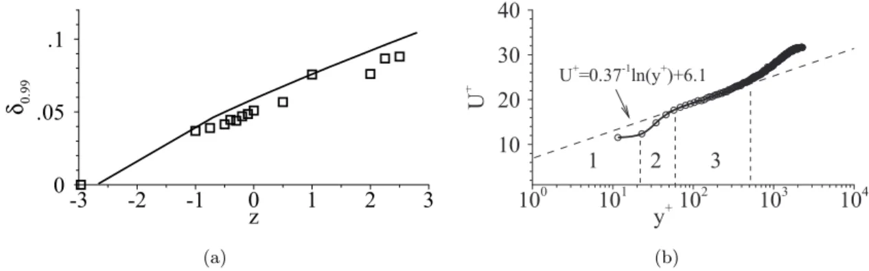
(a) c y 3 − 3y_c 09 . 2 1 1 ln 2 ≈ − + = c c c y y y y y y c yc x

x

y

c y 3 − 3y_c 09 . 2 1 1 ln 2 ≈ − + = c c c y y y y y y c yc x c y 3 − 3y_c 09 . 2 1 1 ln 2 ≈ − + = c c c y y y y y y c yc x

x

y

(b)

Figure 3.1: (a) Schematic view of the vortex pair, (b) point vortex model. The limiting stream-line of the vortex pair, also known as Kelvin oval, is shown in thick solid stream-line.

We consider a vortex pair such as the one depicted in figure 3.1. Cartesian coordinates x, y and z are used, with z in the direction of the vortex axis and x and y the transverse directions. Unitary vectors corresponding to these directions are ex, ey and ez. The vortex

pair is symmetric about the plane y = 0. At z = constant, the center of the top vortex is (xc, yc), which is the barycenter of the axial vorticity Ωz, calculated according to

xc = R y>0Ωzxdxdy Γ yc = R y>0Ωzydxdy Γ (3.1)

Stabilité des paires de tourbillons contra-rotatifs: application au tourbillon de jeu dans les turbomachines

HAL Id: pastel-00005529

https://pastel.archives-ouvertes.fr/pastel-00005529

Stabilité des paires de tourbillons contra-rotatifs:

application au tourbillon de jeu dans les turbomachines

Vincent Brion

To cite this version:

THÈSE DE DOCTORAT

DE L’ÉCOLE POLYTECHNIQUE

présentée par

Vincent Brion

pour obtenir le titre de

Docteur de l’Ecole Polytechnique

Spécialité : Mécanique

Stabilité des paires de tourbillons contra-rotatifs:

application au tourbillon de jeu dans les turbomachines

soutenue le 7 octobre 2009

devant le jury composé de :

M. P. Brancher

M. G. Casalis

M. L. Jacquin

Directeur de thèse

M. F. Leboeuf

M. T. Leweke

Rapporteur

M. M. Rossi

Rapporteur

M. P. J. Schmid

Résumé

Abstract

Remerciements

Contents

Nomenclature

1

General introduction

year of certification

thr

us

t

spe

ci

fi

c

co

ns

um

pt

ion

1.1

Tip clearance vortex

tip

leakage

vortex

rotation

(compressor)

leakage

blade

upstream

flow

casing

wall

1.2

Objectives of the thesis

1.3

Approach

1.4

Organization of the thesis

2

Review on the stability of vortices

2.1

Single vortices

2.2

Vortex pairs

2.3

Important problems of vortex dynamics

Part I

3

Numerical method

3.1

Perturbation theory