Distributed Optical Fibre Sensing System for Civil and
Geotechnical Infrastructures
Mémoire
Long Cui
Maîtrise en génie électrique - avec mémoire
Maître ès sciences (M. Sc.)
Distributed Optical Fibre Sensing System for Civil and
Geotechnical Infrastructures
Mémoire
Long Cui
Sous la direction de:
Supervisor: Sophie LaRochelle
Co-supervisor: Younès Messaddeq
Résumé
Les capteurs à fibre optique distribués (DFS) tirant parti des mécanismes de diffusion se produisant dans l’élément détecteur de fibre, à savoir la diffusion de Rayleigh, Raman et Brillouin, ont été un sujet de recherche intense au cours des trois dernières décennies. Ils offrent de nombreuses applications pratiques classées en raison des avantages inhérents, tels que la petite taille, le poids léger, la sensibilité élevée, les performances excellentes, la durabilité intrinsèque dans des environnements difficiles, l’immunité aux interférences électromagnétiques (EMI), etc.
En particulier, le DFS basé sur le processus de diffusion stimulée de Brillouin (SBS), appelé analyse temporelle optique de domaine de Brillouin (BOTDA), présente la capacité potentielle de réaliser la télédétection sur de longues distances, typiquement des dizaines de kilomètres et des centaines de kilomètres récemment. La fibre optique servant non seulement d’élément de détection, mais également de moyen de guidage de la lumière, est capable de détecter divers paramètres physiques d’intérêt, tels que la température, les contraintes, les pressions et les champs acoustiques. Ces measurandes peuvent être détectés directement ou indirectement le long de la fibre entière.
Les systèmes de pergélisol dans le Nord canadien sont fortement perturbés par les changements climatiques dus au réchauffement de la planète; le dégel du pergélisol affecte à son tour les environnements et les communautés. Afin de réaliser une surveillance en temps réel de la stabilité des infrastructures, un réseau de détection BOTDA doté d'un nouveau transducteur à fibre optique est proposé pour surveiller les modifications physiques, notamment les pressions interstitielles, la température et le déplacement dans le pergélisol. Le principal défi consiste à mesurer simultanément les pressions d’eau interstitielle positive et négative, et à faire la distinction entre ces measurandes au sein d’un même transducteur. Lors de la première tentative, un polymère d'hydrogel est utilisé pour construire le transducteur, qui peut se dilater ou se contracter du fait de l'absorption ou de la libération d'eau par le matériau afin de détecter les pressions positives et négatives dans la plage cible de -100 kPa à +100 kPa le long d'un pergélisol système. Une fibre multi-cœur (MCF) bien conçue, incorporée dans le transducteur polymère, sera développée dans le but ultime de disposer de fonctionnalités de détection simultanée de plusieurs paramètres.
Abstract
Distributed optical fibre sensors (DOFS) taking advantage of the scattering mechanisms occurring within the fibre sensing element, i.e. Rayleigh, Raman and Brillouin scattering, have been an intense research subject over the last three decades. They offer widespread practical in-filed applications due to the inherent advantages possessed, such as small size, light weight, high sensitivity, excellent performance, intrinsic durability to harsh environment, immunity to electromagnetic interference (EMI), and so on.
Particularly, the one based on stimulated Brillouin scattering (SBS) process, so-called Brillouin optical time-domain analysis (BOTDA), presents the potential capability to perform remote sensing over long distance, typically tens of kilometres and extended to hundreds of kilometres recently. Optical fibre acting as not only a sensing element but also as a light guidance medium is able to detect a variety of physical parameters of interest, such as temperature, strain, pressure and acoustic fields to name a few. These measurands can be sensed either by directly or indirectly along the whole fibre.
Permafrost systems in Northern Canada are strongly disturbed by the climate changes due to global warming; the thawing permafrost is in turn affecting the environments and communities. In order to achieve real-time surveillance of the stability of infrastructures, a BOTDA sensing network with novel fibre transducer is proposed to monitor the physical changes including positive/negative pore water pressures, temperature and displacement along permafrost environments. The main challenge is to measure simultaneously the positive and negative pore water pressures and to discriminate among those measurands within a single transducer. As an initial attempt, a hydrogel polymer is deployed to build the transducer, which can expand or shrink due to water absorption or release by the material to detect positive and negative pressures in the target range of -100 kPa to +100 kilopascal along a permafrost system. A well-designed multi-core fibre (MCF) incorporated into the polymer transducer will be developed as the ultimate goal to fulfil concurrent multi-parameter sensing functionality.
Table of contents
Résumé ... ii
Abstract ... iii
Table of contents ... iv
List of tables ... vi
List of figures ... vii
List of abbreviations ... x
List of symbols ... xiii
Acknowledgement ... xvi
Introduction ... 1
1.1 Introduction to optical fibre sensors ... 1
1.2 Single-point optical fibre sensors ... 1
1.2.1 Interferometric-based single-point sensors ... 2
1.2.2 Grating-based single-point sensors ... 8
1.3 Quasi-distributed optical fibre sensors ... 14
1.4 Fully-distributed optical fibre sensors ... 16
1.5 Permafrost system and related point sensors ... 19
1.6 Motivation and objectives ... 27
1.7 Organization of the thesis ... 28
1.8 Conclusion ... 28
2. Distributed optical fibre sensors ... 30
2.1 Introduction ... 30
2.2 Rayleigh distributed optical fibre sensors ... 32
2.3 Raman distributed optical fibre sensors... 36
2.4 Brillouin distributed optical fibre sensors ... 38
2.5 Conclusion ... 47
3. Experimental works and results ... 48
3.1 Introduction ... 48
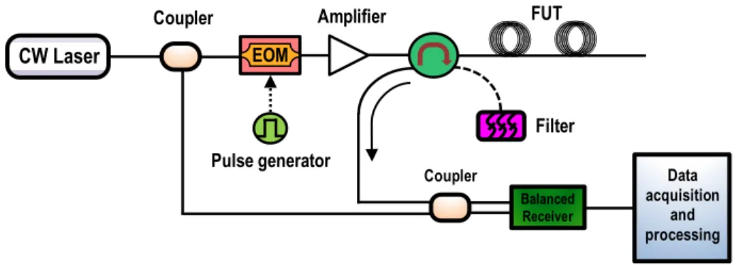
3.2 Experimental setup for BOTDA system ... 48
3.3 Experimental results and discussion ... 51
3.5 Conclusion ... 69
4. Image denoising techniques ... 70
4.1 Introduction ... 70
4.2 The proposed BM3D algorithm ... 71
4.3 Results and discussion ... 77
4.4 Conclusion ... 84
Conclusion... 85
Summary of work ... 85
Limitation of novel materials and fibre transducers ... 86
Perspectives ... 86
List of tables
1.1 Methodologies of OFSs by topology ... 1
1.2 Some specifications of the two PM-PCFs... 23
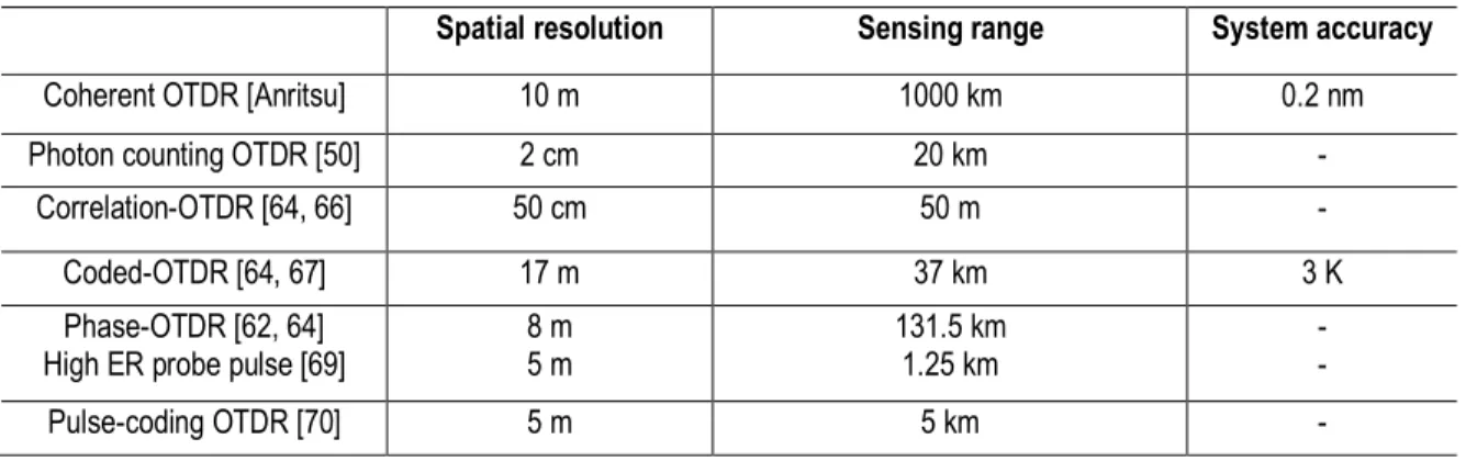
2.1 The performance parameters for various Rayleigh distributed sensing systems ... 35
2.2 Various sensing schemes in Brillouin-DOFS ... 42
2.3 The performance parameters for various Brillouin-DOFSs ... 46
3.1 Key features of the components used in our BOTDA sensing system ... 50
3.2 The parameter values for a conventional SMF used in the theoretical model... 56
3.3 The temperature measurement results along with a thermocouple... 62
4.1 The parameter values used in the proposed BM3D algorithm ... 79
4.2 The temperatures calculated from Fig. 4.4 b) ... 81
4.3 The spatial resolutions calculated from Fig. 4.5 ... 81
4.4 The temperatures calculated from Fig. 4.7 ... 83
List of figures
1.1 A schematic plot of a single-point OFS ... 2
1.2 A schematic diagram of an FPI ... 3
1.3 Configurations of an extrinsic (left) and intrinsic (right) FPI-based in-line fibre sensors ... 3
1.4 A basic configuration of an MI ... 4
1.5 Configurations of MI-OFSs using a) an optical coupler and b) a long-period grating (LPG) ... 5
1.6 A schematic representation of an SI ... 5
1.7 A schematic view of an SI-OFS ... 6
1.8 A schematic diagram of an MZI ... 7
1.9 Various schemes of in-line fibre MZIs ... 7
1.10 A schematic working explanation of an LPG in a fibre ... 8
1.11 A schematic diagram representing an FBG ... 11
1.12 A measurement setup of an FBG-based sensor with an OSA ... 13
1.13 The interrogation setup of an FBG-based sensor with filters ... 14
1.14 Quasi-distributed sensing configurations with multiplexing schemes based on a) WDM technique, b) TDM technique, c) and d) hybrid technique of WDM and TDM... 15
1.15 Various scattering processes in a standard SMF showing Rayleigh, Raman, and Brillouin shifts with Stoke and anti-Stokes signals ... 17
1.16 Rayleigh scattering due to microscopic-scale variations in RI ... 17
1.17 Energy diagram of a) Stokes and b) anti-Stokes processes ... 18
1.18 Permafrost distribution across Northern Canada ... 19
1.19 A permafrost system and related occurrence during its thawing ... 20
1.20 Examples of damaged infrastructures ... 20
1.21 An active layer in a soil environment showing the linear positive/negative PWPs depending on the water depth from the water table ... 21
1.22 A structure of the vibrating wire piezometer... 22
1.23 A structure of the electrical resistance piezometer ... 23
1.24 The PM-PCFs and transducers for in-line fibre interferometric point sensor measuring PWPs ... 23
1.25 The design of an FBG sensor for measuring PWP ... 25
1.26 Thermal profile of a permafrost environment ... 26
1.27 On-site pictures of a permafrost environment in Umiujaq area ... 27
2.1 A schematic diagram of an OTDR system and its retroreflected optical signal detected at the photodetector (PD) ... 30
2.2 A schematic diagram of an OFDR system ... 31
2.4 A schematic diagram of a coded-OTDR ... 34
2.5 A schematic diagram of an intensity-measuring phase-OTDR ... 35
2.6 A schematic diagram of a typical RDTS system to measure the normalised Raman ratio ... 37
2.7 Double-ended RDTS system ... 37
2.8 A schematic diagram representing the SBS process in a fibre ... 39
2.9 The SBS phenomenon occurring in a pump-probe configuration... 39
2.10 The circulating SBS process... 40
2.11 A typical setup of a BOTDR system ... 42
2.12 A basic experimental BOTDA system ... 43
2.13 An example of 3D-BGS as a function of the fibre length and detuning frequency... 44
3.1 The experimental setup for BOTDA system showing a) the picture and b) the schematic diagram ... 49
3.2 A train of created pump pulse signals with a zoom to show the 20 ns pulse width ... 52
3.3 An example of generated double-sideband CW probe signal ... 53
3.4 The reflection spectrum of the narrowband FBG filter ... 54
3.5 Some examples of measured Brillouin gain signals with different fibre lengths a) L=2 km, b) L=10 km, and c) L=20 km ... 55
3.6 The measured a) 3D- and b) 2D-BGS along a 2 km fibre length of Corning SMF-28 fibre ... 57
3.7 The measured Brillouin gain signals at a) the near-end and b) the far-end of the FUT along with the Lorentzian fitted shape ... 58
3.8 The setup for measuring temperature/strain responses of the FUT ... 59
3.9 Brillouin gain signals with temperature change at different frequency offsets a) fD=10.860 GHz, and b) fD=10.896 GHz ... 60
3.10 Brillouin gain signals with an applied axial strain at different frequency offsets a) fD=10.860 GHz, and b) fD=10.896 GHz ... 60
3.11 The variations of BFS against the changes of a) temperature and b) axial strain ... 61
3.12 The variations of BFS of the system by repeating the measurement of BGS at different times ... 62
3.13 The working principle of transducer in the active layer of a permafrost system ... 63
3.14 The built water tank enabling variable pressures according to the height of water column, H ... 64
3.15 The fibre transducer made from a porous plastic material (PE) with optical fibre wrapped around the cylinder ... 64
3.16 The responses of the fibre transducers from different PWPs ... 65
3.17 The solid PVA cylinder with diameter of 10 cm ... 66
3.18 The first design of transducer fabricated from PAR ... 66
3.19 The second trial of transducer design fabricated from PAR... 67
3.20 The measurement result in water tank from PAR transducers... 67
3.21 An FBG sensor attached to a transducer made by PAR ... 68
4.1 The raw data of a) 3D-BGD and b) 2D-BGS with the average of 16 and the sampling rate of 250 Msa/s from real-time oscilloscope (RTO) ... 78 4.2 The 3D-BGS with sampling rate of 250 Msa/s showing a) raw data and b) denoised by BM3D with SNR improvement of 30dB ... 79 4.3 The 2D-BGS with sampling rate of 250 Msa/s showing a) raw data and b) denoised by BM3D with SNR improvement of 30dB ... 80 4.4 Temperature distribution along the FUT with different SNR improvements a) around 2 km fibre section and b) around the heated fibre section... 81 4.5 The estimate of spatial resolution with sampling rate of 250 Msa/s for various SNR improvements ... 82 4.6 The 2D-BGS with sampling rate of 1000 Msa/s showing a) raw data and b) denoised by BM3D with SNR improvement of 30dB ... 82 4.7 Temperature distribution of the heated fibre section with different SNR improvements ... 83 4.8 The estimate of spatial resolution with sampling rate of 1000 Msa/s for various SNR improvements ... 84
List of abbreviations
AWGN additive white Gaussian noise
BFS Brillouin frequency shift
BGS Brillouin gain spectrum
BM3D block-matching and 3D filtering
BOCDA Brillouin optical correlation-domain analysis BOCDR Brillouin optical correlation-domain reflectometry BOFDA Brillouin optical frequency-domain analysis BOFDR Brillouin optical frequency-domain reflectometry BOTDA Brillouin optical time-domain analysis
BOTDR Brillouin optical time-domain reflectometry
BS beam splitter
CH4 methane
CO2 carbon dioxide
CW continuous wave
DAS distributed acoustic sensing
DOFS distributed optical fibre sensor
DPP-BOTDA differential pulse-width pair BOTDA
DVS distributed vibration sensing
EDFA erbium-doped fibre amplifier
EMI electromagnetic interference
EOM electro-optic modulator
ER extinction ratio
FBG fibre Bragg grating
FDM frequency-division multiplexing
FFT fast Fourier transform
FMF few-mode fibre
FOSS fibre optic sensing system
FPI Fabry-Pérot interferometer
FSR free spectral range
FUT fibre under test
FWHM full width at half-maximum
HF-PCF high-birefringence PCF
IFFT inverse fast Fourier transform
LO local oscillator
LPG long-period grating
MCF multicore fibre
MI Michelson interferometer
MMF multi-mode fibre
MOF microstructured optical fibre
MZI Mach-Zehnder interferometer
NLM non-local means
OBR optical backscatter reflectometry
OFDR optical frequency-domain reflectometry
OFS optical fibre sensor
OPD optical path difference
OSA optical spectrum analyser
OTDR optical time-domain reflectometry
OTF optical tunable filter
PAR polyacrylate resin
PC polarization controller
PCF photonic crystal fibre
PD photodetector
PMF polarization-maintaining fibre
PWP pore water pressure
PPP-BOTDA pulse pre-pump BOTDA
PE polyethylene
PP polypropylene
PS polarization scrambler
PTFE polytetrafluoroethylene
PVA polyvinyl alcohol
PVDF polyvinylidene fluoride
RDTS Raman distributed temperature sensing
RI refractive index
RTO real-time oscilloscope
SBS stimulated Brillouin scattering
SDM space-division multiplexing
SHM structural health monitoring
SI Sagnac interferometer
SNR signal-to-noise ratio
SOA semiconductor optical amplifier
SOP states of polarization
SpBS spontaneous Brillouin scattering
SPM self-phase modulation
SPN sampling point number
SpRS spontaneous Raman scattering
SRS stimulated Raman scattering
TDM time-division multiplexing
TLS tunable laser source
UV ultraviolet
WD wavelet denoising
List of symbols
𝑨𝒆𝒇𝒇 effective mode area of an optical fibre
𝑩 birefringence of a PMF
𝒄 speed of light in vacuum
𝑪𝜺 strain coefficient against the variation of BFS 𝑪𝑻 temperature coefficient against the variation of BFS 𝒅 etching depth of the phase-mask for writing an FBG
𝑬 Young’s modulus of a material
𝑬𝑩𝑺 field of the backscattered signal in C-OTDR
𝑬𝑳𝑶 field of local oscillator in C-OTDR
𝑬𝒕𝒐𝒕 field at the detection end, where the backscattered signal is interfered with the reference signal through balanced detection in C-OTDR
𝒇𝒃 specific frequency in the spectrum of the light pulse in OFDR
𝒇𝑫 detuning frequency in BOTDA
𝒇𝒎 modulation frequency in BOCDA or BOCDR
𝒇𝒎𝒂𝒙, 𝒇𝒎𝒊𝒏 maximum or minimum modulation frequencies in BOFDA or BOFDR
𝒈𝑩 Brillouin gain coefficient
𝒉 Planck constant
𝑯 height of water column in the built water tank for BOTDA 𝑰𝑴 intensity of backscattered signal with static condition in Φ-OTDR
𝑰𝑴𝒑 intensity of backscattered signal with perturbed in Φ-OTDR
𝒊𝒑𝒉𝒐𝒕 photodetector current in C-OTDR
𝑲𝒂𝒔, 𝑲𝒔 coefficients to the cross-sections of anti-Stokes and Stokes
𝒌𝑩 Boltzmann constant
𝒌𝒎 coupling coefficient for mth-order cladding mode in an LPG
𝒌B coefficient of birefringence-pressure in PM-PCF SI-based PWP sensor
𝑳𝒆𝒇𝒇 effective fibre length
𝑳𝒎𝒂𝒙 measuring range in BOFDA or BOFDR
𝒏 refractive index
𝒏𝒆𝒇𝒇 effective refractive index of the fibre core
𝒏𝒈,𝒆𝒇𝒇 effective group index of the guided mode in an fibre
𝑵𝑴 maximum number of similar blocks to form a group in BM3D
𝑵𝒔 search window size in BM3D
𝒑𝟏𝟐 photo-elastic constant
𝑷𝒂𝒔(𝒛) power of the anti-Stokes Raman backscattered signal 𝑷𝒔(𝒛) power of the Stokes Raman backscattered signal
𝑷𝒑 pump power in Brillouin-based DOFS
𝑷𝒔 probe or Stokes power in Brillouin-based DOFS
𝑹𝒅 responsivity of a PD
𝑹(𝑻, 𝒛) power ration of anti-Stokes and Stokes Raman backscattered signals 𝑹K(𝑻, 𝒛) normalised Raman ratio in RTDS
𝒓𝒖,𝒗 reflectivity at position u and v in Φ-OTDR
𝒕 time
𝑻 temperature
𝑻𝒎 transmission of the resonant peaks in an LPG
𝑻𝒑 pulse width of the pump signal in BOTDA
𝑻𝒓 sweep duration of the light pulse in OFDR
𝑻𝒓𝒆𝒇 temperature to the end of the reference coil in RTDS
𝒖 pore water pressure
VA acoustic velocity
𝒗𝒈 group velocity
𝒘 amount of deflection of a plate due to applied pressure in an FBG-based PWP sensor
𝒛 fibre distance
𝒛𝒑 perturbed location in Φ-OTDR
𝒛𝒓𝒆𝒇 distance to the end of the reference coil in RTDS
𝜶 attenuation loss of a fibre
𝜶𝒎 thermal expansion of a material
𝜶𝒂𝒔, 𝜶𝒔 backscattered losses at the anti-Stokes or Stokes frequencies in RDTS
𝜷 propagation constant
𝜸𝒘 unit weight of water
∆𝑪𝜺 deviation of strain coefficient in BOTDA ∆𝑪𝑻 deviation of temperature coefficient in BOTDA ∆𝒇 frequency sweep range of the light pulse in OFDR
∆𝒇𝒎 step of modulation frequency in BOFDA or BOFDR
∆𝑰 intensity change at backscattered signal in Φ-OTDR
∆𝑳 axial extension of a fibre
∆𝑷 change of surrounding pressure in PM-PCF SI-based PWP sensor
∆𝑻 temperature difference
∆𝝀 wavelength shift from the pressure-dependent birefringence in PM-PCF SI-based PWP sensor
∆𝝂 Raman frequency shift
∆𝝂𝑩 FWHM of a Brillouin backscattered signal
∆𝒛 spatial resolution of a distributed sensing system 𝜹 relative phase difference of an interferometer sensor
𝜹𝟎 intrinsic birefringence phase shift in PM-PCF SI-based PWP sensor
𝜹𝒑 pressure-induced birefringence phase shift in PM-PCF SI-based PWP sensor
𝜺 applied axial strain
𝜺𝒓 relative strain
𝜼 thermo-optic coefficient of a material
𝜽𝒑 phase change due to perturbation in Φ-OTDR
𝝀 wavelength of an incident light
𝝀𝑩 Bragg wavelength of an FBG
𝝀𝒎 resonant wavelength corresponding to the coupling to the mth-order cladding
mode in an LPG
𝝀𝒑 wavelength of pump wave in Brillouin-based DOFS
𝝀𝑼𝑽 wavelength of UV light used for writing an FBG
𝚲 grating pitch of an FBG
𝚲𝒑𝒎 period of etched grooves in a phase-mask for writing an FBG
𝝊 Poisson’s ratio of a material
𝝂𝑩 Brillouin frequency shift
𝝆 material density
𝝆𝒆 photo-elastic coefficient
𝝉 pulse width of the light source in distributed sensing system 𝝓𝒊 total phase change of light at the 𝑖th scattering element in Φ-OTDR 𝝓𝒖,𝒗 corresponding phases at position 𝑢 and 𝑣 in Φ-OTDR
Acknowledgement
I would like to appreciate all those who have contributed in a way to my research project and as well as those who have made my life here very pleasant and fruitful.
First and foremost, I’m sincerely grateful to my supervisors, Sophie LaRochelle and Younès Messaddeq, for giving me the opportunity to perform a research project in the field of distributed optical fibre sensors. Their constructive guidance and supportive comments throughout the study have helped to shape the way in which this material is presented. I also would like to express my gratitude to the Sentinelle Nord for the financial support of the project.
Special thanks to the postdoctoral researchers, Ruohui Wang, Amir Tork, Xun Guan and Junho Chang for their help to better understand those devices and equipment involved throughout the course of implementation for the distributed sensing system. Their useful suggestions through discussion and advice when needed have led me to tackle effectively with the problems I have faced while carrying out the experimental system. Many thanks to the lab technician, Simon Levasseur, for his assistance to build the system of water tank realising different water pressures in accordance with water column.
Thanks also to my colleagues, Omid Jafari, Alessandro Corsi, Antoine Gervais, Gabriel Lachance, Charles Matte-Breton, Rezan Homay, Ali Riaz, Joy Roy, Ismail Amar, and Douglas Franco, for sharing information and knowledge not only in research but also in daily life.
Last but not least, I’m deeply indebted to my family and this could not have been done without their continuous support and constant love.
Introduction
1.1 Introduction to optical fibre sensors
In company with the revolutionary progress in optical telecommunications, led by the combination of innovative invention of optical fibres and improvements in optoelectronic components, the field of optical fibre sensing technology has been grown tremendously along with it through intense researches in laboratory fuelled by practical in-field applications.
Optical fibre sensors (OFSs) are devices that transport the modulated light in response to the surrounding physical parameters. The light modulated in wavelength/frequency, intensity, polarization or in phase, is interpreted with an interrogator to estimate the change of these properties in response to temperature or strain. The transducer, the optical fibre and the interrogator make the entire fibre optic sensing system (FOSS), which occupies a large section of high precision sensor market share nowadays.
The methodologies of FOSS can be classified into three main domains according to their topologies, i.e. single-point, quasi-distributed (multi-point) and fully-distributed sensing strategies, which is listed in Table 1.1 and will be shortly described in the following sections.
Single-point Quasi-distributed Fully-distributed
Sensor types § Interferometric sensors § Grating-based sensors - LPGs - FBGs § Time-division multiplexing (TDM) § Frequency-division multiplexing (FDM) § Spatial-division multiplexing (SDM) § Rayleigh scattering § Raman scattering § Brillouin scattering
1.2 Single-point optical fibre sensors
As the name refers, a single-point sensor is useful to detect a parameter of interest at a predefined location. As schematically illustrated in Fig. 1.1, a single-point OFS is preferred when a specific location is to be monitored, benefiting from their features such as small size, simple, handiness, and so on. Usually, the sensing unit/element
or the transducer is at the fibre end tip working as a probe to receive the modulated signal by an external parameter change and guide it to the detector. Then, the modulated signal can be translated into the parameter change. Several optical thermometers and strain gauges belong to this sensing category and have been some of the first applications of OFS. In addition, the field of chemical-, medical- and bio-sensors are increasingly investigated and are a leading direction of research for new applications of OFS.
Two of the most widely commercially available and well-known single-point sensor methodologies are discussed in the following sections.
1.2.1 Interferometric-based single-point sensors
Interference is a basic optical phenomenon taking place during the interaction between light waves, in which the optical field of two given waves overlap. This can be deployed in a sensing scheme by constructing different types of optical interferometers. An interference is formed between two light beams that propagate with different optical path lengths within a single fibre or two. One of the optical paths is arranged to be easily affected by external perturbations such that the interference signal is modulated in wavelength, frequency, intensity, phase, polarization, and so on. Therefore, the measurand can be quantitatively determined by measuring the change in this spectral information. Miniaturizing them into a micro/nano-scale size is an emerging trend for pressure or temperature sensing in medical treatment. In order to realize such reduced dimension, several in-line structures have been explored as promising candidates due to their peculiar properties such as high coupling efficiency, simple alignment and excellent stability. Fibre-optic interferometers can be divided into four well-known representatives: i.e. Fabry-Pérot, Michelson, Sagnac and Mach-Zehnder. A short description of their working principles, compact building blocks and specific applications is followed.
Firstly, Fabry-Pérot interferometers (FPIs) or etalon are generally constructed with two parallel and partially reflecting surfaces or mirrors separated by a certain distance [1]. The interference takes place by multiple
Cladding Core Cladding Measurand Light modulated Sensing unit
superpositions from both reflected and transmitted beams at the parallel surfaces, which is schematically shown in Fig. 1.2.
The structures of FPIs within an optical fibre can be realized extrinsically or intrinsically depending on the location of a cavity, as illustrated in the following Fig. 1.3 [2, 3].
In extrinsic in-line fibre FPIs shown in the left of Fig. 1.3, an external cavity is generally formed by air or polymers with supporting structures for temperature-insensitive strain [4], pressure [5], displacement [6], refractive index (RI) [7], molecule detection or gas sensing [8]. The fabrication is relatively easy, simple and cost-effective but it possesses low coupling efficiency, alignment is difficult and it presents packaging issues. On the other hand, the local cavity of an intrinsic in-line fibre FPI can be shaped using two reflectors fabricated by means of micro-machining [9], fibre Bragg gratins (FBGs) [10], chemical etching [11] or thin-film deposition [12]. Clearly, these techniques are costly and risky. However, it provides high-intensity optical signal and, in turn, better signal demodulation since the light signal is propagating within the fibre itself all the time. Along with the development and improvement of specialty optical fibres and fibre-based devices, novel operating configurations based on a variety of microstructured optical fibres (MOFs) or photonic crystal fibres (PCFs) have been proposed [13]. Furthermore, simultaneous multi-parameter measurement could be accomplished through combining FPI and grating techniques [14].
The spectral information, reflection or transmission of an in-line fibre FPI sensor, can be explained as the wavelength dependent intensity modulation of an incident light, which is due to the optical phase difference
Mirror 2 Mirror 1 Incident Reflected Transmitted Cavity
Figure 1.2 A schematic diagram of an FPI
Mirror #1 Mirror #2
L L
Air, Polymer, etc.
between two reflected or transmitted waves at the two reflecting mirrors. The relative phase difference induced by the optical path difference (OPD) between two reflected beams is simply given as,
𝛿ghi=2𝜋
𝜆 (𝑛2𝐿) (1.1) where 𝜆 is the wavelength of the incident beam, 𝑛 is the RI of the cavity, and 𝐿 is the physical length of the cavity [15]. The maximum and minimum peaks of the modulated spectrum appear when the beams are in-phase and out-of-phase, respectively, at a particular wavelength. When an external perturbation is introduced, the phase difference is varied as the OPD (both refractive index and physical length) is modified, which is the base of working principle for FPI-based in-line fibre sensors. Therefore, a quantitative measurand can be estimated by calculating the wavelength shift in the spectrum. The free spectral range (FSR), the spacing in optical wavelengths between two successive maxima or minima in the interference pattern, is also affected by the OPD change. The variation in FSR gives a trade-off between the dynamic range and resolution of a sensor [16]. For instance, shorter OPD presents wider FSR, which certainly provides larger dynamic range; in the meanwhile, it gives poor resolution due to blunt peak signals. Consequently, there is a compromise between these two performance indicators that must be optimised according to the specific application targeted.
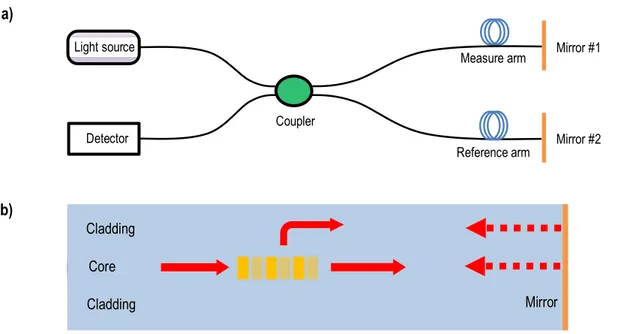
Secondly, Michelson interferometers (MIs) are established through a beam splitter to separate an incident light into two arms and using mirrors to reflect them back to the splitter and combine them to generate an interference pattern by superposition, which is shown in Fig. 1.4 [1]. Similarly, MI-based OFSs (MI-OFSs) are built in several ways by using reflecting mirrors as schematically displayed in Fig. 1.5 a) and b).
Beam splitter
Light source Mirror #1
Mirror #2
Detector
In Fig. 1.5 a), the incident beam is split into two arms, reference and measure (or sensing) arms, via an optical directional coupler and reflected back to the detector through the mirror in each arm. In addition, a compact in-line fibre structure as shown in Fig. 1.5 b) can be realized by long-period grating (LPG) techniques [17] so that it causes cladding modes coupled from core modes and then back-reflected by a mirror manufactured with a metallic film at the end tip of a fibre. Intense studies have been explored with novel PCFs for sensing various measurands [18]. They are simple, handy and favourable to fulfil multi-point sensing system by connecting them in parallel through multiplexing techniques.
The working principle of these sensors is similar to that explained previously, which is based on the phase variation of the interference beam due to the OPD change in sensing arm and this results in the wavelength or frequency shift according to the measurand change.
Mirror #1 Measure arm Light source Mirror #2 Reference arm Coupler Detector Cladding Core Cladding Mirror
Figure 1.5 Configurations of MI-OFSs using a) an optical coupler and b) a long-period grating (LPG)
Light source
Detector
Figure 1.6 A schematic representation of an SI a)
Thirdly, Sagnac interferometers (SIs) are arranged by a rotating loop in which the incident beam is divided in two and propagates in counter directions, as shown in Fig. 1.6 [1]. In case of optical fibres, it is very simple to assemble to form an SI as illustrated in Fig. 1.7 by means of coupler and polarization controller (PC) to get the two counter-propagating beams to have different polarization states; one is in slow axis and the other is in the direction of fast axis.
Unlike the other interferometers, the OPD in an SI-OFS is determined by the different polarization-dependent propagating speed of the mode guided along the closed path. The phase of the interference is given by,
𝛿si=2𝜋
𝜆 (𝐵𝐿), 𝐵 = u𝑛v− 𝑛xu (1.2) where 𝐵 is the birefringent coefficient of the sensing fibre, 𝐿 is the length of the sensing fibre, 𝑛v and 𝑛x are the effective indices of the fast and slow modes, respectively [19]. As indicated from the Eq. 1.2, higher birefringence refers to better sensitivity of phase modulated. Thus, high-birefringence PCFs (HB-PCFs) or polarization-maintaining fibres (PMFs) are deployed as sensing fibres for measuring temperature, pressure, torsion, and so on [19, 20]. One of the beneficial aspects of SI-OFSs is the capability of simultaneous multi-parameter sensing via a hybrid of Sagnac and Mach-Zehnder sensor using PMF and LPG techniques [21] or through a novel PCF [22].
Light source Detector
PC
Sensing fibre Coupler
Splice
Fourthly, MZIs can be established in optical fibres using diverse configurations (LPG-pair, core-mismatch, PCF or MMF, tapering, etc.) as depicted in Fig. 1.9, which makes it very flexible for sensing many physical changes [23].
Here, the modulated phases are determined by the OPDs, due to modal effective indices and dispersion of core and cladding modes, which is given as,
𝛿yzi =2𝜋 𝜆 {∆𝑛|vv} 𝐿~ (1.3) Detector Light source Detector BS1 BS2
Figure 1.8 A schematic diagram of an MZI
LPG pair
Core offset
PCF or MMF
where ∆𝑛|vv} is the effective RI difference between the core and 𝑚th cladding mode and 𝐿 is the propagation
length of the modes. By designing appropriate building blocks through adjusting the RI difference, a compact-size sensing element could be realized for specific application fields. In the same way, it could also provide the capability to measure multi-measurand simultaneously by using an in-fibre grating approach into MZIs [24].
1.2.2 Grating-based single-point sensors
Another popular branch of extensively and explosively studied point sensors is based on grating techniques, namely long-period gratings (LPGs) and fibre Bragg gratings (FBGs). The periodic perturbation of RI in an optical fibre core is referred to as a fibre grating. The photosensitive core material is modulated while exposed to a light with specific wavelength and intensity. This kind of change in RI essentially leads to a spectral modulation in transmission or in reflection modes through the coupling from propagating core modes to cladding modes or through the coupling between forward and backward propagating core modes, respectively, depending on the grating period, i.e. the modulation period of the RI. The former is the case of LPGs and the latter is the case for FBGs.
Firstly, the LPGs in optical fibres are fabricated by introducing a periodic modification of RI in the fibre core through a number of approaches either by mechanical ways or by laser irradiation techniques [25]. The pitch or the period of RI modulation is in the order of 100 µm and even up to 1 mm. A regular transmission spectrum of an LPG possesses several attenuation dips at distinct resonant wavelengths, each corresponding to the coupling between the guided core mode and a particular cladding mode, which is the case schematically illustrated in the following Fig. 1.10.
The central resonant wavelengths at the transmission spectrum are affected by the composition of the fibre, the grating pitch, the length of an LPG, and the local environmental changes such as temperature, surrounding RI, strain, and so on. With an inscribed LPG in a specific fibre, any perturbations in those parameters can modify
Cladding Core Cladding
Input spectrum LPG Transmitted spectrum
the grating pitch and/or the differential RI of the core and cladding modes. This alters the phase-matching conditions for the coupling to the cladding modes, which results in the shift of central resonant dips. This forms the principle of operation mechanism based on LPG sensors and will be explained analytically in the following. The phase-matching condition in an LPG is expressed as,
𝛽‚ƒ− 𝛽‚„} = Δ𝛽 =2𝜋
Λ (1.4) where 𝛽‚ƒ and 𝛽‚„} are propagation constants of the core mode and the 𝑚th-order co-propagating cladding
mode, respectively, and Λ is the grating pitch. From it, the condition of resonant wavelength is derived as,
𝜆} = ˆ𝑛|vv‚ƒ − 𝑛|vv‚„,}‰Λ, 𝛿𝑛|vv = 𝑛|vv‚ƒ − 𝑛|vv‚„,} (1.5)
where 𝜆} is the resonant wavelength corresponding to the coupling to the 𝑚th-order cladding mode, 𝑛
|vv ‚ƒ and
𝑛|vv‚„,} are the effective RI of the core mode and the 𝑚th-order cladding mode, and their difference is 𝛿𝑛
|vv.
The transmission of the resonant peaks is given by,
𝑇}= 1 − 𝑠𝑖𝑛•(𝑘}𝐿) (1.6)
where 𝑘} is the coupling coefficient for 𝑚th-order cladding mode and 𝐿 is the length of grating. The coupling
strength depends on the overlap integral between core and cladding modes, i.e. the modes having similar electric field profiles and as well by the amplitude of the periodic modulation of the mode propagation constants. Since it is sensitive to external perturbations, this leads to both amplitude change and wavelength shift of the resonant dips in the transmission spectrum [26].
As indicated in Eq. 1.5, the temperature response of an LPG sensor results from the changes of differential effective index of core/cladding modes and the changes of grating pitch due to thermo-optic effects. By taking the temperature derivative of Eq. 1.5, the sensitivity is expressed as,
𝑑𝜆} 𝑑𝑇 = 𝑑𝜆} 𝑑(𝛿𝑛|vv)‘ 𝑑𝑛|vv‚ƒ 𝑑𝑇 − 𝑑𝑛|vv‚„,} 𝑑𝑇 ’ + Λ 𝑑𝜆} 𝑑𝛬 1 𝐿 𝑑𝐿 𝑑𝑇 (1.7)
Clearly, the shift in resonant wavelength is influenced by the material contribution (the first term on the right-hand side of Eq. 1.7), i.e. the fibre composition and the order of coupled cladding mode, and the waveguide contribution (the second term), i.e. the grating pitch. At a specific wavelength, Eq. 1.5 tells that the coupling to higher-order (lower-order) cladding modes requires shorter (longer) grating pitch and this leads to negligible
(dominant) material effect; in addition, the wavelength term 𝑑𝜆}⁄𝑑𝛬 becomes negative in the case of coupling to higher-order cladding modes, while for the lower-order modes this has positive values for conventional germanosilicate fibres [28]. Hence, the desired sensing capabilities could be realised through adjusting the grating pitch for specific applications.
The strain sensitivity of an LPG sensor arises from the physical changes of fibre length, grating pitch and the difference of effective index between core/cladding due to elasto-optic effect. In much similar way to the case of temperature, the strain response can be obtained via differentiating Eq. 1.5 with respect to axial strain, which is expressed as, 𝑑𝜆} 𝑑𝜀 = 𝑑𝜆} 𝑑(𝛿𝑛|vv)‘ 𝑑𝑛|vv‚ƒ 𝑑𝜀 − 𝑑𝑛|vv‚„,} 𝑑𝜀 ’ + Λ 𝑑𝜆} 𝑑Λ (1.8)
Like previously, the strain sensitivity is also affected by the material and waveguide contributions, respectively, from the first and second term on the right-hand side of Eq. 1.8. The material effects come from the strain-optic effect (change in RI) and Poisson’s effect (change in the dimension of a fibre), while waveguide effect comes from the term 𝑑𝜆}⁄𝑑𝛬, the slope of dispersion. For longer grating pitch in standard optical fibres, the material contribution is negative, whereas the waveguide effect is positive, i.e. 𝑑𝜆}⁄𝑑𝛬> 0 [28]. Depending on the
magnitude of these two effects, the sign of strain sensitivity will be determined whether the attenuation peaks shift to longer or shorter wavelengths. The total shift of the resonant wavelength for a certain value of an axial strain is a function of the grating pitch and the order of cladding mode involved in coupling. Therefore, by properly selecting these two variables, it is attainable for the material and waveguide effects to cancel each other completely with the same magnitude but with opposite sign, which can offer strain-insensitive resonance peaks. Overall, a novel design of an LPG with a proper grating pitch could offer the solution of cross-sensitivity issue by decoupling of the temperature and strain responses, and provide simultaneous multi-parameter sensing capability as well. Characteristics based on LPG sensors such as temperature-insensitive or strain-insensitive and positive/negative responses have a large number of specific applications. Among them, the relatively high RI sensitivity to surrounding environment has been demonstrated to be a great potential for a variety of chemical [29] and biosensor applications in monitoring or detecting viruses, bacteria, toluene, air quality, and so on [30-33]. However, their multiple resonance bands and broad transmission spectra (typically tens of nanometers) limit the measurement accuracy and restrict the multiplexing capabilities employed in multi-point sensors.
The FBG-based fibre sensors have been the most successful OFS and they occupy the largest portion of the fibre market nowadays. The FBGs are realized via the periodic RI modulation in the fibre core, but the grating pitch is in the order of few hundreds of nanometers or less. Usually, they are inscribed into the photosensitive
fibres by phase-mask techniques inducing interference fringe pattern using ultraviolet (UV) or femtosecond lasers. The grating pitch is defined by the period of etched grooves in a phase-mask, which is given as,
Λ›=1
2 ΛB} (1.9) In order to achieve the minimum zeroth order of diffraction, the etching depth, 𝑑, should be adjusted to,
𝑑 =1
2 λžŸ (1.10) where λžŸ is the wavelength of UV light used. So, a different phase-mask is required for each laser writing at a
different wavelength [26]. Using this techniques, few interesting grating structures like chirped or tilted FBGs are realized for unusual properties and applications.
As for FBG, the Bragg wavelength is determined by the phase matching condition,
𝛽‚ƒ( )+ 𝛽‚ƒ(¡)=2𝜋
Λ (1.11) where (+) sign occur rather than (−) because the two core modes are counter-propagating. Therefore, only the light whose wavelength obeys this law can be reflected while the remainder is transmitted without any loss, as shown schematically in Fig. 1.11.
The back-reflected constructive interference wave possesses the peak power at a centre wavelength, so-called Bragg wavelength which is defined by the grating design. From Eq. 1.11, the Bragg wavelength can be obtained and given as,
𝜆¢ = 2 ∙ 𝑛|vv∙ 𝛬 (1.12)
where 𝑛|vv is the effective index of the core and Λ is the grating pitch. Cladding Core Cladding Input spectrum FBG Transmitted Reflected
Likewise LPG-based sensors, a variation in the axial strain or in temperature will displace the Bragg wavelength. A change in strain can increase Λ and can change the 𝑛|vv as well by photo-elastic effect. Equally, a variation
in temperature can affect both values, respectively, by thermal dilation and thermo-optic effect. Therefore, other parameters including pressure, vibration, displacement and etc. can also be estimated through the shift in Bragg wavelength with novel fibre transducers with smart designs.
In order to achieve the temperature sensitivity of an FBG sensor, the partial derivative of Eq. 1.12 with respect to temperature should be applied and it is given by [34],
∆𝜆¢ 𝜆¢ = 1 Λ 𝜕Λ 𝜕T∆𝑇 + 1 𝑛|vv 𝜕𝑛|vv 𝜕T ∆𝑇 (1.13)
On the right-hand side of Eq. 1.13, the first term is referred to as the thermal expansion (𝛼) of a material and the second term is considered as the thermo-optic effect (𝜂) of a material. Then, Eq. 1.13 becomes as,
∆𝜆¢
𝜆¢ = (𝛼 + 𝜂)∆𝑇 (1.14) In much the same way, the strain sensitivity is expressed as,
∆𝜆¢ 𝜆¢ = 1 Λ 𝜕Λ 𝜕L∆𝐿 + 1 𝑛|vv 𝜕𝑛|vv 𝜕L ∆𝐿 (1.15)
The first term on the right-hand side is the strain due to fibre elongation. If the extension is ∆𝐿 then relative strain is defined as 𝜀©= ∆𝐿/𝐿. Since the deformation of an FBG is within the fibre itself the value 𝜕Λ/𝜕L = 1. The
second term is due to the photo-elastic effect (𝜌|), which is the change of effective index with respect to the applied strain. In optical fibres, this value is negative because the RI decreases as the material density reduces as the fibre elongates. Again, the strain sensitivity can be stated as,
∆𝜆¢
𝜆¢ = (1 − 𝜌|)𝜀© (1.16) Hence, the total change is the sum of the temperature and strain sensitivities, which is represented as,
∆𝜆¢
𝜆¢ = (𝛼 + 𝜂)∆𝑇 + (1 − 𝜌|)𝜀© (1.17) For conventional germanium-doped silica fibres, the values of temperature and strain sensitivities at the range of 1550 nm are approximately estimated as,
∆𝜆¢
∆𝑇 ≈ 10 − 15 pm/℃, ∆𝜆¢
∆𝜀 ≈ 1 − 1.5 pm/µε (1.18) Of course, these values are varied according to different material compositions.
In common with other fibre sensors, the main challenge is how to discriminate the cross-sensitivity between the temperature and strain effects and to reveal the change of each parameter, ∆𝑇 and ∆𝜀. In order to overcome this issue, many effective methods have been explored for the last few decades. One of them is using a pair of FBGs experiencing same temperature sensitivity, while the other one is protected from strain change [35]. Another familiar approach is based on FBGs having large difference is their Bragg wavelengths, which results in dissimilar sensitivities to the same parameter change [36]. Besides, solutions with specialty fibres [37], with the help of nonlinear effect (Brillouin scattering) [38], or with different coating materials (acrylate or polyimide) [39] have been investigated.
The other main challenge is the interrogation techniques to detect the displacement of back-reflected Bragg wavelength as a function of measurand changes. The simplest and straightforward way is to use an optical spectrum analyser (OSA) to directly measure the reflection spectrum. In addition, the conversion from wavelength variations into optical power intensities is also applied to determine the shift of Bragg wavelength, which is very simple in measurement configuration as shown in Fig. 1.12.
However, detecting the back-reflected signals from an OSA is limited by the resolution so that it can restrict the measurement accuracy. In order to overcome this limitation, other demodulation techniques with narrowband filters, FP tunable filter or FBG filters, are applied to the measurement system, which is shown in Fig. 1.13.
FBGs Light source
Circulator
OSA
In case of FP filter, the transmission mode is applied, while for the FBG filter it is used as a dichroic mirror (reflection mode). The convolution function of back-reflected FBG sensor and the spectral response of the filter represents the power to the photodetector (PD) as a function of wavelength shift.
Having demonstrated outstanding features, i.e. small size, simple configuration, EMI-free, passive nature, and so on, FBG-based sensors have become the leading product in sensor market with in-field applications in harsh environments with high temperature, high pressure or high nuclear radiation [40] and as well in structural health monitoring (SHM) including buildings, bridges, dams, tunnels, concretes, and so on. These sensors are the mainstream in the market today.
1.3 Quasi-distributed optical fibre sensors
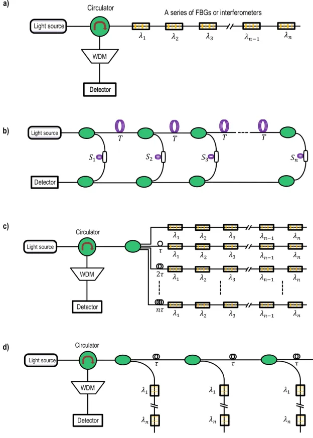
Quasi-distributed OFSs, also known as multi-point sensors, rely on multiplexing techniques to share a common light source and detection system. The entire measurement system is established by assembling those interferometric- and grating-based point sensors in series or in parallel through the multiplexing schemes, i.e. wavelength-division multiplexing (WDM), time-division multiplexing (TDM), frequency-division multiplexing (FDM) and spatial-division multiplexing (SDM) technologies employed in optical telecommunication networks, which is schematically displayed in Fig. 1.14 [41]. In addition, combinations of these schemes are possible to enlarge the numbers of point sensors in a single network.
FBGs Light source Circulator Filter Photodetector Amplifier RTO
A series of FBGs or interferometers Circulator Light source WDM 𝜆² 𝜆• 𝜆³ 𝜆´¡² 𝜆´ Detector 𝑆• Light source Detector 𝑆² 𝑇 𝑇 𝑇 𝑇 𝑆´ 𝑆³ Circulator Light source WDM Detector 𝜆² 𝜆• 𝜆³ 𝜆´¡² 𝜆´ 𝜆² 𝜆• 𝜆³ 𝜆´¡² 𝜆´ 𝜏 𝜆² 𝜆• 𝜆³ 𝜆´¡² 𝜆´ 2𝜏 𝜆² 𝜆• 𝜆³ 𝜆´¡² 𝜆´ 𝑛𝜏 Circulator Light source WDM Detector 𝜏 𝜏 𝜏 𝜆² 𝜆´ 𝜆² 𝜆´ 𝜆² 𝜆´
Figure 1.14 Quasi-distributed sensing configurations with multiplexing schemes based a) WDM technique, b) TDM technique, c) and d) hybrid technique of WDM and TDM
a)
b)
c)
d)
Fig. 1.14 a) shows a typical WDM-based configurations where a set of FBGs, each with distinct Bragg wavelength designed to prevent the overlap of the wavelength shift associated with one fully perturbed sensor with the spectral envelope of the next, are connected in series [42]. This poses limitations on the number of FBGs and measurement dynamic range of the system due to the common light source with finite spectral range. A simple TDM-based scheme depicted in Fig. 1.14 b) exploits the ability to separate the response from a sensor to another (either FBGs or interferometers) in conjunction with a proper optical delay lines for each of them [43, 44]. Again, the number of discrete sensing elements is constrained by the increased coupling loss and the power budget suffers from a reduction of the duty cycle due to the growing number of sensors.
In order to tackle with mentioned limitations, a hybrid method of WDM and TDM schemes have been studied to raise the number of sensing elements by several times, which is illustrated in Fig. 1.15 c) and d) showing two popular strategies in parallel and branch configurations [45]. Unfortunately, there is a reduced overall optical efficiency and the need for additional couplers and strong FBGs, which results in time-consuming system optimisation to get an optimal performance from each sensor.
An FDM-based scheme is similar to the TDM type. A tunable laser source or a light with frequency-modulated is used to detect the sensing signals for identifying the response of the discrete FBG-based sensing element. In case of interferometers, the obtained interference signals from individual sensors can be separated by taking the fast Fourier transform (FFT) of the corresponding spectrum [46].
With the exception of the aforementioned multiplexing schemes, an SDM layout functions via switches to interchange between different sensing channels, each of which include one or several multiplexing schemes. Few-mode fibres (FMFs) and multicore fibres (MCFs) have made this technique more fascinating and promising for future trend with the capability of simultaneous multi-sensing [47, 48].
1.4 Fully-distributed optical fibre sensors
The term, ‘distributed’, can be defined as the distinctive property that is able to resolve measurands spatially along the entire sensing fibre. It may be understood as an extension of the quasi-distributed fibre sensors operating in reflection, acting like a nervous system that provides a tremendous number of data points over long-range distances reaching up to hundreds of kilometres.
In this case, the fibre itself is the transducer and the ‘distributed’ feature is realised via scattering of light propagating along the fibre. Scattering, is a general physical process taking place when light travels through
inhomogeneous media (Rayleigh) or interact with the material (Raman and Brillouin). The localised non-uniformities in a medium and the material vibration modes are the sources of scattering.
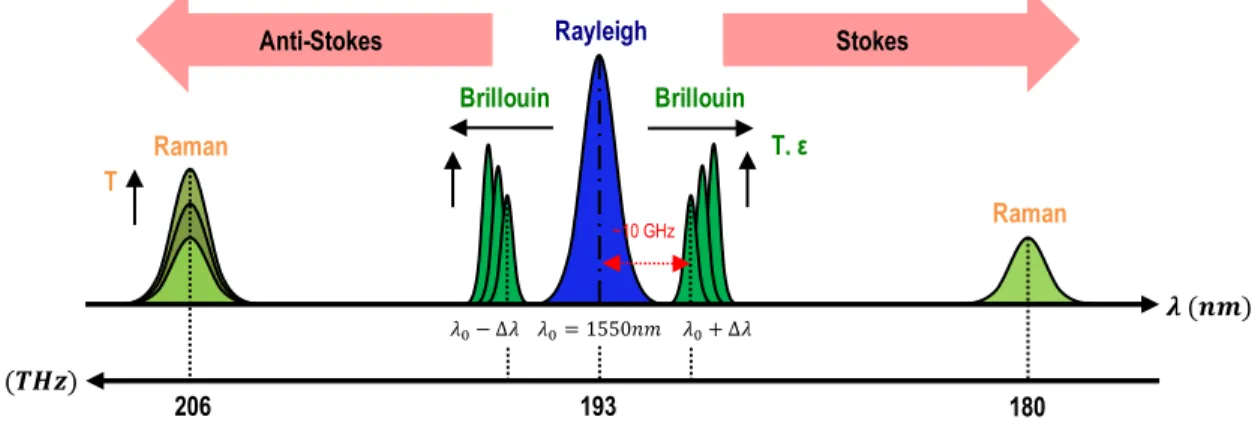
The three well-known scattering mechanisms occur within optical fibres, i.e. Rayleigh-, Raman-, and Brillouin-scattering, which is described in the Fig. 1.15 [49] with a standard single-mode fibre (SMF).
The Rayleigh scattering is an elastic process which preserves the incident photon energy that occurs through the interaction of light with inhomogeneities of a much smaller scale than the wavelength of the incident light. The presence of non-uniformity in RI along the fibre length due to the fluctuations of material density and composition of dopants causes small amount of the incident light to scatter in backward direction producing backscattering (refer to Fig. 1.16). In this way, the characteristics of backscattered light can be utilised to extract fibre information and subsequently determine ambient perturbations to which it is subjected to.
Raman- and Brillouin-scattering are inelastic processes in which the incident photon energy is not conserved, which means that there is an energy exchange between the incident light and the material; this results in a
Figure 1.15 Various scattering processes in a standard SMF showing Rayleigh, Raman, and Brillouin shifts with Stokes and anti-Stokes signals
Rayleigh Anti-Stokes Stokes 𝝀 (𝒏𝒎) 𝝂 (𝑻𝑯𝒛) Raman Raman Brillouin Brillouin T
ε
T, ε 𝜆·− ∆𝜆 193 180 206 ~10 GHz 𝜆·+ ∆𝜆 𝜆·= 1550𝑛𝑚 Cladding Cladding Core Microscopic-scale inhomogeneitiesfrequency shift of the scattered light. In inelastic scattering processes, the local RI variations are induced by thermally driven vibrations on phonons. The heat generation in the material results in molecule vibrations (stretching, bending or rotation of inter-atomic bonds) or lattice vibrations (longer-scale periodic movement of the material) [50].
Raman scattering is caused by molecule vibrations and its frequency shift is normally in the range of a few terahertz (THz) up to tens of THz depending on the molecule compositions. In case of a standard SMF, this frequency shift is in the range of ~10 THz, as shown in Fig. 1.15. It should be noted that the Raman Effect leads to two possible scattering mechanisms, which is shown in Fig. 1.17 [1]. When the energy of incident photons is transferred to the vibrational states of molecules, i.e. the energy is absorbed by the molecules, the scattered photons has a lower energy and its frequency is reduced. This process is labelled as Stokes bands due to the longer wavelength of light emitted. In contrast, when the vibrational energy of molecules is transferred to scattered photons, the process is referred to as anti-Stokes bands appearing at a shorter wavelength.
The anti-Stokes Raman operation depends on the population density of phonons involved in that process and its energy is strongly temperature-dependent, which is similar to the thermal energy ~𝑘¢𝑇 where 𝑘¢ is the Boltzmann constant and 𝑇 is the temperature. The intensity of anti-Stokes Raman peak is thus sensitive to the variation of temperature, which forms the working principle of Raman-based distributed optical fibre sensors (DOFSs).
In comparison with Raman scattering, the Brillouin scattering is originated from the lattice vibrations, i.e. phonons with low frequency in the hypersonic range of tens of gigahertz (GHz) [1]. In conventional SMFs, this frequency shift is in the range of 9~12 GHz (refer to Fig. 1.15) depending on fibre compositions of the core. In the same manner of Raman scattering, it can also bring out two outcomes, the Stokes or anti-Stokes Brillouin scattering
Figure 1.17 Energy diagrams of a) Stokes and b) anti-Stokes processes
Virtual energy level
Vibrational energy level
Stokes
Incident photon, 𝜐¹ Scattered photon, 𝜐x
𝜐· a) 𝜐¹ 𝜐x 𝜐· anti-Stokes b)
due to the energy transfer from incident light to vibrational modes of lattice or vice versa, respectively. The Brillouin frequency shift (BFS) is strongly dependent on temperature and strain, which establishes the basic principle in operating Brillouin-based DOFSs.
1.5 Permafrost system and related point sensors
Permafrost, by definition, is any type of frozen layer under the Earth’s surface down to from a few feet to more than 1 km. Usually, it consists of ground materials such as soil, rock, or sediment that bound together with ice, and remain at or below the temperature of 0°C for a minimum of two years [1]. It is mostly located in the norther hemisphere land covers a the huge area in Northern Canada, which is shown in Fig. 1.18.
Due to the temperature rise from global warming, the footprint of permafrost is rapidly shrinking. This process is expected to augment the global warming by 0.13-0.27°C by the year 2100 and 0.42°C by the year 2300 [51]. Several issues are associated with permafrost thawing that has given rise to some critical problems related to safety and security, human health, vulnerability of infrastructures and resource exploitation [52, 53]. One of the main concerns is the carbon release resulting from permafrost degradation, which has a potential important impact on the Earth’s climate system because the large amounts of carbon previously buried in frozen organic matters will decompose into greenhouse gases such as carbon dioxide (CO2), methane (CH4) or other pollutant
gases. These, in turn, contribute to the climate warming so that an unstoppable positive feedback loop is activated, which is explained schematically in Fig. 1.19 [52].
Globally, the temperature of permafrost was increased by 0.29±0.12°C, especially 0.39±0.15°C and 0.20±0.10°C rise in continuous and discontinuous permafrost zones, respectively, during the reference decade between the year 2007 and 2016 [51].
Another main issue from the permafrost degradation is the crumbling infrastructures, buildings and roads, causing severe impact to the local living environments and communities. Fig. 1.20 shows some examples of damaged infrastructures in the area of Northern Canada [53].
Furthermore, it can also alter the ecosystem and hydrological systems by causing the water pollution in local rivers, streams or lakes, degrading the water quality and impacting dramatically to aquatic wildlife. In addition, it tends to be exposed to the risk of disease due to the possibility of releasing ancient microbes (bacteria and viruses) trapped inside the permafrost for thousands of years [52].
Figure 1.19 A permafrost system and related occurrence during its thawing [52]
Figure 1.20 Examples of damaged infrastructures [53]
Active layer Transition layer
Surface temperature increases
Atmospheric CO2 and CH4 increase
Organic matters thaw and decay Permafrost
In order to systematically monitor the dynamic states of a permafrost system, three main physical changes including pore water pressure (PWP), temperature and displacement vertically along the permafrost, should be inspected as ultimate targets.
The PWP refers to the pressure of groundwater held within a soil or rock, in voids between particles (pores) and it is measured relative to the atmospheric pressure [1]. It plays an important role in geotechnical/civil engineering as it is closely related to safety and stability of geotechnical structures and civil infrastructures. Fig. 1.21 illustrates the PWPs in a hydrostatic-state soil environment. The natural static level of water in the ground is called the water table, at which the PWP is zero, which means it equals to atmospheric pressure [1].
Below the water table, the region saturated with water, the value of PWP becomes positive and simply calculated from the following formula,
𝑢 = ±𝛾¼ℎ (+𝑓𝑜𝑟 𝑝𝑜𝑠𝑖𝑡𝑖𝑣𝑒, − 𝑓𝑜𝑟 𝑛𝑒𝑔𝑎𝑡𝑖𝑣𝑒) (1.19)
where 𝛾¼ (9.8 kN/m3) is the unit weight of water and ℎ is the depth below the water table as indicated in Fig.
1.21. On the other hand, the PWP becomes negative (less than the atmospheric pressure) above the water table
Dry state Ground surface 𝒖 = −𝜸𝒘𝒉 𝒖 = 𝜸𝒘𝒉
-h
+h
Unsaturated (Negative) Saturated (Positive) Water table Borehole Soil environment De pt hFigure 1.21 An active layer in a soil environment showing the linear positive and negative PWPs depending on the water depth from the water table [52]
since the voids are partly filled with water and air through the capillary action. Nowadays, these positive/negative values of PWP are separately measured, respectively, with piezometer/tensiometer.
For measuring positive PWPs, there exist two main commercially available electrical piezometers, vibrating wire piezometer and electrical resistance piezometer. Fig. 1.22 illustrates the structure of a vibrating wire piezometer.
A flexible diaphragm separated from a porous filter by a water-filled reservoir. A tensioned wire is attached to the diaphragm on the opposite side to the reservoir, such that deflection of the diaphragm from water pressure leads to a change in the length of the wire, and hence the tension. As the pressure increases, the tension of the wire decreases, and vice versa. The tension in the wire is measured by setting it into vibration with a series of electromagnetic pulses from a coil. The wire then vibrates primarily as its natural resonant frequency. When excitation ends, the wire continues to vibrate and a sinusoidal signal, at the resonant frequency, is induced in the coil and transmitted to the readout unit. When the wire is vibrated through a magnetic field, the voltage across the ends of the wire varies with the length of the wire; the voltage can be measured and thus calibrated against the pressure of the water in the reservoir (RST Instruments).
The other popular one for measuring PWPs is the electrical resistance piezometer, also called strain gauge piezometer, whose operating design is schematically depicted in Fig. 1.23. A strain gauge is attached to a deflecting diaphragm. The water pressure applied to one side of the diaphragm through porous steel/ceramic filter causing the strain gauge to output a signal that is directly proportional to the applied stress. The induced piezo-resistivity is proportional to the stress applied to the diaphragm due to the deflection (RST Instruments).
Electrical coil
Tensioned wire Diaphragm
Water-filled reservoir Porous steel/ceramic filter Signal cable
Excluding those commercialised electrical piezometers, fiber-based interferometric and FBG point sensors have been proposed and explored to detect positive PWPs. Fig. 1.24 shows the fibres deployed and the transducers assembled in laboratory experiments for the case of in-line fiber interferometers [54].
Two types of polarization-maintaining photonic crystal fibers (PM-PCFs) have been employed to build the in-line fiber Sagnac interferometers as novel transducers to detect PWPs. Table 1.2 gives some specifications about the two test fibres.
PM-PCF (Blaze Photonics) SC-PM-PCF (Self-drawn) Core/cladding size Elliptical core size: 6.6 x 4.5 µm
Clad: 125 µm
Elliptical core size: 8 x 4 µm Clad: 125 µm
Two large holes: 4.2 µm 22 x 27 µm
Signal cable Electrical strain gauge
Water-filled reservoir
Diaphragm
Porous steel/ceramic filter
Figure 1.23 A structure of the electrical resistance piezometer
Figure 1.24 The PM-PCFs and transducers for in-line fiber interferometric point sensor measuring PWPs [54]
PM-PCF
SC-PM-PCF
Diameter of hole size Small holes: 2.2 µm
Intrinsic birefringence 4.2 x 10⁻⁴ 4.7 x 10⁻⁴
The established SI through the loop of a PM-PCF induces the corresponding spectrum that is mainly affected by the relative phase difference, which is sensitive to the surrounding pressure. The loop transmission spectrum can be expressed as,
𝑇 =[1 − 𝑐𝑜𝑠(𝛿)]
2 (1.20) where 𝛿 is the total phase shift of the Sagnac loop and it contains the intrinsic birefringence phase shift (𝛿·) and the pressure-induced birefringence phase shift (𝛿B) over the length (𝐿) of the PM-PCF. The total phase shift is described as [54],
𝛿 = 𝛿·+ 𝛿B =2𝜋𝐿
𝜆· {𝐵·+ 𝑘B∆𝑃~ (1.21) where 𝐵· is the intrinsic birefringence of the PM-PCF, 𝑘B is the coefficient of birefringence-pressure and applied pressure and ∆𝑃 is the change of surrounding pressure. When the sensor (refer to Fig. 1.24) is exposed to an environment with applied pressure, the parameter 𝛿B varies according to the applied pressure and it equals to 2𝜋 if the transmission minimum moves one full fringe to the adjacent one. Therefore, the total wavelength shift from the pressure-dependent birefringence is given by,
∆𝜆 =𝛿B 2𝜋∙
𝜆·•
𝐵·𝐿 (1.22) Combined with Eq. 1.21, the relationship between wavelength shift and applied pressure can be obtained as,
∆𝑃 = Ê 𝐵·
𝜆·𝑘BË ∙ ∆𝜆 (1.23)
This indicates that the applied pressure is linearly proportional to the spectral shift, which is the basic working principle for PM-PCF-based SI sensor. The resolution of the designed PWP sensor is about 3 kilopascal (kPa) when using the optical interrogator (SM125-500) with a scanning rate of 2 Hz and a wavelength resolution of 1 pm. The coefficient of wavelength-pressure of the commercial PM-PCF is 304.41 kPa/nm with the length of 35 cm as the sensing element while the coefficient of the SC-PM-PCF is 254.75 kPa/nm with the length of 100 cm. Therefore, it should be pointed out that more accurate PWP could be detected by using SC-PM-PCF with the

![Figure 1.25 The design of an FBG sensor for measuring PWP [55]](https://thumb-eu.123doks.com/thumbv2/123doknet/3068565.86635/42.918.220.708.557.810/figure-design-fbg-sensor-measuring-pwp.webp)


![Figure 2.13 An example of 3D-BGS as a function of the fibre length and detuning frequency [79]](https://thumb-eu.123doks.com/thumbv2/123doknet/3068565.86635/61.918.196.713.245.523/figure-example-bgs-function-fibre-length-detuning-frequency.webp)