O
pen
A
rchive
T
OULOUSE
A
rchive
O
uverte (
OATAO
)
OATAO is an open access repository that collects the work of Toulouse researchers and
makes it freely available over the web where possible.
This is an author-deposited version published in :
http://oatao.univ-toulouse.fr/
Eprints ID : 17105
The contribution was presented at EUSIPCO 2015 :
http://www.eusipco2015.org/
To cite this version :
Baussard, Alexandre and Tourneret, Jean-Yves Bayesian
parameter estimation for asymmetric power distributions. (2015) In: 23rd
European Signal Processing Conference (EUSIPCO 2015), 31 August 2015 - 4
September 2015 (Nice, France).
Any correspondence concerning this service should be sent to the repository
administrator:
[email protected]
BAYESIAN PARAMETER ESTIMATION FOR ASYMMETRIC POWER DISTRIBUTIONS
Alexandre BAUSSARD
(1,2)and Jean-Yves TOURNERET
(2)(1)
Lab-STICC (UMR CNRS 6285), ENSTA Bretagne, 2 rue Franc¸ois Verny, 29806 Brest c´edex 9, France.
(2)
IRIT (UMR CNRS 5505), INP-ENSEEIHT, 2 rue Charles Camichel, 31000 Toulouse, France.
ABSTRACT
This paper proposes a hierarchical Bayesian model for es-timating the parameters of asymmetric power distributions (APDs). These distributions are defined by shape, scale and asymmetry parameters which make them very flexible for ap-proximating empirical distributions. A hybrid Markov chain Monte Carlo method is then studied to sample the unknown parameters of APDs. The generated samples can be used to compute the Bayesian estimators of the unknown APD pa-rameters. Numerical experiments show the good performance of the proposed estimation method. An application to an im-age segmentation problem is finally investigated.
Index Terms— Asymmetric power distributions,
hierar-chical Bayesian model, MCMC, Gibbs sampler, Image seg-mentation.
1. INTRODUCTION
Many image processing applications require to define an ap-propriate probability distribution for the observed data. These applications include image classification, image segmenta-tion, image registration or change detection. A very classical approach for defining a probability density function (pdf) for observed data is to fit the empirical histogram of these data by classical pdfs such as Gaussian, gamma, Laplace or by their generalized versions. In particular, the symmetric general-ized Gaussian distribution has received a considerable atten-tion in the literature because it generalizes classical distribu-tions such as the Gaussian or Laplace distribudistribu-tions. However, in some other applications such as econometrics [1, 2] or im-age processing, asymmetry has been observed in the distribu-tion of the data. In particular, image processing applicadistribu-tions involving asymmetric distributions include segmentation of magnetic resonance images (MRI) [3] or texture classification using wavelet coefficients [4].
This paper studies asymmetric power distributions (APDs) that have been introduced in [1, 2]. These distributions are characterized by scale, shape and asymmetry parameters which make them more flexible than the symmetric distri-butions for approximating empirical histograms. We are particularly interested in developing a Bayesian parameter estimation method for this kind of distributions. More pre-cisely, all the unknown parameters of APDs are assigned prior distributions summarizing the known information about
these parameters. A Markov chain Monte Carlo (MCMC) method is then introduced to sample the resulting posterior distribution and to compute the Bayesian estimators of the unknown APD parameters. The performance of the proposed Bayesian estimation method is evaluated via several simula-tion results. An applicasimula-tion to the segmentasimula-tion of images with APDs is finally investigated.
The paper is organized as follows. The asymmetric power distributions considered in this work are introduced in Sec-tion 2. SecSec-tion 3 presents the Bayesian model suggested for estimating the APD parameters. The Bayesian estimators as-sociated with this model being difficult to compute in closed-form, we study in section 4 an MCMC approach that can be used to sample according to the posterior of the unknown APD parameters. The performance of this approach is evalu-ated via simulevalu-ated results associevalu-ated with synthetic data. Sec-tion 5 considers an applicaSec-tion of the proposed method for im-age segmentation. Section 6 gives some concluding remarks and future work.
2. ASYMMETRIC POWER DISTRIBUTIONS (APDS)
We consider a class of univariate asymmetric power distribu-tions defined by the following pdf
fAPD(x|θ) = δ1/λ γ1/λΓ(1+1/λ)exp ! − δ γαλ|x|λ " , if x ≤ 0 δ1/λ γ1/λΓ(1+1/λ)exp ! − δ γ(1−α)λ|x|λ " , if x > 0 (1) where θ= (λ, γ, α)T is a vector containing the APD param-eters,Γ(.) is the gamma function and δ = α2αλ+(1−α)λ(1−α)λλ.
The shape of the APD distribution is adjusted by the pa-rameterλ > 0 controlling the tail decay whereas α ∈ (0, 1) characterizes the degree of asymmetry andγ > 0 is a scale parameter. Some related APD definitions that are equivalent up to an appropriate change of variables can also be found in [1, 2, 4].
The proposed distribution defined by (1) has two main ad-vantages (for our purpose) with respect to APDs of [1] or [4]: the asymmetric parameter is constrained to belong to a finite length interval(0, 1) and the presence of a scale parameter makes it more flexible for practical applications.
3. BAYESIAN PARAMETER ESTIMATION
This section studies a Bayesian method for estimating the pa-rameters(α, λ, γ) of an APD. The motivation for using this method is that it is generic and can be applied to many prob-lems involving APDs. In particular, the image segmentation problem considered in Section 5 can be handled by a similar method. Conversely, the maximum likelihood method pro-posed in [1] cannot be easily applied to the image segmenta-tion problem which requires to estimate discrete and continu-ous parameters. The principle of parameter estimation using Bayesian inference is to define appropriate priors for the un-known parameters (and possibly hyperparameters) and to es-timate these parameters using their posterior distribution. The priors considered in this study are summarized below.
3.1. Prior distributions
According to the APD pdf given in equation (1), the shape pa-rameterλ is defined on IR+. However, in practical problems, its range can be reduced to[0, 3] [5]. Thus, one can assign to λ the uniform prior
p(λ) = 1
3 1I[0,3](λ). (2)
The scale parameter is assigned a Jeffreys prior p(γ) = 1
γ1IIR+(γ). (3)
This choice of non-informative prior is very classical for scale parameters (see [6] for motivations).
The asymmetry parameter α is constrained in the interval (0, 1). When there is no additional information, it is natural to choose the following uniform prior for this parameter
p(α) = 1I(0,1)(α). (4)
3.2. Posterior distribution
We assume that the parametersα, λ and γ are a priori in-dependent. For any sample x = (x1, ..., xn)T ∈ IRn dis-tributed according to an APD with unknown parameter vector θ= (λ, γ, α)T, the posterior distribution of θ can be written
p(θ|x) ∝ # n $ i=1 p(xi|θ) % p(λ)p(γ)p(α) (5) where∝ means “proportional to”. This posterior is too com-plex to derive closed-form expressions of the Bayesian esti-mators of θ. As a consequence, we propose to use an MCMC method to generate samples asymptotically distributed ac-cording to (5) and to use the generated samples to build estimators of the unknown parameters. It is the objective of the next section.
4. HYBRID GIBBS SAMPLER
The principle of MCMC methods is to construct a Markov chain whose equilibrium distribution is the target posterior distribution. In order to do that, the basic Gibbs sampler gen-erates samples according to the conditional distributions of the target distribution. When the conditional distribution of a subvector of the unknown parameter vector cannot be sam-pled easily, we can generate this subvector according to an appropriate proposal and accept or reject this generated vec-tor using the Metropolis acceptance ratio. When Metropolis moves are used inside a Gibbs sampler, the resulting MCMC method is referred to as Metropolis-within-Gibbs or hybrid Gibbs sampler. This strategy can be used to generate sam-ples distributed according to (5) by sampling according to the conditional distributions p(λ|x, γ, α), p(γ|x, λ, α) and p(α|x, λ, γ), which are detailed below.
4.1. Sampling the shape parameterλ
The conditional distribution of the shape parameterλ satisfies the following relation
p(λ|x, γ, α) ∝ p(x|θ)p(λ) (6) wherep(λ) has been defined in (2). As a consequence
p(λ|x, γ, α) ∝ & n $ i=1 p(xi|θ) ' p(λ) ∝ δ n/λ γn/λΓn(1 + 1/λ)1I[0,3](λ) × exp ( −δ||x −||λ λ γαλ − δ||x+||λ λ γ(1 − α)λ ) (7) where x+and x−
contain all the positive and negative sam-ples xi and||x||λ is the lλ-norm. Unfortunately, this con-ditional distribution is not easy to sample directly. Thus, a random walk Metropolis Hastings (MH) move is used [7]. This move requires to define an appropriate proposal, which has been chosen as a zero mean Gaussian distribution whose variance has been adjusted a priori to obtain a suitable aver-age acceptance ratior. In practice, a reasonable range of r is 30% to 90% and it is calculated within a sliding window of 30 samples. Note that to make sure the Markov chain is ho-mogeneous after the burn-in period, this tuning procedure is only executed in the burn-in period (see [8] for more details). The classical MH acceptance ratio necessary to ensure that the generated samples are asymptotically distributed ac-cording to their conditional distributions is
ρt= min * p(λ∗|x, γ, α) p(λt|x, γ, α), 1 + (8) whereλ∗
is the candidate generated for iterationt + 1 and λt is the value ofλ at iteration t.
4.2. Sampling the scale parameterγ
The conditional distribution of the scale parameterγ is p(γ|x, λ, α) ∝ p(x|θ)p(γ) ∝ &n $ i=1 p(xi|θ) ' 1 γ1IIR+(γ) ∝ 1 γnλ+1exp ( −1 γ , δ||x−||λ λ αλ + δ||x+||λ λ (1 − α)λ -) = IG, n λ, δ||x−||λ λ αλ + δ||x+||λ λ (1 − α)λ -(9) whereIG(a, b) is the inverse gamma distribution with hyper-parametersa and b.
Note that this distribution is easy to sample. This easy generation is mainly due to the form of APD introduced in (1), which differs from the definition of [2, 4].
4.3. Sampling the asymmetry parameterα
The conditional distribution of the asymmetric parameterα satisfies the following relation
p(α|x, λ, γ) ∝ p(x|θ)p(α). (10) Using the definition ofp(α) given in (4), the conditional dis-tribution can be written
p(α|x, λ, γ) ∝ & n $ i=1 p(xi|θ) ' p(α) ∝ δ n/λ γn/λΓn(1 + 1/λ)1I(0,1)(α) × exp ( −δ||x − ||λ λ γαλ − δ||x+||λ λ γ(1 − α)λ ) .(11) Since this conditional distribution is not easy to sample directly, we have used an MH acceptance rule based on a uniform proposal in the interval(0, 1). Again, the simple form of APD introduced in (1) makes this generation easier sinceα ∈ (0, 1) contrary to the APDs defined in [4] where α ∈ IR+.
4.4. Minimum mean-squared error estimation
The Bayesian estimators of the unknown parameters can be computed using the samples generated by the proposed hy-brid Gibbs sampler. More precisely, the generated samples are averaged after an appropriate burn-in period to compute the minimum mean-squared error (MMSE) estimators ofλ, γ andα.
4.5. Numerical simulations
Some numerical simulations have been run to evaluate the proposed estimation method. The first experiment considers
APD variates with parameters(λ, γ, α) that can be generated following the method proposed in [1], which is slightly mod-ified to account for the scale parameter.
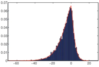
Fig. 1 shows an histogram of the generated datax1, ..., xn (blue histogram) corresponding to the parametersα = 0.75, λ = 1.3 and γ = 10. The distributions of the samples gen-erated by the proposed estimation algorithm are displayed in Fig. 2. The corresponding MMSE estimates± standard deviation, computed from 50 Monte Carlo runs, are ˆα = 0.748 ± 0.03, ˆλ = 1.297 ± 0.022 and ˆγ = 10.148 ± 0.628. These results are in good agreement with the true parameter values and confirm the good properties of the proposed Gibbs sampler. Finally, Fig. 1 also shows the good fit between the histogram of the generated data (in blue) and the APD pdf with the estimated parameters (in red).
−60 −40 −20 0 20 0 0.01 0.02 0.03 0.04 0.05 0.06 0.07
Fig. 1. Histogram of the generated APD random data (blue bars) and the corresponding estimated APD pdf (red line).
Fig. 2. Estimated marginal pdfs of the APD parameters.
5. APPLICATION TO IMAGE SEGMENTATION
This section shows that the algorithm developed before (to estimate the APD parameters) can be modified for an image segmentation application. More precisely, we assume that the image to be segmented is composed of homogeneous regions defined by different sets of APD parameters (α, λ, γ). The first part of this section describes the different steps of the proposed segmentation algorithm.
5.1. Problem formulation
Assuming the image is made up byK homogeneous regions, a label vectorz ∈ {1, ..., K}nmapping each image pixel into the set{1, ..., K} is defined. The distribution of the pixel xi
conditionally on thekth class is supposed to be defined as xi|zi= k ∼ AP D(θk) (12) where the APD parameter vector θ = (λ, γ, α)T is associ-ated with thekth class. Assuming the pixels are independent conditionally to the knowledge of their classes, we obtain the following prior for the target image
p(x|z, θ) = K $ k=1 nk $ i=1 fAP D(xi|zi= k, θk) (13)
where nk is the number of pixels in class #k and θ = (θT1, ..., θ
T K)T.
The prior of the image labels is supposed to be a Markov ran-dom field (MRF) to take advantage of the dependencies be-tween neighbor pixels in the image. The conditional distribu-tion ofzifor an MRF is defined as
p(zi|z−i) = p(zi|zν(i)) (14) where z−i= (z1, ..., zi−1, zi+1, ..., zi) and ν(i) contains the neighbors of labelzi. The whole set of random variableszi forms a random field. The Potts Markov field defined by the neighborhood structure (14) is particularly adapted to label-based segmentation [9]. Using the Hammersley-Clifford the-orem [10], the prior of z can be expressed as a Gibbs distri-bution p(z) = 1 C(β)exp[Φβ(z)] (15) with Φβ(z) = n . i=1 . i′∈ν(i) βδ(zi− zi′) (16)
whereβ is the granularity coefficient, δ(.) is the Kronecker function andC(β) is the normalizing constant. In this paper the value ofβ has been fixed to 1.2 by cross validation.
The image segmentation problem addressed in this paper consists of estimating the label vector z and the parameter vectors θk fork = 1, ..., K from the image x. We propose to study Bayesian estimators of(θ, z) based on the following posterior distribution p(z, θ|x) ∝ p(x|z, θ)p(z)p(θ) (17) with p(θ) = K $ k=1 p(θk) = K $ k=1 [p(λk)p(γk)p(αk)] . (18)
The posterior (17) is too complex to derive closed form ex-pressions of the Bayesian estimators of(θ, z). As a conse-quence, we propose to sample p(z, θ|x) by using a hybrid Gibbs sampler presented in the next section.
5.2. Hybrid Gibbs sampler
After an appropriate initialization, the proposed hybrid Gibbs sampler is made of4 steps
1. Sampling the shape parameter vector λ= (λ1, ..., λK)T 2. Sampling the scale parameters γ= (γ1, ..., γK)T 3. Sampling the asymmetry parameters α= (α1, ..., αK)T 4. Sampling the labels z
The first three sampling steps are very similar to those pre-sented in Section 4. The only modification appears in the expression of the conditional distributions which depend on the different labels. For example, the conditional distribution of the shape parameterλkcan be written
p(λk|xk, zk, αk, γk) ∝ p(xk|zk, θk)p(λk) with p(xk|zk, θk) = nk $ i=1 p(xi|zi= k, θk).
The last sampling step is required to define the conditional distribution of the label vector z. Following [8], the condi-tional distribution of the labels z can be computed using the Bayes rule
p(z|x, θ) ∝ p(x|z, θ)p(z). (19) Considering the dependency between a label and its neigh-bors, the conditional distribution of the labelzi (correspond-ing to image pixelxi) is given as follows
p(zi= k|z−i, x, θ) ∝ p(xi|zi= k, θ)p(zi= k|zν(i)). Denoting asπi,k= p(zi= k|z−i, x, θ), the normalized con-ditional probability of the labelziis
˜ πi,k = πi,k /K k=1πi,k . (20)
The labelzican be drawn from the set{1, ..., K} with the re-spective probabilities{˜πi,1, ..., ˜πi,K}. Note finally that a four-pixel neighborhood structure has been adopted in this paper.
5.3. Experiments
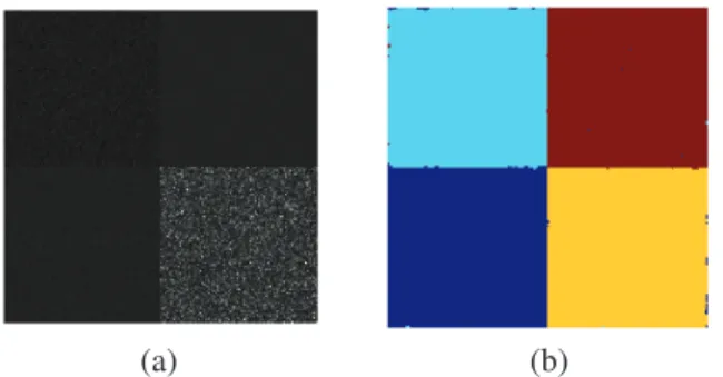
The proposed algorithm has been applied to a synthetic im-age composed of four areas defined by APDs with different parameters reported in Table 1. Each area contains100 × 100 pixels yielding an image of200 × 200 pixels. An example of a generated image using the considered APD parameters is displayed in Fig. 3 (a). The corresponding segmentation map obtained with the proposed algorithm is shown in Fig. 3 (b). It is clearly in good agreement with the ground truth (the rate of correct segmentation is equal to 99.7%).
Table 2 provides more quantitative results in term of means and standard deviations for the estimated APD parameters computed from50 Monte Carlo runs with the same param-eter values. From these results, after comparing the true and
Area 1 Area 2 Area 3 Area 4 α 0.75 0.35 0.5 0.15
λ 1.5 2 1.7 1.2
γ 10 2 5 15
Table 1. APD parameters of the areas of the synthetic image.
(a) (b)
Fig. 3. Representative example of (a) a synthetic image made of four areas with different APD parameters (as indicated in Table 1) and (b) a segmentation result.
the estimated parameter values, one can wonder whether the estimation is correct and effective, especially for the largest values ofγ. To illustrate this accuracy, Fig. 4 compares the histograms of the generated data for each area (blue bars) with the theoretical marginal posterior distributions (in red) and the estimated marginal posterior distribution (in green). Even if there are some differences between the estimated and the true parameter values, the green curves are superimposed with the red curves showing that the estimated APD parameters pro-vide a very good data fit.
Area 1 Area 2 Area 3 Area 4 ˆ α 0.756±0.003 0.346±0.003 0.498±0.003 0.138±0.002 ˆ λ 1.613±0.035 2.128±0.054 1.843±0.043 1.268±0.024 ˆ γ 12.580±0.956 2.075±0.089 6.101±0.417 17.254±1.343
Table 2. Estimated APD parameters for each image area.
6. CONCLUSIONS
This contribution proposed a new Bayesian model for esti-mating the parameters of an asymmetric power distribution. A Gibbs sampler allowing the parameters of this model to be generated was also studied. An application to image segmen-tation was finally investigated. The obtained simulation re-sults showed the efficiency of the proposed estimation method approach for both parameter estimation and image segmen-tation. Future work will be devoted to the analysis of real images with the proposed Bayesian framework.
REFERENCES
[1] I. Komunjer, “Asymmetric power distribution: Theory and applications to risk measurement,” Journal of
ap-plied econometrics, vol. 22, pp. 891–921, 2007.
Fig. 4. Marginal posterior distribution from the estimated (green) and true (red) APD parameters in each area of the image in Fig. 3.
[2] D. Zhu and V. Zinde-Walsh, “Properties and estimation of asymmetric exponential power distribution,” Journal
of econometrics, vol. 148, pp. 86–99, 2009.
[3] N. Nacereddine, S. Tabbone, D. Ziou, and L. Hamami, “Asymmetric generalized gaussian mixture models and EM algorithm for image segmentation,” in
Interna-tional Conference on Pattern Recognition, Istanbul, Turkey, 2010.
[4] N-E. Lasmar, A. Baussard, and G. Le Chenadec, “Asymmetric power distribution model of wavelet sub-bands for texture classification,” Pattern Recognition
Letters, vol. 52, pp. 1–8, 2015.
[5] L. Chaˆari, J-C. Pesquet, J-Y. Tourneret, Ciuciu P., and A. Benazza-Benyahia, “A hierarchical Bayesian model for frame representation,” IEEE Trans. Signal
Process-ing, vol. 58, no. 11, pp. 5560–5571, 2010.
[6] C. P. Robert and G. Casella, Monte Carlo Statistical
Methods, Springer Texts in Statistics, 2004.
[7] W. K. Hastings, “Monte Carlo sampling methods using Markov chains and their applications,” Biometrika, vol. 57, no. 1, pp. 97–109, 1970.
[8] N. Zhao, A. Basarab, D. Kouame, and J-Y. Tourneret, “Joint segmentation and deconvolution of ultrasound images using a hierarchical Bayesian model based on generalized Gaussian priors,” submitted to IEEE Trans.
Image Processing, 2015.
[9] M. Pereyra, N. Dobigeon, H. Batatia, and J-Y. Tourneret, “Estimating the granularity coefficient of a Potts-Markov random field within a Markov chain Monte Carlo algorithm,” IEEE Trans. Image
Process-ing, vol. 22, no. 6, pp. 2385–2397, 2013.
[10] J. Besag, “Spatial interaction and the statistical analy-sis of lattice systems,” Journal of the Royal Statistical