Air traffic control radar interference event in the Galileo E6 band: Detection and localization

an author's https://oatao.univ-toulouse.fr/27101

https://doi.org/10.1002/navi.310

Arribas, Javier and Vilà-Valls, Jordi and Ramos, Antonio and Fernández͈Prades, Carles and Closas, Pau Air traffic control radar interference event in the Galileo E6 band: Detection and localization. (2019) Navigation, 66 (3). 505-522. ISSN 0028-1522

Air traffic control radar interference event in the Galileo E6

band: Detection and localization

Javier Arribas

Jordi Vilà-Valls

Antonio Ramos

Carles Fernández-Prades

Pau Closas

1_{Statistical Inference for Communications}

and Positioning Department, Centre Tecnològic de Telecomunicacions de Catalunya (CTTC/CERCA), Barcelona, Spain

2_{ISAE-SUPAERO, University of Toulouse,}

Toulouse, France

3_{Electrical and Computer Engineering}

Department, Northeastern University, Boston, Massachusetts

Correspondence

Javier Arribas, Statistical Inference for Communications and Positioning Department, Centre Tecnològic de Telecomunicacions de Catalunya (CTTC/CERCA), 08860, Barcelona, Spain. Email: jarribas@cttc.es

Funding information

Generalitat de Catalunya, Grant/Award Number: 2017-SGR-1479; Ministerio de Economía y Competitividad, Grant/Award Number: TEC2015-69868-C2-2-R (ADVENTURE); National Science Foundation (NSF) under Grant/Award Numbers: CNS-1815349 and

ECCS-1845833

Abstract

The Galileo E6 band operates at a nonprimary frequency band within the L-band. This presents challenging situations in the vicinity of other, legitimate, radiolocation services. This is the case for Air Traffic Control (ATC) radar, which is seen as an in-band–pulsed interference by a GNSS receiver. This paper pro-vides a detailed study of the impact of such interference, as well as localization approaches. Particularly, the paper describes the ATC jamming event captured on a GNSS permanent station, its effects on a real receiver, and how it was tracked to localize the source of interference. An ultra low-cost array-based solu-tion is prototyped, based on commercial off-the-shelf devices, that implements a two-element array. Experimental results are shown and discussed using real data, validating the localization performance of the prototype.

1

I N T RO D U CT I O N

The vulnerability of Global Navigation Satellite Sys-tems (GNSS) to Radio Frequency Interferences (RFI), either intentional or unintentional, is a fact widely studied in recent times.1 _{The performance degradation} and even the denial-of-service situations are especially important for safety-critical operations, such as aero-nautical high-accuracy positioning and navigation or for distributed timing services, where availability, integrity, and accuracy are mandatory. One of the most powerful unintentional interference sources comes from radionavi-gation aids. In particular, the civil air traffic control (ATC)

primary and secondary surveillance radars operated in the L-Band (1250 to 1350 MHz) are very close to the Galileo E5 (1189 MHz) and GPS L5 (1207.140 MHz) bands. Because of their high power-pulsed transmissions, which can reach values of tens of kilowatts, they are disrupting the GNSS service, as reported in previous studies.2-5_{The ATC} inter-ference in the Galileo E5 and GPS L5 bands represents an out-band interference that can be mitigated, for instance, using sharper bandpass filters in the receiver front-end.4

In February 2017, the European Commission and the European GNSS Agency (GSA) confirmed that the first generation of Galileo satellites would already provide users with high accuracy and authentication services on the

Galileo E6 band (1260 to 1300 MHz), referred to as Galileo commercial service (CS).6 _{The ATC radar interference is} particularly due to the following facts:

• The Galileo E6 band is completely overlapped with the

ATC L-Band, which produces a strong-pulsed in-band interference that cannot be mitigated using an antenna filter. This is especially problematic if the receiver uses a multi-band antenna (such as E1/L1 + E5/L5 + E6).

• The current International Telecommunication Union

(ITU) regulations7 _{and the European radiofrequency} spectrum regulation consider radionavigation aids and the GNSS service as co-primary users. However, in the European Conference of Postal and Telecommu-nications Admistrations (CEPT),8 _{it is recommended} that GNSS shall not interfere with radionavigation aids (see note 5.329), which provides the latter with higher priority.

• The existing legacy ATC L-Band radars, which should

be progressively migrated to the S-Band, are still in their medium lifespan.

The confluence of these factors guarantees the persis-tence of the interference for several years in the future. The authors detected such a situation in Spain, in the Barcelona metropolitan area during their daily research activity. The same problem is likely to occur in other locations all over Europe, representing a real threat that needs to be seriously taken into account. This contribu-tion reports a real ATC radar interference and its impact on GNSS receivers. Together with the detection and anal-ysis of the unintentional ATC radar jamming, an ultra low-cost array-based solution for interference localization is proposed, which is composed of two elements that esti-mate azimuth of the interference signal. Notice that in addition to the results provided in this article, the

mitiga-tion of such interference can be easily implemented via a real-time pulse blanking algorithm,9_{as was done in a} pre-vious contribution by the same authors,10_{where a single} antenna setup and an open source software-defined GNSS receiver11_{were considered.}

The paper is organized as follows. Section 2 describes an ATC radar interference event detected in the Barcelona metropolitan area that was reported by the authors to the national radio frequency management authorities due to its critical impact in GNSS. Section 3 adresses the impact and mitigation of the ATC radar interference. Section 4 briefly discusses the antenna array signal model for an arbitrary interference waveform, describing an inter-ference detection algorithm and a signal direction of arrival (DOA) estimation method. Section 5 proposes a maximum likelihood (ML) estimation-based triangulation algorithm for interference location, using a set of DOA estimations. The implementation of a prototype based on software-defined radio (SDR) technology is described in Section 6, including synchronization challenges in low-cost devices. Section 7 shows the algorithm imple-mentation validation by simulations, and Section 8 shows the results obtained in a real-life measurement campaign to detect and localize the ATC radar-pulsed interference. Finally, Section 9 concludes the paper.

2

ATC R A DA R I N T E R F E R E N C E

E V E N T

In February 2016, the GESTALT® (GNSS SignAL Testbed) lab facility (see Arribas et al12 _{for a detailed description} of the GNSS hardware and software set) located at the Centre Tecnològic de Telecomunicacions de Catalunya (CTTC) headquarters in Castelldefels (Barcelona, Spain) was used to capture and analyze the new Galileo E6 signals

FIGURE 1 GNSS band frequency allocation (source: http://www.navipedia.net/) [Color figure can be viewed at wileyonlinelibrary.com and www.ion.org]

ARRIBASET AL. 507

FIGURE 2 GESTALT® Testbed for experimentation with GNSS signals. It includes a set of antennas and a rack housing RF front-ends, measurement equipment, and a host server running instances of an open source software-defined GNSS receiver [Color figure can be viewed at wileyonlinelibrary.com and www.ion.org]

transmitted in the RF band from 1260 to 1300 MHz, as shown in the GNSS frequency allocation diagram of Figure 1.

For the experiment, we used a geodetic-grade GNSS-active antenna NavXperience 3G+C (E1, E5a, E5b, E5a+b, E6 band support) located on a platform at the roof of CTTC headquarters, as shown in Figure 2. The RF front-end was a USRP X310 equipped with an SBX daugh-terboard, tuned at 1278.75 MHz with a sampling rate of 20 MSps.

The time analysis revealed a concerning situation: The signal was severely interfered by an unknown pulsed inter-ference, as shown in Figure 3. The pulse power was orders

FIGURE 3 Galileo E6 signal with the presence of unknown pulsed interference [Color figure can be viewed at

wileyonlinelibrary.com and www.ion.org]

of magnitude stronger than the thermal noise floor as shown in Figure 4. A zoom plot, available in Figure 5, shows that each pulse had a chirp-shaped waveform.

In order to measure the interference power and its fre-quency signature, a spectrum analyzer was used to explore the complete GNSS band and its neighborhood. Figure 6 shows an exploration from 1 to 1.6 GHz. This analysis revealed two predominant peaks located at 1.2655 GHz (shown again in Figure 7), with −62.78 dBm, and 1.321 GHz with −68.26 dBm. Both time and frequency anal-ysis results indicated that the most likely source of the interference was an ATC radar. The interference signa-ture matched the L-band ATC primary radar spectral

FIGURE 4 Galileo E6 pulsed interference periodicity [Color figure can be viewed at wileyonlinelibrary.com and www.ion.org]

FIGURE 5 Galileo E6 single pulse interference time analysis [Color figure can be viewed at wileyonlinelibrary.com and www.ion.org]

characteristics described in Angelis et al.2 _{The last clue} to finding the interference source was obtained by doing a visual search in the surroundings of the affected GNSS antenna. Figure 8 shows a picture taken from the GNSS antenna location revealing Barcelona's airport ATC radar in the receiver's line of sight. It is important to highlight that this situation was not a single isolated event, but sustained over time due to the ATC radar continuous oper-ation. The interference was still present in the latest tests performed in December 2018.

Because of the critical impact of such interference into the GNSS E6 band, a report was sent February 2016 by the authors to the Spanish national radio frequency

FIGURE 6 Radio frequency (RF) spectrum at the antenna connector [Color figure can be viewed at wileyonlinelibrary.com and www.ion. org]

management authorities and an official investigation was performed. Notably, according to the 2016 European Table of Frequency Allocations (see CEPT,8p. 101_{), the service}

allocation for the range of 1270 to 1300 MHz reads: 1. Earth exploration satellite (active)

2. Radiolocation

3. Radionavigation satellite (space-to-Earth) 4. Space research (active)

5. Amateur

The listing order indicates the service priority, and thus, the ATC radar (a radiolocation service) has priority over the satellite radionavigation service. Consequently, the interference will be present until L-band radars end their operational life and migrate to S-band radars (as is fore-seen for next generation ATC), which means that this type of unintentional interference may still be present in some locations for the next decade.

Single-frequency GNSS antennas are usually equipped with Surface Acoustic Wave (SAW) filters, which provide strong out-of-band attenuation to interferences and pro-tect the front-end from saturations. However, in the case of antennas in the E6 band, the radar interference becomes an in-band interference (seen from the antenna device), in which case the antenna cannot filter out this signal and it is received with full power into the RF front-end.

Additionally, the ATC radar signal also affects other navigation bands, as a strong out-of-band interference. General-purpose tunable front-ends, like the Analog Devices AD13 _{are typically very sensitive to out-of-band} interferences due to the lack of selectivity of their tunable

ARRIBASET AL. 509

FIGURE 7 Spectrum detail of the 1.2655 GHz interference [Color figure can be viewed at wileyonlinelibrary.com and www.ion.org]

FIGURE 8 Barcelona L-band air traffic control (ATC) primary radar in the Global Navigation Satellite Systems (GNSS) receiver line of sight [Color figure can be viewed at wileyonlinelibrary.com and www.ion.org]

filters. Even by tuning the front-end to the L1/E1 band, it does not protect the input amplifiers and mixers from saturation due to the interference power. The effects are new intermodulation products, which affect all GNSS bands, thus, the out-of-band interfer-ence becomes an in-band interferinterfer-ence. SDR receivers are commonly connected to such front-ends, and thus it is specially important to assess the interference impact to SDR GNSS receivers and implement countermea-sures to minimize such interference effects, as reported

in Arribas et al.10 _{For completeness, we provide such} impact and mitigation analysis in the following section.

3

I M PACT A N D M I T I GAT I O N O F

T H E ATC R A DA R I N T E R F E R E N C E

I N S D R G N S S R EC E I V E R S

As already stated, when using SDR GNSS receivers in the L1/E1 band with general purpose front-ends, the ATC

FIGURE 9 Galileo E1 signal interfered by ATC radar pulses (top), and the same input signal after pulse blanking (bottom) [Color figure can be viewed at wileyonlinelibrary.com and www.ion.org]

FIGURE 10 Tracking results with the open source GNSS-SDR receiver for Galileo E1 under radar interference [Color figure can be viewed at wileyonlinelibrary.com and www.ion.org]

ARRIBASET AL. 511

FIGURE 11 Tracking results with the open source Global Navigation Satellite System software-defined radio (GNSS-SDR) receiver for Galileo E1 under radar interference, considering a pulse blanking filter with probability of false alarm = 0.04 [Color figure can be viewed at wileyonlinelibrary.com and www.ion.org]

radar interference in the E6 band may appear as an out-of-band interference. This is clear from the top plot in Figure 9 for a Galileo example, where the out-of-band pulses are leaking from E6 to E1. These radar pulses cause spurious correlation spikes at the acquisition and tracking stages of the receiver.

To assess the impact of the real ATC radar interference into an SDR GNSS receiver, we consider the use of an open source software defined GNSS receiver.11 _{We show} the tracking results for 53 seconds of signal in Figure 10. In this case, the receiver is not able to correctly track the signal (continuous loss-of-lock) because the pulses cause spikes in the early-prompt-late correlators. The top plots in Figure 10 show that the navigation data bits (BPSK) are not decoded, thus the receiver is not able to provide a PVT solu-tion due to the radar interference, thus a complete GNSS service denial results.

An easy countermeasure for such interference is to use a pulse blanking algorithm.9 _{An example of the blanked} signal is shown in the bottom plot in Figure 9, where the pulses have been effectively filtered. Using the blanking filter considerably improves the signal quality.

The tracking results considering a real-time pulse blank-ing filter with a false alarm of 0.04 are shown in Figure 11. In this case, the navigation message is correctly decoded (see the BPSK data bits in the top plots) and the receiver provides a PVT solution, with a time to first fix of 42 seconds. Only one pulse at second 32 is not blanked,

but this does not break the correct receiver operation. The present contribution extends the preliminary analysis in Arribas et al10 _{and proposes a low-cost antenna array} prototype made with off-the-shelf components and SDR tools, with the main goal being to gather DOA measure-ments of the interference source, which will be used in the DOA-based localization algorithm.

4

I N T E R F E R E N C E D ET ECT I O N

A N D D OA E ST I M AT I O N

Considering that a GNSS interference signal is received with an N-element antenna array, the discrete baseband signal model can be defined as

X(t) = hdint(t) +N(t), (1)

where:

• X(t) = [x(t−(K −1)Ts), … , x(t)] ∈CN×Kis referred to as

the space-time data matrix, where x(t) = [x1(t) … xN(t)]T

is defined as the antenna array baseband snapshot; each row corresponds to one antenna and K is the number of captured snapshots. The snapshot time interval can be defined as Tsnap=KTswhere Fs=1∕Tsis the sampling

frequency.

• h = [h1, … , hN]⊤∈CN×1is the non-structured channel

model, which includes both the channel and the array response. The channel vector assumes the role of the spatial signature but does not impose any structure. The

arbitrary structure of h, which is considered constant during Tsnap, is not only parameterized by the

interfer-ence signal DOA and the location of antennas, but also may include other unmodeled phenomena.

• dint(t) = [s(t − (K −1)Ts−𝜏), … , s(t − 𝜏)] ∈C1×Kis the

discrete version of the interference signal with an arbi-trary waveform, such as the pulsed interference shown in Figure 5.

• N(t) = [n(t − (K − 1)Ts) …n(t)] ∈ CN×K is a

complex, circularly symmetric Gaussian vector process with zero-mean, temporally white, and spatially white assuming:

E{n(tn)} =0, (2)

E{n(tn)n⊤(tm)} =0, (3)

E{n(tn)nH(tm)} =𝜎2I, (4)

where E{·} is the expectation operator, it is assumed that the noise has double-sided spectral density𝜎2₌ N0

2

W/Hz, and I stands for the identity matrix.

For the purpose of this study, and due to the low GNSS signal power available at Earth's surface, GNSS signals can be assumed to be well below the noise floor and, therefore, their contribution can be considered as Gaussian noise and included in the thermal noise term.14

The first step of an interference localization system con-sists of determining if the interference is present inside the receiver's band. From a computational point of view, a simple method is to compute the input signal power and compare it against a certain threshold. This threshold should be set according to the signal level in absence of the interference signal. Since the power of GNSS useful signal components at the receiver's antenna is extremely weak (several tens of dB below the background noise), the input signal power when the interference source is switched off is in practice the same as the background noise power, defined as

E{|xi[n]|2

}

≃𝜎2. (5)

After the analog-to-digital converter (ADC) step, and exploiting the statistical properties of n, it is possible to set a probability of false alarm, ie, the probability of detect-ing the interference even if the jammdetect-ing signal is absent. Comparing the signal magnitude against the threshold and taking a decision in all the samples is not feasible in real time applications, so the detection algorithm runs on sig-nal segments of L samples. The estimated energy of a sigsig-nal segment at the ith antenna element is

Ei= L

∑

k=1

|xi[k]|2, (6)

where the random variable Ei

𝜎2 follows a chi-square

dis-tribution with 2L degrees of freedom. According to the

tabulated values of such a distribution, it is possible to set the threshold with a certain probability of false alarm. When the segment's energy exceeds the detection thresh-old, the segment might contain an interference, and it is processed with the DOA estimation algorithm. Note that 𝜎2 _{should be estimated with a noise floor power}

estima-tion method. With the purpose of minimizing random effects, several noise power estimations are averaged on consecutive signal segments. In addition, as the receiver background noise may change over time, the estimation of 𝜎2_{is performed periodically.}

Considering a calibrated array, several algorithms can be used to estimate the interference signal DOA. In this contribution, we selected the well-known spectral Multi-ple Signal Classification (MUSIC) algorithm.15, p.1158 _The

MUSIC test function can be defined as ̂𝜃 = arg max

𝜃

1

v(𝜃)H_{(I − uu}H_)v(𝜃), (7)

where v(𝜃) ∈ CN×1 _{is the signal steering vector defined}

by its azimuth𝜃, u ∈ CN×1_{is the eigenvector associated}

with the most powerful eigenvalue of ̂Rxx = _K1XXH, and

I ∈RN×N_{stands for the identity matrix.}

Notice that in the experimental prototype described in Section 6, we have considered an array composed of N = 2 elements. As a consequence, only the interference azimuth,𝜃 ∈ [0◦, 180◦), is considered, with an ambiguity of 180◦.

Assuming the signal model defined in Equation 1,

E{ ̂Rxx} = U𝚲UH, where U is a unitary matrix

whose columns are the eigenvectors of Rxx and 𝚲 =

diag{𝜆1, … , 𝜆N}, where𝜆iis defined as the corresponding

eigenvalue. The most powerful eigenvalue and its eigen-vector are associated with the interference subspace as follows: 𝜆int =E {₁ Kdintd H int } (8) uint=h. (9)

If there is only one interference impinging into the array, the rest of eigenvalues are𝜆noise≈𝜎2. Besides the

interfer-ence detection based on the energy estimation described in Equation 6, it is also possible to define a new test statistics based on the difference between eigenvalues as follows:

𝛾dB=10log10 ( 𝜆max 𝜆min ) , (10)

where 𝜆max and𝜆min stands for the maximum and

min-imum eigenvalues of ̂Rxx, respectively. If there is only

one interference impinging into the array, then,𝛾dBis an

ARRIBASET AL. 513

5

I N T E R F E R E N C E

LO C A L I Z AT I O N A LG O R I T H M

The bearings-only interference localization can be formu-lated as a maximum likelihood (ML) estimation problem.16 The goal is to obtain the ATC radar static position, p = [p_x, p_y]⊤ from a set of M noisy estimated bearings, ̂𝜽 = [ ̂𝜃1, … , ̂𝜃M]⊤. The ith estimated measurement ̂𝜃i is

com-puted at a sensor (array) known position, ri = [rx,iry,i]⊤.

Then the true bearing angle is defined as 𝜃i(p) = tan−1 ( p_𝑦−r_𝑦,i px−rx,i ) , (11)

and 𝜽(p) = [𝜃1(p), … , 𝜃M(p)]⊤. The ith estimated

bearing—obtained from (7)—can be modeled as a noisy version of the true angle,

̂𝜃i=𝜃i+ni, ni∼

( 0, 𝜎2ni

)

, (12) where the measurement noise is assumed to be Gaussian and independent across estimations. Considering the vec-tor of M estimated bearings ̂𝜽, the M × M measurement error covariance matrix is C = diag(𝜎2

n1, … , 𝜎

2

nM), then the log-likelihood function, ln𝑓(̂𝜽|q), can be written as

−1 2ln ( (2𝜋)M_det(C))₋1 2(̂𝜽−𝜽(q) )⊤ C−1(̂𝜽_−𝜽(q)) ₍₁₃₎

where q ∈ R2 _{represents the two-dimensional target}

location. Maximization of the log-likelihood function is equivalent to minimizing the cost function

JML(q) = 1 2(̂𝜽−𝜽(q) )⊤ C−1(̂𝜽−𝜽(q)) = M ∑ i=1 1 2𝜎2 ni ( ̂𝜃i−𝜃i(q) )2 . (14)

The ML estimator of the ATC radar position is then given by ̂pML=arg min q∈R2JML(q)⇒ 𝜕JML(q) 𝜕q ||||q=̂pML =0, (15) which is a nonlinear minimization problem and has no closed-form solution. We use an iterative procedure to opti-mize the cost function. The gradient of the cost function is given by 𝜕JML(q) 𝜕q = M ∑ i=1 𝜃i(q) − ̂𝜃i 𝜎2 ni||q − ri|| [ −sin(𝜃i(q)) cos(𝜃i(q)) ] , (16)

and we can use a steepest-descent algorithm to recursively obtain the ML estimate of the radar position as

̂pk+1= ̂pk−𝜇𝜕JML

(q)

𝜕q ||||q=̂pk

, (17) where ̂p0 is the radar position initialization and𝜇 > 0 a

small positive step size.

6

P ROTOT Y P E I M P L E M E N TAT I O N

The idea of using extremely cheap RF front-ends to receive GNSS signals was already explored in Arribas et al,17_where the goal was to use a digital television front-end USB don-gle to successfully obtain a position fix by adapting the open-source GNSS-SDR. The so-called RTLSDR receiver with a retail cost below US $25 is based on Taiwan's Real-tek RTL2832U DVB-T receiver chipset, sold in the form of USB dongles that allow users to watch over-the-air DVB-T European broadcast television on their personal comput-ers (see Figure 12). Those devices send partially-decoded MPEG transport frames over the USB, but by exploiting an undocumented mode of operation of the demodulator chip, the user is able to obtain raw I&Q samples, stream them through USB to a personal computer and then apply the GNSS-SDR software processing.17

At that time, in September 2013, Juha Vierinen, a researcher involved in the Kilpisjärvi Atmospheric Imag-ing Receiver Array (KAIRA), Finland, did an experiment with two RTLSDR's dongles, modified for sharing the same reference clock source.18_{The hardware modification} con-sisted of removing the 28.8 MHz XTAL in one of the don-gles (see Figure 12) and connecting the clock input directly to the other dongle XTAL signal output. Apparently, the two front-ends are synchronized in both the downconver-sion chain and in the baseband sampling process. How-ever, due t the independent USB transport streams and different sampling start times, both sample streams are not synchronized as seen from the SDR software running in the CPU, resulting in a time shift between channels, con-stant in time during the capture or processing session but random over sessions.

FIGURE 12 RTLSDR dongle with onboard reference clock [Color figure can be viewed at wileyonlinelibrary.com and www.ion.org]

FIGURE 13 Ultra low cost antenna array prototype with N = 2 elements [Color figure can be viewed at wileyonlinelibrary.com and www.ion.org]

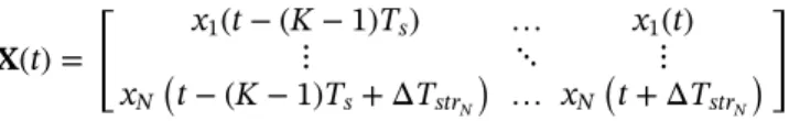
Considering the array signal model in Equation 1, it is possible to model the RTLSDR sample stream misalign-ment as follows: X(t) = [ _x 1(t − (K −1)Ts) … x1(t) ⋮ ⋱ ⋮ xN ( t − (K −1)Ts+ ΔTstrN ) … xN ( t + ΔTstrN ) ]

where ΔTstri =KstriTsis the random time delay present in the ith array channel equivalent to an integer number of samples Kstri.

Some time later, in 2015, Piotr Krysik, who wanted to use a set of RTLSDRs to receive multiple GSM frequency chan-nels at a time, published a GNU Radio Companion (GRC) block19 _{that effectively performs a time synchronization} that estimates ΔTstrNby automating the following steps:

1. Tune the RTLSDR dongles to the same frequency where some transmission or calibration signal is present.

2. Record short signals with all of the dongles.

3. Compute a cross-correlation of the signals (ie, with respect to one selected channel), finding position of maximums of cross-correlations in order to estimate relative delays of the channels.

4. Correct the delays so the channels are time-synchronized.

5. Switch the dongles to their target frequencies, chang-ing other parameters of the channels to the target values.

Figure 13 shows a picture of the complete implementa-tion of the ultra low-cost GNSS interference detector and localization. From left to right, an N = 2 element array, with𝜆

2 separation between elements is built with two

reg-ular UHF antenna monopoles that come with the DVB-T

dongles attached to an aluminum ground plane. Next, two RTLSDR dongles featuring the common clock modifica-tion are connected to the antenna array outputs by equal length RF cables. A regular laptop attached to a USB 3.0 hub drives the dongles with the SDR software components, described hereafter.

For the sake of simplicity in this experiment, the cali-bration signal source is obtained using a USRP B210 and a two-port splitter which is manually connected to the RTLSDR inputs in each operation. In a fully automatic

FIGURE 14 GNU Radio Companion custom array direction of arrival (DOA) estimation block [Color figure can be viewed at wileyonlinelibrary.com and www.ion.org]

ARRIBASET AL. 515

FIGURE 15 GNU Radio Companion direction of arrival (DOA) estimation block diagram for post-processing [Color figure can be viewed at wileyonlinelibrary.com and www.ion.org]

FIGURE 16 GNU Radio Companion direction of arrival (DOA) estimation block diagram for performance evaluation by simulations [Color figure can be viewed at wileyonlinelibrary.com and www.ion.org]

prototype, the calibration signal could be easily imple-mented by an analog noise source (see, eg, Maxim Integrated20_{) and a two-port coupler, built in the same PCB.}

The approximated overall hardware cost of the prototype, excluding the laptop, but including the noise generator and the coupler, is below US $ 50.

The array signal processing and the DOA estima-tion algorithm are implemented using the GNU Radio SDR framework as a custom out-of-tree block library named gr-sdrarray, freely available under the GPL v3 license in Arribas.21 _{Figure 14 shows a screen capture} of the GNU Radio Companion DOA estimation block interface.

The user options are:

• DOA algorithm selection: currently, the MUSIC

algorithm described in Section 4 and a simple phased array beamforming sweep are implemented.

• Samples per snapshot: sets the number of array

sam-ples used in each DOA estimation (defined as K in Equation 1).

• DOA threshold [dB]: sets the minimum test statistic

value to trigger a positive DOA estimation. If the MUSIC algorithm is selected, the test statistic is defined as the ratio between the maximum and minimum eigenvalues expressed in dB. If the beamforming sweep is selected, the test statistic is the ratio between the maximum and

minimum array output power for the complete direc-tion sweep expressed in dB.

• RF center frequency [Hz]: defines the array center

fre-quency and sets the separation between elements to 𝜆

2.

Currently, the number of array elements is set to 2.

• Min, Max Azimuth and Min, Max Elevation [deg]:

defines the DOA exploration space. The block outputs are:

• DOA estimation [deg]: synchronous GNU Radio output

port (float data type) containing DOA estimations when the test statistic is above the configured threshold.

• DOA estimation [deg]: asynchronous message output

port containing DOA estimations when the test statistic is above the configured threshold.

• Test statistic [dB]: synchronous GNU Radio output port

(float data type) containing the test statistic value for each valid DOA estimation.

The DOA estimation block can work either in real time or in post processing. In order to assess different DOA

FIGURE 17 DOA estimation performance under simulated interference, DOA Az = 90 Deg, INR = 3 dB [Color figure can be viewed at wileyonlinelibrary.com and www.ion.org]

ARRIBASET AL. 517

FIGURE 18 DOA estimation performance under simulated interference, DOA Az = 45 Deg, INR = 3 dB [Color figure can be viewed at wileyonlinelibrary.com and www.ion.org]

estimation algorithms and thresholds in the same sig-nal, we captured the array baseband samples in files for post-processing. Figure 15 shows the GNU Radio Com-panion block diagram for DOA estimation in post pro-cessing. From left to right, the samples are loaded from file sources (skipping the first 45 seconds to exclude the calibration signal transitory). The array snapshots are fed to the DOA estimation block. Its output ports are con-nected to QT time sinks for visualization. In addition, the DOA estimations are saved into files by using a file sink.

7

A LG O R I T H M VA L I DAT I O N

W I T H S I M U L AT E D S I G NA L S

In order to validate the algorithm implementation and to assess the DOA estimation performance, a simulation framework was created consisting of a set of GNU Radio blocks and the GNU Radio companion tool. Figure 16 shows a block diagram of the simulation framework. Com-pared with Figure 15, the signal source file has been

replaced by a waveform generator configured to generate a single tone (in the testing, the tone is shifted 100 kHz from the GPS L1 central frequency and the simulation sampling frequency was set to 1 MHz). Next, two Multiply Const.are in charge of producing the corresponding phase shifts for the two antennas according to an adjustable DOA. The simulator can control the INR and two inde-pendent Gaussian noise generators (Noise Source in the diagram) are in charge of contaminating the impinging signal of both antennas. Finally, the Array signal DOA estimation block receives the two simulated inputs and produces the DOA estimation output and their associ-ated detection threshold. The data is presented to the user in real-time plots. The DOA estimation error is also computed in real-time by subtracting the true DOA data provided by the user input to the estimated DOA and performing both histogram and root mean square error (RMSE) plots.

The user interface is shown in Figures 17 through 20. These figures are snapshots of the results for INRs of 3, 0, and −6 dB, respectively. In Figure 17, the

interfer-FIGURE 19 DOA estimation performance under simulated interference, DOA Az = 45 Deg, INR = 0 dB [Color figure can be viewed at wileyonlinelibrary.com and www.ion.org]

ence DOA azimuth was set to 90◦, impinging the array from the broadside with an INR of 3 dB. In such a favor-able condition, the array is favor-able to estimate the DOA with an RMSE of 0.145◦. In Figures 18-20, the DOA azimuth was set to 45◦. The results show that, under Gaussian noise, the DOA estimation algorithm is unbi-ased and its RMSE increases as the interference losses power. Recalling the inherent protection of GNSS sig-nals against interferences, thanks to their spreading gain, the degradation for lower INR values might not be con-sidered an issue in practice. Nevertheless, with the pro-posed methodology, an interference of 6 dB below the noise floor, impinging the array with 45◦ of azimuth, was detected and its DOA estimated with an RMSE error less than 1◦.

8

M E A S U R E M E N T C A M PA I G N

R E S U LT S

On February 23, 2018, the authors demonstrated the capa-bility of the low-cost interference localization prototype by

performing a measurement campaign in the surround-ings of the Barcelona ATC radar, located in the Gar-raf Natural Park. Figure 21 shows the locations of the measurement points (P1 to P6) and the radar location. In each measurement point, the array was deployed as shown in Figure 22. The array was oriented with the broadside pointing to the geographic North in all the measurements. The nearest point (P2) is 108 m away from the interference source and the furthest mea-surement point (P6) is located 1101 m away from the interference.

A DOA estimation result sample is shown in Figure 23, where the GNU Radio Companion flow graph is run in post-processing for a measurement recorded in P4. From top to bottom, the first time evolution plot shows the test statistics, the second plot is the DOA estimation and the third plot is the signal amplitudes (I and Q) for the two antenna elements. The sampling frequency was set to 2.048 MSPS and the RTLSDR automatic gain control was enabled in order to avoid signal saturation. The radar pulses are clearly visible well above the noise floor, thus

ARRIBASET AL. 519

FIGURE 20 DOA estimation performance under simulated interference, DOA Az = 45 Deg, INR = −6 dB [Color figure can be viewed at wileyonlinelibrary.com and www.ion.org]

FIGURE 21 Direction of arrival (DOA) measurement waypoints [Color figure can be viewed at wileyonlinelibrary.com and www.ion.org] the DOA estimation shows quite stable values. This

pro-cedure was performed for all the measurement points and the DOA estimations were stored in files.

The DOA estimations were compared with the true DOA values obtained from the ATC radar true coordinates in order to evaluate the estimation accuracy of the system.

FIGURE 22 Prototype placed at measurement point P3 [Color figure can be viewed at wileyonlinelibrary.com and www.ion.org]

Figure 24 shows the performance of the DOA estimations at measurement point P5, smoothed with a 10-point mov-ing average. It can be seen that the estimated DOA is stable in time, with some outliers and a bias of approx-imately 7◦. Considering the simulation results shown in Section 7, the DOA estimation bias present in the measure-ment campaign may be caused mainly by an error in the array bearing, which was set to point the array broadside to the true geographic North using a regular smartphone compass application.

Finally, the triangulation algorithm was implemented in a MATLAB script that reads the DOA estimation files and

FIGURE 23 Screenshot of the GNU Radio Companion direction of arrival (DOA) estimation block running in post-processing for DOA measurement point P4 [Color figure can be viewed at wileyonlinelibrary.com and www.ion.org]

FIGURE 24 Interference direction of arrival (DOA) estimation measured in measurement point P5 [Color figure can be viewed at wileyonlinelibrary.com and www.ion.org]

uses the measurement point coordinates to perform the steepest-descent solver described in Equation 17.

The initial interference position estimation ̂p0 was set

to an arbitrary value located in the surrounding measure-ment points. The number of steps was set to 10000 and the step size was set to𝜇 = 0.0001.

Figure 25 shows the evolution of the position estimation for each step. The final position estimation error is below 60 m.

ARRIBASET AL. 521

FIGURE 25 Interference source position estimation using real measurements [Color figure can be viewed at wileyonlinelibrary.com and www.ion.org]

9

CO N C LU S I O N S

This paper shows a serious threat to GNSS in general, and in particular to Galileo E6 users, caused by an in-band L-band ATC radar-pulsed interference which is currently authorizedby the ITU radio regulations in Europe. The work presented by the authors reports the complete sequence of facts in a real environment, from the interfer-ence detection, time/frequency analysis, and source iden-tification. In addition, the paper shows that an extremely low cost hardware (below US $50) and an open software set are able to perform interference source localization.

A two-element antenna array prototype, built using a pair of commercial off-the-shelf DVB-T dongles, including their UHF antennas, plus a regular laptop running a GNU Radio driver and a custom signal processing block, was used to estimate the interference DOA, measured from sev-eral locations. Finally, the interference position was esti-mated by ML triangulation, and solved using a recursive steepest-descent algorithm. The prototype was tested in a measurement campaign, showing an interference localiza-tion error below 60 m.

AC K N OW L E D G E M E N T S

This work has been supported by the Spanish Min-istry of Economy and Competitiveness through project TEC2015-69868-C2-2-R (ADVENTURE), by the Govern-ment of Catalonia under Grant 2017–SGR–1479, by the

National Science Foundation (Award CNS-1815349), and Google via the Google Summer of Code 2017 Program.

O RC I D

Javier Arribas https://orcid.org/0000-0001-6346-3406 Jordi Vilà-Valls https://orcid.org/0000-0001-7858-4171 Carles Fernández-Prades https://orcid.org/

0000-0002-9201-7007

Pau Closas https://orcid.org/0000-0002-5960-6600

R E F E R E N C E S

1. Amin MG, Closas P, Broumandan A, Volakis JL. Vulnerabilities, threats, and authentication in satellite-based navigation systems [scanning the issue]. Proc IEEE. 2016;104(6):1169-1173. 2. De Angelis M, Fantacci R, Menci S, Rinaldi C. Analysis of

air traffic control systems interference impact on Galileo aero-nautics receivers. In: Proceedings of IEEE International Radar Conference;May 2005; Arlington, VA:585-595.

3. Gao G. DME/TACAN interference and its mitigation in L5/E5 bands. In: Proceedings of the 20th International Techical Meeting of the Satellite Division of the Institute of Navigation (ION GNSS 2007);September 2007; Fort Worth, TX:1191-1200.

4. Helios and Eurocontrol. FCI technology investigations: L band compatibility criteria and interference scenarios study. Deliver-able C5: Compatibility Criteria and Test Specification for GNSS; 2009.

5. Motella B, Balaei AT, Lo Presti L, Leonardi M, Dempster A. Characterization of radar interference sources in the Galileo E6 band. J Aerosp Sci Technol Syst, Aerotecnica Missili Spazio. 2016;1(88):42-53.

6. European GNSS Agency. Galileo Commercial Service Imple-menting Decision enters into force, GSA Today Newsletter, 2017. https://www.gsa.europa.eu/newsroom/news/galileo-commercial-service-implementing-decision-enters-force 7. International Telecommunications Union (ITU). Geneva. ITU

Radio Regulations 2016, 2016, http://www.itu.int

8. European Conference of Postal and Telecommunications Administrations (CEPT) Working Group Frequency Manage-ment, European Common Allocation (ECA). European Table of Frequency Allocations in the Range 8.3 kHz to 3000 GHz; June 2016.

9. Borio D. Swept GNSS jamming mitigation through pulse blank-ing. In: Proceedings of the European Navigation Conference (ENC); June 2016; Helsinki, Finland:1-8. https://doi.org/10. 1109/EURONAV.2016.7530549

10. Arribas J, Ramos A, Fernández–Prades C, Vilà-Valls J, Closas P. Air traffic radar interference event in the Galileo E6 band: detec-tion, analysis and mitigation. In: Proceedings of the 30th Interna-tional Technical Meeting of the Satellite Division of the Institute of Navigation (ION GNSS+ 2017);September 2017; Portland, OR:1204-1228.

11. GNSS-SDR: An open source Global Navigation Satellite Systems software-defined receiver. Website accessed on January 11, 2019, Online: https://gnss-sdr.org

12. Arribas J, Fernández–Prades C, Closas P. GESTALT: A testbed for experimentation and validation of GNSS software receivers. In: Proceedings of the 28th International Technical Meeting of the Satellite Division of the Institute of Navigation (ION GNSS+ 2015);September 2015; Tampa, FL:3222-3234.

13. Analog Devices. AD9361 RF Agile Transceiver. http://www. analog.com/en/products/rf-microwave/integrated-transceivers -transmitters-receivers/wideband-transceivers-ic/ad9361.html; September 2017.

14. Tsui JB-Y. Fundamentals of Global Positioning System Receivers. A Software Approach. John Wiley & Sons, Inc.; New York: 2000.

15. Van Trees HL. Optimum Array Processing. John Wiley & Sons; New York: 2002.

16. Don˘gançay K. Bearings-only target localization using total least squares. Signal Process. 2005;85(9):1695-1710.

17. Arribas J, Fernández-Prades C, Closas P. Multi-antenna tech-niques for interference mitigation in GNSS signal acquisition. EURASIP J Adv Signal Process. 2013;2013(1):143. https://doi. org/10.1186/1687-6180-2013-143

18. Vierinen J. KAIRA: The Kilpisjärvi Atmospheric Imaging Receiver Array. http://kaira.sgo.fi/2013/09/ 16-dual-channel-coherent-digital.html

19. Krysik P. Multi-channel receiver with use of RTL-SDR dongles. https://github.com/ptrkrysik/multi-rtl

20. Maxim Integrated. Application Note 3469: Building a Low-Cost White-Noise Generator. March 2005. Available at https:// www.maximintegrated.com/en/app-notes/index.mvp/id/3469. Accessed: January 11, 2019.

21. Arribas J. A GNURadio blocks library for SDR array signal processing. https://bitbucket.org/jarribas/gr-sdrarray; 2018.

How to cite this article: Arribas J, Vilà-Valls J,

Ramos A, Fernández-Prades C, Closas P. Air traf-fic control radar interference event in the Galileo E6 band: Detection and localization. NAVIGATION. 2019;66:505–522.https://doi.org/10.1002/navi.310