This is an author-deposited version published in:
http://oatao.univ-toulouse.fr/
Eprints ID: 18697
To link this article :
URL :
https://doi.org/10.1016/j.ifacol.2016.11.039
To cite this version:
Skima, Haithem and Medjaher, Kamal
http://www.idref.fr/091029287
and
Varnier, Christophe and Dedu, Eugen and Bourgeois, Julien and Zerhouni,
Noureddine Fault prognostics of micro-electro-mechanical systems using
particle filtering. (2016) In: IFAC AMEST 2016, October 2016 (Biarritz,
France).
O
pen
A
rchive
T
oulouse
A
rchive
O
uverte (
OATAO
)
OATAO is an open access repository that collects the work of Toulouse researchers and
makes it freely available over the web where possible.
Any correspondence concerning this service should be sent to the repository
administrator:
[email protected]
Fault Prognostics of
Micro-Electro-Mechanical Systems Using
Particle Filtering ⋆
Haithem Skima∗ Kamal Medjaher∗∗ Christophe Varnier∗ Eugen Dedu∗ Julien Bourgeois∗and Noureddine Zerhouni∗
∗FEMTO-ST Institute, UMR CNRS 6174 – UFC / ENSMM
15B av. des Montboucons, 25000 Besan¸con, France (e-mail: [email protected])
∗∗Production Engineering Laboratory (LGP), INP-ENIT
47 Av. d’Azereix, 65000 Tarbes, France (e-mail: [email protected])
Abstract: This paper presents a hybrid prognostics approach for Micro-Electro-Mechanical Systems (MEMS). The approach relies on two phases: an offline phase for the MEMS and its degradation modeling, and an online phase for its fault prognostics. The proposed approach is applied to a MEMS device consisting in an electro-thermally actuated valve. In the offline phase, an experimental platform is built to validate the obtained nominal behavior model of the targeted MEMS and to get its degradation model. This model represents the drifts in a MEMS physical parameter, which is its compliance. In the online phase, a particle filter algorithm is used to perform online parameters estimation of the derived degradation model and calculate the MEMS remaining useful life. The obtained prognostic results show the effectiveness of the proposed approach.
Keywords: Prognostics and health management, micro-electro-mechanical system, fault
prognostics, remaining useful life, particle filter. 1. INTRODUCTION
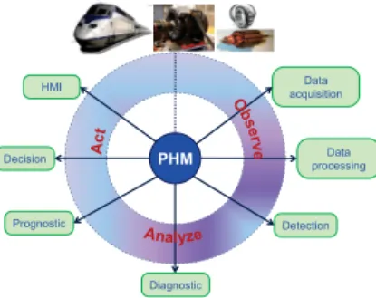
Micro-Electro-Mechanical Systems (MEMS) are micro-systems that integrate mechanical components using elec-tricity as source of energy in order to perform measurement functions and/or operating in structure having micromet-ric dimensions. In the past few years, MEMS devices gained wide-spread acceptance in several industrial seg-ments including aerospace, automotive, medical and even military applications, where they contribute to important functions. The most known applications of MEMS are accelerometers for automotive (airbag) applications, gy-roscopes for mobiles phones, pressure sensors for engine management and micro-mirror arrays for display applica-tions. Nevertheless, the reliability of MEMS is considered as a major obstacle for their development (Medjaher et al. (2014)). They suffer from numerous failure mechanisms which impact their performance, reduce their lifetime, and the availability of systems in which they are used (Huang et al. (2012); Hartzell et al. (2011); Merlijn van Spengen (2003); Li and Jiang (2008)). This analysis shows the need to monitor their behavior, assess their health state and an-ticipate their failures before their occurrence. These tasks can be done by using Prognostics and Health Management (PHM) approaches, and this is the aim of this paper. PHM is the combination of seven layers that collectively enable linking failure mechanisms with life management
⋆ This work has been supported by the R´egion Franche-Comt´e and the ACTION Labex project (contract ANR-11-LABX-0001-01).
PHM Data acquisition Data processing Detection Diagnostic Prognostic Decision HMI
Fig. 1. Prognostics and Health Management cycle. (Fig. 1) (Lebold and Thurston (2001)). It is a discipline that deals with the study of failure mechanisms in order to extend the life cycle of systems and to better manage their health. Within the framework of PHM, prognostics is considered as a core activity for applying a good predictive maintenance. Prognostics is defined by the PHM commu-nity as the estimation of the Remaining Useful Life (RUL) of physical systems based on their current health state and their future operating conditions. Prognostics approaches can be classified into three main approaches (Jardine et al. (2006); Muller et al. (2008); Heng et al. (2009); Peng et al. (2010); Medjaher and Zerhouni (2013)): model-based, data-driven and hybrid prognostics approaches. The model-based approach deals with estimation of the RUL by using mathematical representation to formalize physical understanding of a degrading system. The data-driven approach aims at transforming raw monitoring data
(e.g. temperature, voltage, etc.) into relevant information to build behavior models including the degradation evo-lution, which are then used for RUL estimation. Finally, the hybrid approach combines both previous approaches to achieve more accurate RUL estimates.
This paper proposes a hybrid prognostics approach for MEMS, with a specific application to an electro-thermally actuated MEMS valve. The approach combines two types of models: a nominal model of the MEMS derived by writ-ing its physical laws, and a degradation model obtained from accelerated life tests conducted on several samples of the same reference of MEMS. The generated prognostic model is then used to estimate the RUL of the MEMS. The paper is structured in six sections. After the introduc-tion, Section 2 discusses the implementation of prognostics for MEMS instead of studying their reliability. Section 3 deals with the proposed approach to estimate the RUL of MEMS. The used prognostics tool is presented in Sec-tion 4. SecSec-tion 5 describes the applicaSec-tion of the proposed approach to a MEMS device and presents the obtained results. Finally, Section 6 concludes the paper.
2. TOWARD PROGNOSTICS OF MEMS MEMS devices suffer from various reliability issues. This is confirmed by numerous published works dealing with MEMS reliability. These works concern: 1) testability and characterization of MEMS, 2) identification and under-standing of failure mechanisms, 3) design, fabrication and packaging optimization, 4) accelerated life tests to develop predictive reliability models, and 5) statistical studies of failures on a significant number of samples.
Improving reliability of MEMS devices has several ad-vantages, such as increasing their lifetime and improving their performance. However, reliability still has some limi-tations. It is defined as the ability of a system or a product
to perform its intended function without failure and within specified performance limits for a specified period of time under stated conditions. Thus, according to this definition,
reliability is valid only for given conditions and a period of time. This is the case, for example, for cars which are guaranteed by automobile manufacturers for a period of time in given operating conditions. In this situation, the re-liability is estimated without taking into account the spe-cific utilization of each car (e.g. environment conditions, roads quality, frequency of use, etc.). However, in practice, the lifetime should be different from one car to another depending on how and where it is used. In addition to this, reliability models are generally obtained from statistical data on representative samples. These models, which are generic for all the samples, are not updated during the utilization. This means that, once they are estimated, the model reliability parameters still constant while they should change due to the factors mentioned previously. To cope with the above mentioned limitations, one can use PHM. This activity makes use of past, present, and future operating conditions in order to assess the health state of the system, diagnose its faults, update the degradation models parameters, anticipate failures by estimating the RUL and improve decision making to prolong its lifetime. Prognostics is widely applied in industrial systems ranging
MEMS device
Construction of the nominal behavior model
Accelerated lifetime tests and
measurements Health indicator selection Degradation model definition Online measurements & Particle filter Estimated model parameters Health assessment and prediction Failure threshold ≤ estimation RUL Online phase Offline phase
Fig. 2. Overview of the proposed prognostics approach. from small components (e.g. bearings (Tobon-Mejia et al. (2012)), cutting tools (Javed et al. (2015)), etc.) to com-plete machines (e.g. turbofans (Mosallam et al. (2014)), mechatronic systems (Medjaher and Zerhouni (2013)), etc.). Although its benefits are well proven, there are few published works addressing fault prognostics of MEMS. To fill this gap, a hybrid prognostics approach for MEMS devices is proposed in the next section.
3. PROGNOSTICS APPROACH
The steps of the proposed hybrid prognostics approach are presented in Fig. 2. This approach can be applied on different categories of MEMS at a condition that the following assumptions hold.
• The instrumentation needed to monitor the behavior of MEMS (sensors, camera, etc.) is available. • Sufficient knowledge about the studied MEMS is
available to derive their nominal behavior models and identify their failure mechanisms which may take place during their utilization.
In this work, the approach is applied to an electro-thermally actuated valve MEMS (see Section 5.1). It relies on two phases. The first phase is done offline to build the nominal behavior model of the MEMS, select a relevant physical health indicator and derive the MEMS degra-dation model. The second phase is conducted online and uses the obtained degradation model to predict the MEMS future behavior and calculate its RUL. The steps shown in Fig. 2 can be grouped in three main tasks.
(1) Nominal behavior model construction: it is obtained by writing the corresponding physical laws of the tar-geted MEMS and then validating it experimentally. (2) Degradation model : it is obtained experimentally
through accelerated life tests and it is related to drifts in a selected Health Indicator (HI). This HI is a physical parameter, which can be used to track the degradation of the MEMS.
(3) Prognostics modeling: prognostics is divided into two main stages: learning and prediction. In the learning stage, the prognostics tool combines the available data with the degradation model to learn the behavior of the system and estimate the parameters of its degradation model. This stage lasts until a prediction is required at time tp. Then, in the prediction stage, the prognostics tool propagates the state of the sys-tem and determines at what time the failure threshold (F T ) is reached. Finally, the RUL is calculated as the difference between the failing time Tfand the starting prediction time tp.
In the offline phase, the evolution of the selected HI is approximated by a mathematical model to define the degradation model. In the online phase, the parameters of this model are unknown and need to be estimated as a part of the prognostics process. To do so, the particle filter algorithm is used as a prognostics tool. It allows handling the non-linearities and non-Gaussian noises (Yin and Zhu (2015)), which are some specificities inherent to MEMS.
4. PROGNOSTICS USING PARTICLE FILTERING
4.1 Particle filtering framework
The problem of recursive Bayesian estimation is defined by two equations (Gordon et al. (1993)): the first considers the evolution of the system state {xk, k ∈ N} which is given by: xk = f (xk−1, λk−1) (1) where k is the time step index, f is the transition function from the state xk−1to the next state xkand {λk−1, k ∈ N} is the independent identically distributed process noise sequence. The purpose is to recursively estimate xk from measurements introduced by the second equation and which corresponds to the measurement model {zk, k ∈ N}:
zk= h(xk, µk) (2)
where k is the time step index, h is the measurement function and {µk, k ∈ N} is the independent identically distributed measurement noise sequence.
The aim of the recursive Bayesian estimation problem is to recursively estimate the state of the system by construct-ing the Probability Density Function (PDF) of the state at time k based on all available information, p(xk|z1:k). It is assumed that the initial PDF of the state vector, also called the prior, is available (p(x0|z0) = p(x0)). The PDF p(xk|z1:k), known as the posterior, can be obtained recursively in two main stages: prediction and update.
• Prediction stage: in this stage the state model (Eq. 1) is used to obtain the prior PDF of the state at time k via the Chapman-Kolmogorov equation:
p(xk|z1:k−1) = Z
p(xk|xk−1)p(xk−1|z1:k−1)dxk−1 (3) • Update stage: when a new measurement zk becomes available, one can update the prior PDF via the Bayes rule:
p(xk|z1:k) = p(zk|xk)p(xk|z1:k−1) p(zk|z1:k−1)
(4) This gives the formal solution to the recursive Bayesian estimation problem. Analytic solutions to this problem are available in a restrictive set of cases, including the Kalman filter, which assumes that the state and measurement models are linear and λk and µk are additive Gaussian noise of known variance. When these assumptions are unreasonable, which is the case in many applications, and the equations (Eq. 3) and (Eq. 4) cannot be solved analytically, approximations are necessary. One of the most used approximate solution for this kind of problem is the particle filtering.
The particle filtering solution is a sequential Monte-Carlo method which consists in representing the required poste-rior PDF by a set of particles with associated weights and
computing estimates based on these particles and weights. Different versions of particle filtering are reported in the literature and, for more details, interested readers can refer to the work published by Arulampalam et al. (2002). In this paper, we focus on the Sampling Importance Re-sampling (SIR) particle filer, which is very commonly used in the prognostics field (see An et al. (2013); Saha and Goebel (2011); Jouin et al. (2014)). To explain the steps of the SIR algorithm, let suppose that at time step k = 0, the initial distribution p(x0) is approximated in the form of a set of Ns samples {xi0}Ns
i=1 with associated weights {wi
0= 1 Ns}
Ns
i=1. Then, the following three steps are repeated until the end of the process.
(1) Prediction: a new PDF is obtained by propagating the particles from state k − 1 to state k using the state model (in our case, this corresponds to the degradation model).
(2) Update: when a new measurement is available, the likelihood of the particles p(zk|xi
k) is computed. This probability shows the degree of matching between the prediction and the measurement. Its calculation allows updating the weight of each particle.
(3) Re-sampling: this step appears to avoid a degeneracy of the filter. The basic idea of re-sampling is to elim-inate the particles with small weights and duplicate the particles with large weights. The re-sampling step involves generating a new set of particles {xi∗
k} Ns
i=1 by re-sampling (with replacement) Ns time from an approximate discrete representation of p(xk|z1:k).
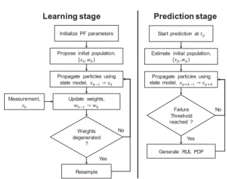
4.2 Particle filter for fault prognostics
In fault prognostics, the SIR particle filter is used in both learning and prediction stages (Fig. 3). In the learning stage, the state of the system and the unknown param-eters of its degradation model are estimated. When a prediction is required, at time tp, the posterior PDF given by {xip, wip}Ns
i=1 is propagated until x
i reaches the failure threshold at Ti
f. The RUL PDF is then given by calculating Ti
f− tp.
Propose initial population, {!", #"}
Resample Propagate particles using
state model, !$%&' !$ Update weights, #$%&' #$ Weights degenerated ? Initialize PF parameters Measurement, ($ Yes No
Estimate initial population, {!), #)}
Generate RUL PDF Propagate particles using state model, !)*$%&' !)* $
Failure Threshold reached ? Start prediction at +) Yes No
Learning stage Prediction stage
Fig. 3. SIR particle filter for fault prognostics (adapted from Saha and Goebel (2011)).
Hot arms Anchorage Anchorage ᶿ Shuttle Direction of movement (a) (b)
Fig. 4. (a) The MEMS valve and (b) schematic view of its actuator.
5. APPLICATION AND RESULTS
5.1 The MEMS and its nominal behavior model
The targeted device consists of an electro-thermally ac-tuated MEMS valve of DunAn Microstaq, Inc. (DMQ) company (Fig. 4(a)). It is designed to control flow rates or pressure with high precision at ultra-fast time response (<< 100 ms). It is currently being used in a number of applications in air conditioning and refrigeration, hy-draulic control and air pressure control. The valve is com-posed of three silicon layers. The center layer is a movable membrane, the top layer is for electrical connections and the bottom layer is for the three fluid connections ports: common port, normally closed and normally open. The maximum actuation voltage of the valve is 12 V .
The actuator used inside the targeted MEMS is an electro-thermal actuator. This actuator, presented in Fig. 4(b), is composed of hot arms inclined to the horizontal axis by an angle θ and clamped to the substrate and the freestanding central shuttle. When a voltage difference is applied across the anchor sites, a heat is generated along the beams due to ohmic dissipation. The hot arms expand to push ahead symmetrically on the central part of the actuator (the shuttle). This part moves in the direction shown in Fig. 4(b). The shuttle is connected to the membrane and its movement allows moving the membrane to open or close the fluid ports.
The physical modeling of the MEMS behavior leads to a first order model. This model,given by equation 5, is confirmed by the experimental results described in the next subsection.
X(p) U (p) =
K
1 + τ p (5)
In this equation, X is the output of the system (displace-ment of the actuator), U is the input (voltage), K is the static gain and τ is the time constant.
5.2 Experimental setup and tests
In order to validate the nominal behavior model and per-form accelerated lifetime tests to generate the degradation model of the targeted MEMS, we designed and built an experimental platform (Fig. 5). This platform is composed of two ARDUINO devices, two voltage suppliers, supports for the camera and the MEMS, a light source for the camera allowing to see the movement of the membrane inside the MEMS, an air inlet, a pressure regulator, an NI card and a computer for data acquisition. Four MEMS are cycled at each experimental campaign. Each MEMS
Voltage suppliers Light source Arduino NI card MEMS Camera Anti-vibration table
Fig. 5. Overview of the experimental platform.
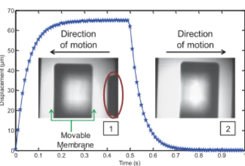
0 0.1 0.2 0.3 0.4 0.5 0.6 0.7 0.8 0.9 1 0 10 20 30 40 50 60 70 Time (s) D isp la ce m e n t (µ m ) 1 2 Direction of motion Movable Membrane Direction of motion
Fig. 6. Time response of the MEMS valve. At 8 V , the membrane moves (image 1) to create an output or an input of the air (circled part). At 0 V , the membrane returns to its initial position (image 2).
is fixed on a support specially designed. To minimize the mechanical vibration, the experimental platform is placed on an anti-vibration table.
During the accelerated lifetime tests, the supply voltage is set to 8 V . This value is not too high to not bring up prematurely degradation and not too low to obtain enough displacement. The time response of the MEMS is obtained by using the images taking by the camera and a Matlab image-processing algorithm. Fig. 6 shows an example of an obtained time response of one MEMS valve supplied by a periodic square signal of 8 V magnitude and 1 Hz frequency. This time response is typical of a first order system. By using the Matlab system identification toolbox, the transfer function can be obtained and all the system parameters can be easily identified. The transfer function corresponding to the time response presented in Fig. 6 is given in equation 6 and the identified parameters are given in table 1.
X(p) U (p) =
8.02
1 + 0.052p (6)
Table 1. Identified parameters.
Parameter Symbol Value Unit
Displacement D 65 µm Current I 0.5 A Static gain K 8.02 µm/V Time constant τ 0.052 s Stiffness ks 2.7 × 10− 2 N/m Friction coefficient f 1.4 × 10⁻³ N s/m
Accelerated lifetime tests consist in cycling continuously four MEMS valves (Fig. 5). They are supplied by a periodic square signal of 8 V magnitude and 1 Hz frequency. The measurements acquisition is the same for all the tested MEMS. For each one of them the following steps are applied: 1) adjust the MEMS below the camera by using a 3D positioner until having a very clear image, 2) get the time response by using a Matlab image-processing algorithm, 3) identify the parameters of the system by using the Matlab system identification toolbox, and 4) store the results in different files in a dedicated computer for later use. Note that, the operating conditions and load were kept constant during the cycling tests.
5.3 Degradation model
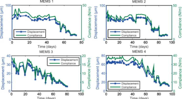
To get the degradation model of the MEMS, the accel-erated lifetime tests remained running for approximately three months, during which the MEMS valves were con-tinuously cycled. During this period, measurements were collected every day. The decrease in the magnitude of the displacement is related to the degradation in the tested MEMS valves (Fig. 7). Among the defined parameters, the compliance 1/ks(inverse of the stiffness) has the same evolution in time as the displacement (Fig. 7). Therefore, the compliance is selected as the physical HI, which can be used to track the degradation of the MEMS valves. The projection of this HI can be exploited to predict the future behavior of each MEMS valve and calculate its RUL. Prior to curve fitting task to derive the degradation model, the raw experimental data are smoothed by applying a
rloess filter to remove the different peaks and extract a
monotonic trend (Fig. 8). Basically, rloess is a robust local regression filter that allocates lower weight to outliers. By using the curve fitting method, the evolution of the HI is approximated by a double exponential model, which represents the degradation model of the MEMS valves:
HI(t) = a.eb.t+ c.ed.t (7) The four tested MEMS valves have the same shape of the degradation model (Eq. 7), but with different values of the parameters (a, b, c and d). Thus, this model is set as a generic degradation model for the studied MEMS valve.
5.4 Prognostics results
The RUL estimation of each MEMS requires a definition of a corresponding Fault Threshold (F T ). In this case study, the F T corresponds to the point at which the HI value decreases by 60%. Obviously, this value can be changed depending on the desired performance of the MEMS. As explained in Section 3, prognostics is divided into two stages: learning and prediction. During the learning stage, the state of the MEMS (PDF of the HI) at time step k is estimated using the degradation model and the state at time step k − 1. The parameters of the state model are consequently adjusted. This process lasts until a prediction is required at tp. At this time, the estimated PDF of the HI is propagated until it reaches the F T at Tf. The duration between Tf and the starting point of prediction tpgives the PDF of the RUL.
0 20 40 60 80 0 100 Displacement (µ m) Time (days) MEMS 1 0 20 40 60 800 50 Compliance (N/m) 0 20 40 60 80 100 0 100 Displacement (µ m) Time (days) MEMS 2 0 20 40 60 80 1000 50 Compliance (N/m) 0 20 40 60 80 100 0 10 20 30 40 Displacement (µ m) Time (days) MEMS 3 0 20 40 60 80 1000 5 10 15 20 Compliance (N/m) 0 20 40 60 80 100 0 20 40 60 80 Displacement (µ m) Time (days) MEMS 4 0 20 40 60 80 1000 10 20 30 40 Compliance (N/m) Displacement Compliance Displacement Compliance Displacement Compliance Displacement Compliance
Fig. 7. Displacement and compliance as functions of time.
0 20 40 60 80 0 10 20 30 40 Time (days) Health indicator MEMS 1 Raw data Filtered data 0 20 40 60 80 100 0 10 20 30 40 Time (days) Health indicator MEMS 2 Raw data Filtered data 0 20 40 60 80 0 5 10 15 20 Time (days) Health indicator MEMS 3 Raw data Filtered data 0 20 40 60 80 100 0 10 20 30 40 Time (days) Health indicator MEMS 4 Raw data Filtered data
Fig. 8. Filtering raw experimental data using ”rloess”.
10 20 30 40 50 60 70 80 90 10 15 20 25 30 35 40 Time (days) He a lth in d ica to r
Current health indicator Estimated health indicator Threshold
Lower bound of the confidence interval upper bound of the confidence interval
Real RUL Estimated RUL !" Learning Prediction Threshold
(a) RUL estimation at 60 days.
35 40 45 50 55 60 65 70 75 80 85 0 10 20 30 40 50 Time (days) RUL Real RUL Estimated RUL 95% prediction interval
(b) RUL estimation at frequent intervals. Fig. 9. Prognostics results.
An example of RUL estimation at 60 days is given in Fig. 9(a). The estimated health indicator is represented with a confidence interval of 95%. The current HI is also drawn to show the difference. The estimated RUL corresponds to the median of the RUL PDF. The median RUL is chosen rather than the mean RUL since it gives early estimates and has better accuracy when more data
are available. Note that, in PHM context, it is better to have early estimates rather than late RUL to avoid failures. In order to demonstrate the online estimation of the RUL, the prediction is initiated at regular intervals. Fig. 9(b) shows the estimated RUL at regular intervals compared to the real one. One can clearly see that the accuracy of the RUL estimates increases with time, as more data are available. Furthermore, the estimated RUL still in the 95% prediction interval at different time steps. These obtained results demonstrate the accuracy and the significance of the proposed prognostics approach.
6. CONCLUSION
In this paper, a hybrid prognostics approach is proposed. First, before presenting the approach, the necessity of implementing PHM for MEMS devices instead of simply studying their reliability is discussed. After that, a brief presentation of the particle filter algorithm is given. The proposed approach is then applied to an electro-thermally actuated MEMS valve. For this purpose, an experimental platform is designed to validate the obtained nominal behavior model of the targeted MEMS, perform accelerated lifetime tests and derive its degradation model. Once the degradation model is obtained, the SIR particle filter is used to perform online prognostics. This tool al-lowed to estimate the degradation model parameters, pre-dict the future behavior of the MEMS valve and calculate its RUL. The obtained results show the significance of the proposed prognostics approach.
As a future work, this approach will be implemented on a real application: a centimeter contact-less distributed MEMS-based conveying surface. This application, con-ducted in our laboratory, is dedicated for distributed post-prognostics decision making and aims at optimizing the utilization of the conveying surface and maintaining a good performance as long as possible.
REFERENCES
An, D., Choi, J.H., and Kim, N.H. (2013). Prognostics 101: A tutorial for particle filter-based prognostics algorithm using matlab. Reliability Engineering & System Safety, 115, 161–169.
Arulampalam, M.S., Maskell, S., Gordon, N., and Clapp, T. (2002). A tutorial on particle filters for online nonlinear/non-gaussian bayesian tracking. Signal
Pro-cessing, IEEE Transactions on, 50(2), 174–188.
Gordon, N.J., Salmond, D.J., and Smith, A.F. (1993). Novel approach to nonlinear/non-gaussian bayesian state estimation. In Radar and Signal Processing, IEE
Proceedings F, volume 140, 107–113. IET.
Hartzell, A.L., Da Silva, M.G., and Shea, H.R. (2011).
MEMS reliability. EPFL-BOOK-154162. Springer.
Heng, A., Zhang, S., Tan, A.C., and Mathew, J. (2009). Rotating machinery prognostics: state of the art, chal-lenges and opportunities. Mechanical Systems and
Sig-nal Processing, 23(3), 724–739.
Huang, Y., Vasan, A.S.S., Doraiswami, R., Osterman, M., and Pecht, M. (2012). MEMS reliability review. Device
and Materials Reliability, IEEE Transactions on, 12,
482–493.
Jardine, A.K., Lin, D., and Banjevic, D. (2006). A review on machinery diagnostics and prognostics implementing condition-based maintenance. Mechanical systems and
signal processing, 20(7), 1483–1510.
Javed, K., Gouriveau, R., Zerhouni, N., and Nectoux, P. (2015). Enabling health monitoring approach based on vibration data for accurate prognostics. Industrial
Electronics, IEEE Transactions on, 62(1), 647–656.
Jouin, M., Gouriveau, R., Hissel, D., P´era, M.C., and Zerhouni, N. (2014). Prognostics of PEM fuel cell in a particle filtering framework. International Journal of
Hydrogen Energy, 39(1), 481–494.
Lebold, M. and Thurston, M. (2001). Open standards for condition-based maintenance and prognostic systems. In Maintenance and Reliability Conference (MARCON), 6–9. May.
Li, Y. and Jiang, Z. (2008). An overview of reliability and failure mode analysis of microelectromechanical systems (MEMS). In Handbook of performability engineering, 953–966.
Medjaher, K., Skima, H., and Zerhouni, N. (2014). Condi-tion assessment and fault prognostics of microelectrome-chanical systems. Microelectronics Reliability, 54, 143– 151.
Medjaher, K. and Zerhouni, N. (2013). Hybrid prognostic method applied to mechatronic systems. The
Interna-tional Journal of Advanced Manufacturing Technology,
69(1-4), 823–834.
Merlijn van Spengen, W. (2003). MEMS reliability from a failure mechanisms perspective. Microelectronics
Re-liability, 43, 1049–1060.
Mosallam, A., Medjaher, K., and Zerhouni, N. (2014). Data-driven prognostic method based on bayesian ap-proaches for direct remaining useful life prediction.
Journal of Intelligent Manufacturing, 1–12.
Muller, A., Suhner, M.C., and Iung, B. (2008). Formalisa-tion of a new prognosis model for supporting proactive maintenance implementation on industrial system.
Re-liability Engineering & System Safety, 93(2), 234 – 253.
Peng, Y., Dong, M., and Zuo, M.J. (2010). Current status of machine prognostics in condition-based maintenance: a review. The International Journal of Advanced
Man-ufacturing Technology, 50(1-4), 297–313.
Saha, B. and Goebel, K. (2011). Model adaptation for prognostics in a particle filtering framework.
Interna-tional Journal of Prognostics and Health Management Volume 2 (color), 61.
Tobon-Mejia, D.A., Medjaher, K., Zerhouni, N., and Tripot, G. (2012). A data-driven failure prognostics method based on mixture of gaussians hidden markov models. Reliability, IEEE Transactions on, 61(2), 491– 503.
Yin, S. and Zhu, X. (2015). Intelligent particle filter and its application on fault detection of nonlinear system.
Industrial Electronics, IEEE Transactions on, 62(6),