OATAO is an open access repository that collects the work of Toulouse
researchers and makes it freely available over the web where possible
Any correspondence concerning this service should be sent
to the repository administrator:
[email protected]
This is a
publisher’s version published in:
https://oatao.univ-toulouse.fr/27538
To cite this version:
A study on the relationship between upstream and
downstream conditions in swirling two-phase flow / Benjamin
Sahovic, Hanane Atmani, Philipp Wiedemann, Eckhard
Schleicher, Dominique Legendre, Éric Climent, Rémi
Zamansky, Annaig Pedrono, Uwe Hampel. Flow
Measurement and Instrumentation, 2020, 74, 101767
Official URL:
https://doi.org/10.1016/j.flowmeasinst.2020.101767
Open Archive Toulouse Archive Ouverte
Flow Measurement and Instrumentation 74 (2020) 101767
Available online 6 June 2020
0955-5986/© 2020 The Authors. Published by Elsevier Ltd. This is an open access article under the CC BY license (http://creativecommons.org/licenses/by/4.0/).
A study on the relationship between upstream and downstream conditions
in swirling two-phase flow
B. Sahovic
a,*, H. Atmani
b, P. Wiedemann
a, E. Schleicher
a, D. Legendre
b, E. Climent
b,
R. Zamanski
b, A. Pedrono
b, U. Hampel
a,caHelmholtz-Zentrum Dresden-Rossendorf, Institute of Fluid Dynamics, Bautzner Landstraße 400, 01328, Dresden, Germany
bInstitut National Polytechnique de Toulouse, Institut de M�ecanique des Fluides de Toulouse, All�ee Emile Monso 6, 31029, Toulouse, Cedex 4, France cTechnische Universit€at Dresden, Chair of Imaging Techniques in Energy and Process Engineering, 01062, Dresden, Germany
A R T I C L E I N F O
Keywords:
Gas/liquid flow Inline fluid separation Swirling element Wire-mesh sensor Digital image processing High-speed camera
A B S T R A C T
Inline fluid separation is a concept, which is used in the oil and gas industry. Inline fluid separators typically have a static design and hence changing inlet conditions lead to less efficient phase separation. For introducing flow control into such a device, additional information is needed about the relationship of upstream and downstream conditions. This paper introduces a study on this relationship for gas/liquid two-phase flow. The downstream gas core development was analyzed for horizontal device installation in dependence of the inlet gas and liquid flow rates. A wire-mesh sensor was used for determining two-phase flow parameters upstream and a high-speed video camera to obtain core parameters downstream the swirling device. For higher accuracy of the calculated void fraction, a novel method for wire-mesh sensor data analysis has been implemented. Experimental results have shown that void fraction data of the wire-mesh sensor can be used to predict the downstream behavior for a majority of the investigated cases. Additionally, the upstream flow pattern has an impact on the stability of the gas core downstream which was determined by means of experimental data analysis.
1. Introduction
Fluid separation is a typical task in many fluids processing applica-tions. One prominent example is oil extraction, for which separation of oil and water is one of the processing stages [1]. The efficiency of the entire process is generally poor and added chemicals for treatment are a big problem for the environment [2]. An undesirable outcome is oil-contaminated water. For the average lifetime of a reservoir, it is estimated that 2.6 to 4 barrels of water are produced for each barrel of oil [3]. Moreover, fluid separation is an important operation not only in the oil and gas industry. Nuclear power plants also use such techniques for removal of radiolysis gases from water in a nuclear fission reactor [4]. In addition, in the chemical industry fluid separation devices are very common.
There are different mechanical approaches to separate fluids. Hydro- cyclones separate a dispersed phase from a continuous one by redi-recting flow in order to apply centrifugal forces that create a pressure field to separate the phases by inertia and redirecting them to different outlets. Gravitational separators are large vessels in which the mixtures
of oil, water, gas, and also sand, are separated slowly by gravitation over a longer time span. The third approach is inline-fluid separation. The central part of such a unit is a swirl element (Fig. 1) which sets the incoming stream into strong rotational motion. Hence, inline fluid sep-aration uses centrifugal force with much higher strength than gravita-tional force. The centered less dense fluid is extracted via a pick-up tube.
The advantage of inline fluid separation over the other methods is easy installation and low cost. A major downside is low separation ef-ficiency in case of varying inlet flow conditions. The efef-ficiency mostly depends on the stability of the core of the swirling lighter fluid. At high velocities, increased shear will lead to fluid mixing and turn the unit into a mixer [5]. At low velocity, however, centrifugal forces may be not strong enough to sustain the core. Due to the high cost and troublesome installation of conventional (gravitational) subsea separators, present and future industry standards are in need of a fully controlled inline fluid separator. To develop such control systems, further knowledge is required to understand the behavior of the low-density fluid core at different inlet flow conditions. As the centrifugal force generated inside the separator has a bigger impact on denser fluids in a multiphase flow, * Corresponding author.
E-mail addresses: [email protected], [email protected] (B. Sahovic).
Contents lists available at ScienceDirect
Flow Measurement and Instrumentation
journal homepage: http://www.elsevier.com/locate/flowmeasinst
https://doi.org/10.1016/j.flowmeasinst.2020.101767
the separation of air/water mixture is easier than oil/water due to larger difference in density between the mixed fluids.
An exemplary system design is shown in Fig. 1. A pick-up tube placed inside the pipe in the downstream section extracts the less dense fluid from the centered rotating core. The incoming fluid passes through the blades of the fixed swirl element, creating a vortex shaped gas core. Instability and temporal fluctuation of the core are characterized by a change in diameter and waviness, that is, fluctuation around the mean diameter and the standard deviation from the average core diameter. An ideal core may be one that has a geometry close to an ideal cylinder with a diameter equal to the one of the pick-up tube. Then, separation effi-ciency would be continuously optimal. However, in the application the core diameter fluctuates with the incoming mixture flow rate and composition. Hence, static separator designs, e.g. with a fixed pick-up tube, have separation deficiencies because of that dynamics. Accord-ing to experiments performed with an inline fluid separator in Refs. [4], valves mounted on tubes of separated fluids change the behavior of gas core downstream. In order to control these valves, imaging sensors may be placed upstream and downstream of the swirl providing the required control parameters. Such sensors can be e. g. electrical tomography sensors [6], wire-mesh sensors (WMS) [7] or simpler sensors, like ul-trasound sensors or optical probes. Objective of this study was to determine the relationship between upstream flow conditions and downstream gas core behavior in an inline fluid separator.
2. Experimental setup and data processing 2.1. Test facility and experiments
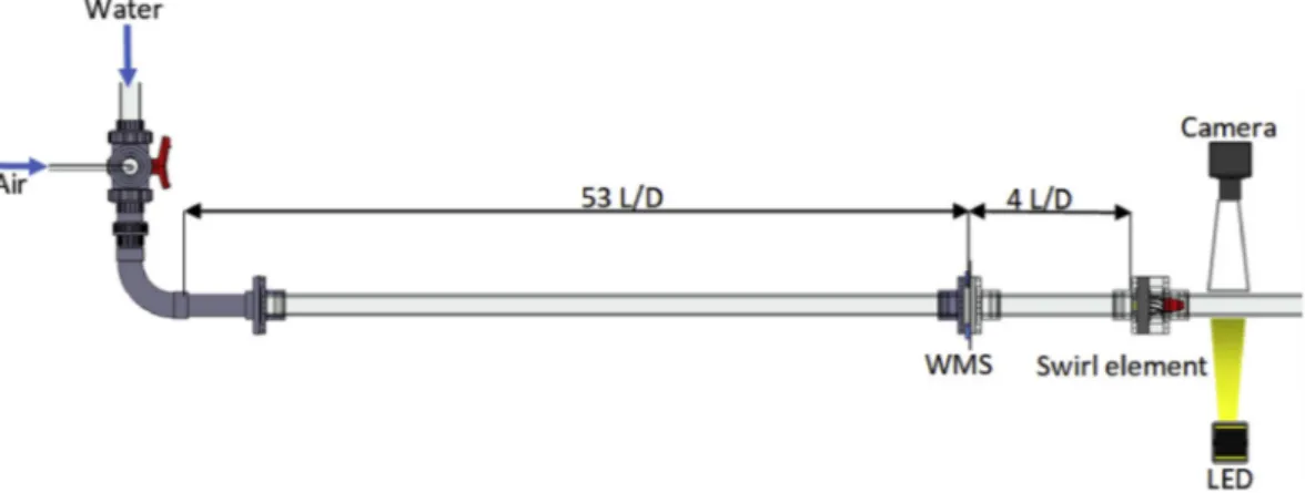
Experiments were performed on an existing but slightly modified gas/liquid two-phase flow loop installation (Wiedemann [8]) at Helmholtz-Zentrum Dresden-Rossendorf (HZDR). The horizontal test section consists of acrylic pipes of 50 mm inner diameter. A wire-mesh sensor is mounted at 53 L/D downstream the last elbow in order mea-sure a sufficiently developed two-phase flow. The swirl element is placed after further 4 L/D. A high-speed camera was installed 2 L/D down-stream the swirl element tail in order to record the gas core dynamics. Transparent pipes were used for ease of camera recording and visual observation. The experimental setup is depicted in Fig. 2.
Experiments were performed for different gas and liquid flow rates
which are further expressed in terms of superficial velocities Jsg and Jsl,
respectively. The volumetric flow rate of the water _Vl was adjusted by
speed control of the pump and measured by magnetic-inductive flow meters. The superficial velocity is then obtained from
Jsl¼ _
Vl
A (1)
where A denotes the cross-sectional area of the pipe. Since air is a compressible fluid, its superficial velocity was adjusted by means of mass flow controllers while accounting for temperature Tg and local
gauge pressure prel: Jsg¼ _ Vg;S A ⋅ Tg TS ⋅ pS ðpambþprelÞ (2)
Here, _Vg;S denotes the volumetric gas flow rate at standard conditions
pS and TS, and pamb is the ambient pressure.
Experiments were performed in an operating range of practical in-terest, i.e. close to industrial scenarios, as can be seen from Fig. 3, where the experimental points are plotted into the flow map of Mandhane [9]. The dashed points were found unstable and therefore not included in the further analysis. The onset of stable gas core formation was identified at a superficial liquid velocity of approximately 0.6 m/s. Further limita-tions of the operation range were given by unstable gas injection at low gas flow rates as well as pump and pipe characteristics at maximum liquid flow rates.
The experiments were performed in such a way, that the liquid flow rate was kept constant and the superficial gas velocity was increased in certain steps. After one run, the liquid flow rate was increased. The sampling of the matrix was rather regular in logarithmic scale. There-fore, we may effectively compare between experiments at constant liquid flow rate and experiments at constant gas flow rate in the analyses in section 3.
2.2. Camera operation and image processing
The high-speed camera records the flow downstream the swirl, that is, the gas core. Images were taken with a frequency of 250 frames per second for a total time of 12 s per experiment giving 3000 frames per experimental point in total. A flat LED light source was mounted on the
Fig. 1. Principle of inline fluid separation, here for gas/liquid separation.
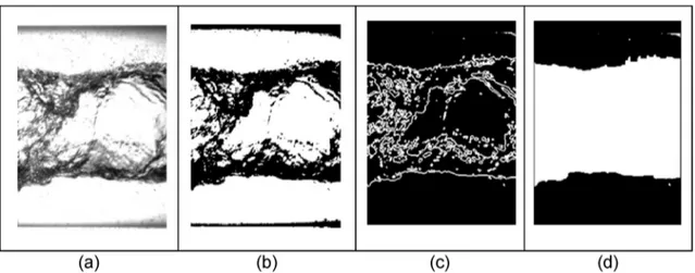
opposite side of the camera, illuminating the entire section. Care was given to avoid reflections in the wall of the pipe. In this configuration, the gas core appears as a semitransparent shadow in the images. Due to the optimized video setup, no additional techniques for image pre- processing like contrast adjustment or brightness modification had to be applied to the images. Post processing of the images was done using MATLAB® and is schematically shown in Fig. 4.
Fig. 4a) shows the unprocessed gas core in the transparent pipe. The boundaries are recognizable from light refraction, that is, a change of light wave direction when it hits a surface boundary between air and water. Segmentation is used to manipulate pixel intensities to create objects of interest from the captured photos. The first step is to separate regions of interest from the background.
The implemented algorithm performs a pixel transformation in a loop by binarizing each pixel from the camera images fðxi;yjÞwith a threshold value T to get a new binary image gðxi;yjÞ, according to
g xi;yj � ¼ � 1 if f xi;yj � > T 0 otherwise (3)
Otsu’s method [10] has been used for obtaining the value T, which is the value that minimizes the intraclass variance of the dark and bright pixels intensity. The resulting images are in binary format (Fig. 4b). The
binary image is further processed with an edge operator that finds the borders from the magnitude of their gradient, given by
rg ¼ � Gx Gy � ¼ 2 6 6 6 4 ∂g ∂x ∂g ∂y 3 7 7 7 5 (4) mag ðrgÞ ¼ ffiffiffiffiffiffiffiffiffiffiffiffiffiffiffiffiffi G2 xþG2y q : (5)
If the magnitude of the gradient in specific location is greater or equal to one, it means an edge is detected.
Fig. 4c shows an image with region boundaries represented as edges. Numerous interfacial structures apparently detected in the bulk region of the flow are not of interest. In reality, they stem from the light refraction at waves of the gas/liquid interface and not from the central gas core region. Adding a single column of pixels at the right and left to the image with upper and lower gas/liquid boundaries (Fig. 4c), we get a closed gas region. The binarized gas core is obtained by performing a flood-filling operation on background pixels in detected closed regions [11]. The result is shown in Fig. 4d. The average diameter of the gas core in a frame is obtained by dividing the sum of all pixels inside the core by
Fig. 3. Experimental points in the flow map of Mandhane [9] (solid: stable core formation, dashed: unstable core or even no gas core formation).
Fig. 4. Illustration of the camera image processing steps. a) Original image, b) Binarized image c) Extracted boundaries after application of an edge operator, d)
the width of the frame. The average core diameter in pixels per exper-imental point is then calculated by averaging the diameters from all frames. Previously mentioned steps used for image segmentation and getting the gas core geometry in pixels were also applied for segmenting the pipe and expressing pipes height and width in pixels. We have calculated the length of a single pixel and expressed it in millimeters by comparing the height of the pipe in pixels and the outer diameter in millimeters. Using pixel length, we have transformed the average gas-core diameter into millimeters. For hydrodynamic analysis, we computed the diameter of the gas core, its standard deviation and the frequency of its fluctuations over time from the images. The standard deviation was calculated as
SD ¼ ffiffiffiffiffiffiffiffiffiffiffiffiffiffiffiffiffiffiffiffiffiffiffiffiffiffiffiffiffi PN i¼1ðDi μÞ2 N s (6) with Di being the average diameter of the single frame i, μ being the
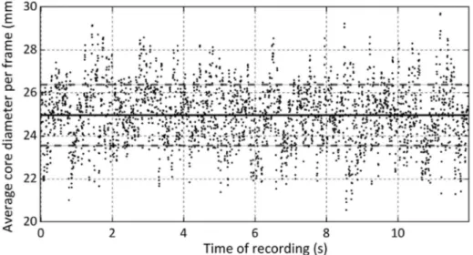
calculated mean value for one experimental point and N the number of frames per measurement. Furthermore, we calculated the frequency of core fluctuations, that is, the number of times the diameter of the gas core shrinks below its mean value and expands beyond it in 1 s. Fig. 5 shows exemplarily the fluctuations around the mean value for a single experimental point.
3. Wire-mesh sensor 3.1. WMS description
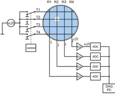
For upstream data acquisition processing, we used a conductivity wire-mesh sensor (Fig. 6). A wire-mesh sensor consists of two planes of parallel wires in the pipe cross-section. The two planes are separated by a small axial distance and arranged so that they form an angle of 90�to each other. In the one transmitter plane, wires are sequentially activated with a square wave excitation voltage signal while at the receiver wires in the other plane transmitted electrical currents are simultaneously sampled. This way the electrical conductance in the crossing-points is obtained with high speed of up to 10,000 frames per second. It should be noted that two types of wire-mesh sensors exist which work on measuring different electrical properties of fluids. Capacitance type [7], which obtains local instantaneous electrical permittivity values, and conductivity type [12], which obtains the local instantaneous conduc-tance, respectively resistance values. In our study, we used the latter. The wire-mesh sensor in our experiments is made of 16 by 16 electrode grid. Spatial and axial resolution are 3.125 mm and axial 1 mm, respectively. Information contained in the current produced from the
crossing points of the transmitter and receiver wires is transformed into voltage signal by a transimpedance amplifier stage. Voltages signals are sampled by analog-to-digital converters (ADC). Digitized signals are further processed via a personal computer.
3.2. WMS data analysis
In order to calculate the local instantaneous void fraction values εi:j:n
of a crossing with indices i; j and the frame number n from the measured signals Umeas
i;j;n usually a first order approximation is used. Here, a linear
relation between measured signal and the local gas holdup within the corresponding area of the virtual wire crossing is assumed, cf [13].:
εi:j:n¼1 Umeas i;j;n UW i;j (7) Here, UW
i;j denotes the local signal for a water only measurement, which is usually the time averaged sensor signal of the full water cali-bration measurement. In our study, we were interested in the cross- sectionally averaged void fraction given by
εn¼ X i X j ai;j⋅εi;j;n (8)
with εi;j;n denoting the measured void fraction in the crossing i;j. Variable ai;j is a weight coefficient that denotes the share of a crossing point with the cross-section [14]. Effectively ai;j accounts for lower share of
crossing points at the pipe boundary. The total mean void fraction, with
N number of frames, is calculated as
ε¼1
N⋅
XN n¼1
εn (9)
As mentioned above the calibration file, used to calculate instanta-neous void fractions having mesh point values UW
i;j, is usually obtained by averaging those values in a gas free flow with only water flowing through the pipe. The downsize of this calibration method is to have conductance values of mesh points in a pure water flow taken before the actual measurement. This leads to possible inaccurate voltage signal representation of pure water flow due to changes in conductance or temperature values that might occur over time e. g. due to heat up by the pump in a closed uncooled loop. Thus, another calibration method is using the pointwise histogram of one entire measurement [14]. Except for stratified and annular flow, it can be assumed that each single crossing point will be in contact with the liquid phase several times during one measurement. Plotting a histogram of all measured values
Umeas
i;j;n for one crossing point i; j will show two peaks in case of two-phase flow: the gas peak at zero and a water peak. This water peak is further used as the water calibration value. This method has the advantages of overcoming the temperature drift problem. Moreover, it compensates for any other disturbances as local impurities on the wires. From the histogram it is clear that there can be also slightly higher values than the peak value. According to eq. (7) higher values than the calibration values would lead to negative void fraction values. According to the established practice [12] the mesh points with negative instantaneous local void fractions are cut off and replaced with zeros. Appearance of higher conductance value is caused by temporarily increase in electrical potential field around a mesh point in an air and water mixture flow. One case of such behavior is registered by mesh points which are on the border and nearby of passing bubbles [15]. The second case is higher measured conductance values in the bulk fluid in case of stratification or larger plug bubbles. This effect can be explained by non-ideal electronics circuit conditions. An ideal trans-impedance amplifier has a resistance of zero on its negative input. However, since the wires always have a small axial resistance this value is not ideal zero. Even if deionized water has a low conductivity this wire resistance leads to a voltage divider and a small portion of current flows towards the grounded transmitter wires instead towards the amplifier input. Thus, the measured signal in a completely liquid filled pipe is smaller than e. g. in a pipe with 25% water at the bottom for the same crossing.
Therefore, receiver wires may also measure higher conductance of a mesh point being fully occupied by water, in mixture of air water flow, compared to the same mesh point condition in a pure water flow, even in regions far from the gas liquid interface. This effect is stronger for long and thin wires, small grid spacing and higher liquid conductivity values. It was shown in Ref. [15] that the linear method overestimates the averaged void fractions, especially in case of bubble flows. The analyses in Ref. [15] were based on the Maxwell method for the calculation of the local instantaneous void fraction
εi:j:n¼ 1 gi;j;n 1 þ1 2⋅ gi;j;n ;gi;j;n¼ Umeas i;j;n UW i;j (10) and have shown that higher accuracy in average void fraction calcula-tion was obtained in comparison to the linear relacalcula-tionship, i.e. equacalcula-tion (7). The method of [15] does not cut off negative void fractions. The results were obtained by performing experiments and numerical simu-lations in the bubbly flow regime.
In order to compare the two different methods, the Maxwell model has been implemented in MATLAB® to perform each step of mean void
fraction calculation including the formation of the histogram calibration file. In contrast to Ref. [15], negative values are kept only if they occur at the liquid gas interface. Negative values in the bulk region are set to zero otherwise the algorithm has derived negative results for the cross-sectional averaged void fraction for particular cases. In contrast to equation (8), the cross-sectionally averaged void fraction is thus ob-tained through εn¼ X i X j
ai;j⋅ bi;j;n⋅εi;j;n (11)
where bi;j;n are the elements of the bulk removal mask. A detailed
description of the calculation of the bulk removal mask is presented in the next section.
3.3. Detection and removal of negative void fractions in bulk regions
To distinguish the noise from the actual signal, a noise filter is used in the WMS framework [14]. Such noisy signal is considered if a mesh point registers a threshold value of 10% local gas hold up or less in pure water without connection to any larger bubble structure. In case of local void fraction having a value above the threshold, the filter will inspect the surrounding points. If all of the surrounding points have values below threshold than the analyzed mesh point is considered to be in water and its value is set to zero. If at least one of the eight surrounding points has a value higher than the threshold, it is assumed the mesh point is located on an edge of a bubble. Negative values surrounding a bubble should be included in the void fraction calculation.
A newly built filter removes the negative void fractions in the bulk region from all negative values, thus leaving only the ones at the boarder to larger gas pockets e. g. surrounding bubbles. Each step in the filter creates a matrix in the shape of the initial one taken from the wire-mesh sensor (Fig. 7a).
The steps for removal of negative values in the bulk region starts by finding all negative values in a frame (Fig. 7b). Let En denote the matrix of local instantaneous void fractions values (eq. (10)) and n the number of the frame. Then we calculate the negative value matrix Nn via the Hadamard product
Nn¼ 1 2⋅ sgn
2ðEnÞ∘ðJ sgnðE
nÞÞ (12)
with the all-one matrix J. All detected negative values are transformed to one and the rest to zero using equation (12). The function denoted as
sgn detects the algebraic sign of each matrix element. Results of the sgn
function using elements of matrix E is described below
sgnεi:j:n � ¼ 8 < : 1;εi;j;n <0 0;εi;j;n ¼0 1;εi;j;n >0 (13) Next stage is the comparison of all points in E to a user defined void fraction threshold to identify bubbles. Points that are above threshold value are replaced with a logical one indicating a connection to a bubble and the rest with a zero value. Outcome of such comparison is stored in the bubble identification matrix D. All elements in matrix T are equal to the threshold value.
D ¼ 1 2⋅ sgn
2ðT EnÞ∘ðJ sgnðT EnÞÞ (14)
At this stage it is not important whether the valid points are on the edge or positioned closer to the center of a bubble. Several of these points can form a bigger bubble if they are in contact to each other. The elements surrounding these bubbles are considered as borders. To assign a value of one to the borders and the rest as zero, we first start by convoluting a matrix K over the bubble identification matrix D. The convolution will enhance the values of located bubbles and their sur-roundings. Therefore, the matrix K used as the kernel for the 2D
convolution has a size of m ¼ 3 by n ¼ 3 with all variables equal to one. In a 2D convolution with a kernel size 3 and a stride number of one (distance between two consecutive positions of the kernel), the output will shrink in size by two compared to the size of the input. To prevent this a zero-padding operation is performed on D (Fig. 8).
The padded matrix P has the dimension p ¼ i þ 2; q ¼ j þ 2. This step can be avoided if the software used for calculating the 2D convo-lution, labels the values outside the input frame as zero. The mathe-matical formulation of 2D convolution with input elements pp; q from
matrix P and kernel elements ka;b is given by
ci;j¼ X∞ a¼ ∞ X∞ b¼ ∞ pi a;i b⋅ka;b (15)
A computational problem occurs with the above equation when the code tries to access elements outside of the frame matrix. To avoid putting additional constraints and to reduce the computation time, the convolution in our case can be written as
ci;j¼ Xm a¼1 Xn b¼1 piþa 1;jþb 1⋅ ka;b;C ¼ 2 4c1; 1⋮ ⋯ c⋱ 1; j⋮ ci; 1 ⋯ ci; j 3 5 (16)
Values of the bubbles and their borders are only important if they differ from zero. Therefore, the values in matrix F are binarized ac-cording to (17)
F ¼1
2⋅ sgnðCÞ∘ðJ þ sgnðCÞÞ (17)
A logical one is produced if ci;j is greater than zero. Variables equal to zero are unchanged. The border matrix G is calculated by subtracting the convolution matrix with the bubble identification matrix to have only border values (19)
G ¼ F D: (18)
Positions of physically plausible negative values at the boundary of a gas volume are obtained with a point by point multiplication between matrix G and the initial negative value matrix N
H ¼ G∘N: (19)
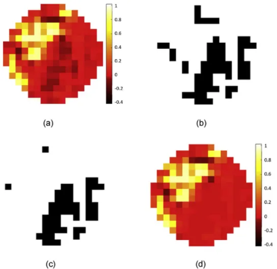
Fig. 7. Process of removing negative bulk values from WMS processed data of a frame in point 66. a) Cross sectional view of calculated local instantaneous void
fraction with color bar indicating void fraction, b) Detected negative values (dark pixels are zero, bright pixels are one), c) Bulk removal mask, d) Initial frame with removed negative values in bulk regions.
Fig. 8. Convoluting a kernel (grey) over a zero padded input (blue) to create an
By subtracting the negative value matrix with the border matrix in a binary format, we obtain only the points belonging to the bulk region. Inserting the results into (20), zeros and ones are reversed and thus the position of initial negative values in the bulk equal to zero and the rest to one
B ¼ J sgnðN HÞ: (20)
Final result is a bulk removal mask B (Fig. 7c) which is applied to the initial frame via point by point matrix multiplication. All negative values in the bulk region are replaced with zeros (Fig. 7d). In other words, mesh points with negative values are cut off under a certain condition, which is the level of void fraction considered for a mesh point to belong to a bubble. This process is repeated for every frame containing the calcu-lated local instantaneous void fractions εi;j;n.
4. Results and discussion
4.1. Comparison of different void fraction calculation methods
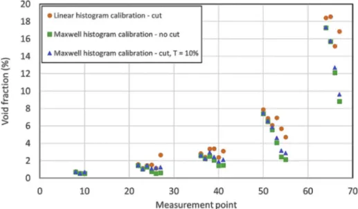
All measurement points were tested with threshold values ranging from 10% to 50% with increments of 5%. Increasing the threshold will result in having less bubble connected values and thus fewer subtracted negative values from the initial detected negative matrix. Eventually, if the threshold is too high the filter would start to remove negative points on bubble edges. Thus, the estimation of the threshold value was done empirically using the appearance of negative cross-sectional averaged void fractions according to eq. (8). The best results were obtained having threshold values starting from 10% to 30%. For further calculation and comparison, we will use 10% as a threshold. This value removes 99% of all negative values from the frame averaged void fractions, without ignoring too many smaller bubbles. Therefore, we will use this value as a compromise and call this method the Maxwell histogram calibration – conditional cut 10%.
The results obtained with different methods of calculating the mean void fractions are visualized in Fig. 9. Each of the five clusters corre-sponds to a constant superficial gas velocity and, when going from left to right, represents the measurement points in order of increasing super-ficial liquid velocity, i. e. horizontal transitions from plug to bubbly region in Fig. 3. As the calibration file method can lead to inaccurate results, all mean void fractions were calculated on the basis of histogram calibration using the corresponding raw data from the measurement file. The differences in void fraction between all three methods is almost negligible for the left points in each cluster, i. e. for the points being most likely associated with plug flow scenarios. Most noticeable differences
can be seen for the right points in each cluster, which correspond to bubbly flows, as well as transitional ones. As in agreement with Prasser’s experiment [15], the linear–cut method has higher void fraction compared to the other two, due to overestimation of bubble sizes. The difference between both Maxwell methods depends on the threshold. Maxwell’s method without excluding any negative value is producing a certain number of frames with negative values of cross-sectionally averaged void fraction. Negative void fractions across an entire frame represent physically inacceptable results and can thus not be used. Therefore, we use the newly introduced method with conditional cut featuring a threshold of 10% for all further analyses.
4.2. Analysis of gas core behavior
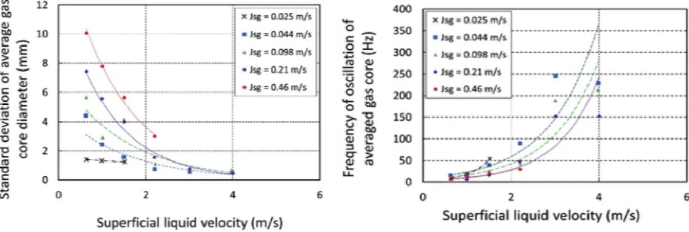
Fig. 10 shows the average diameter of the gas core for variation of superficial liquid and gas velocities. Expectedly, the average core diameter generally increases with rising superficial gas velocity, or more precisely higher gas flow rate. However, the behavior with respect to the superficial liquid velocity is not uniform. While lower gas flow rates show increasing core diameters with increasing liquid flow rates, the opposite trend is obtained for the highest superficial gas velocity of Jsg ¼ 0.46 m/s. Additionally, the core diameter obviously tends to get almost independent of the gas flow rate at higher superficial liquid velocities. In
Fig. 9. Mean void fraction obtained by different methods. Measurement points taken from Fig. 3. “T” is the threshold number.
Fig. 10. Average gas core diameter in dependence of superficial velocities of
order to interpret these results, two aspects need to be considered. Firstly, the influence of the upstream flow morphology must be taken into account. All of the investigated operation points are located in the plug region or in the transition region between plug and bubbly flow (Fig. 3). Here, an increasing liquid flow rate leads to rising shear stresses resulting in breakage of larger gas plugs. This is associated with the occurrence of more frequent and smaller voids, i. e. a higher level of gas dispersion, as confirmed by Fig. 11 showing at the standard deviation and frequency of void fraction fluctuations.
As the standard deviation of void fraction fluctuation at low super-ficial gas velocities does not change significantly with supersuper-ficial liquid velocity and shows comparable values to those of the bubbly regime at maximum liquid flow rates, an overall more bubbly than intermittent character can generally be assumed for these small gas flow rates. In contrast, the regime transition from plug to bubbly flow is more relevant in case of higher superficial gas velocities. Regarding the frequency of void passage, the generally expected behavior is observed in Fig. 11, but no clear differences can be detected with respect to the investigated gas velocities.
The corresponding downstream behavior after passage of the swirl element is depicted in Fig. 12 and shows comparable results. For all investigated superficial gas velocities, decreasing amplitudes and increasing frequencies of the core diameter fluctuations are observed with increasing liquid velocity. Both result from the more dispersed gas phase and thus the more homogeneous phase distribution at the stage of entering the core, which leads to less intense disturbances of the swirling flow structure. Note that the standard deviation of core fluctuations in Fig. 12 reaches values of less than 1 mm in the bubbly regime. For practical application the necessity of applying dynamic control to the separation process is thus of greater importance for predominantly
intermittent flow patterns, i. e. at lower superficial liquid velocities and/ or higher superficial gas velocities.
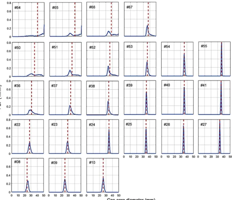
With that in mind, it seems not sufficient to focus on temporal av-erages only in order to explain the inverse trends of the average core diameter in dependence of the gas flow rate in Fig. 10. Therefore, Fig. 13 depicts the probability density functions (PDFs) of the time series of the calculated core diameters for all experimental points.
Whereas most of the PDFs are characterized by a single distinct peak being associated with a stable core, points 50 to 52 and 64 to 67 show significantly broader and largely also flatter distributions of gas core diameters. Here, an increasing probability of the occurrence of large core diameters is observed with increasing intermittent character of the upstream flow pattern, i. e. at lower superficial liquid velocities and/or higher superficial gas velocities cf. fig. 10. Moreover, the core even reaches the inner pipe diameter for points 64 to 66 indicating in-terruptions of the liquid film.
Besides the influence of the upstream flow pattern, a stabilization of the gas core is generally observed with increasing superficial liquid velocity. The change in pressure difference within each fluid in radial direction downstream is much smaller than the actual difference be-tween the two fluids according to Slot [16]. The highest pressure is measured close to the swirl element near the wall, while the lowest pressure is close to the swirl in the center. Due to much higher difference in pressure between the fluids, the increase in gas flow will not allow the gas core to expand further even if the initial void fraction of the up-coming flow is higher. Moving further downstream this effect of pres-sure difference and losing momentum will be less due to friction. The two separated fluids would eventually merge downstream, thus the reason for mounting the camera near the swirl element. However, the gas core diameter also expands having lower superficial gas velocity
Fig. 11. Standard deviation (left) and frequency (right) of upstream void fraction fluctuations in dependence of superficial velocities of liquid and gas.
while gradually increasing superficial liquid velocity.
According to the findings of Slot [16] the pressure inside the core is larger at lower superficial liquid velocity than at higher for single phase flow. The only difference between single- and two-phase flow in pres-sure magnitude is the less steep increase in magnitude in radial direction from the center for two phase flow. Wall pressure and thus the pressure difference between separated fluids downstream increases in magnitude while having higher liquid flow. These conditions are enabling the gas core to expand by having constant lower gas flow and continues increase in liquid flow. This behavior also reaches saturation in gas core expan-sion as the type of incoming flow becomes bubbly.
In summary, two main aspects were identified to have impact on the behavior of the gas core: (1) The upstream flow pattern strongly in-fluences the stability of the core. Large fluctuations of the diameter are observed in case of intermittent flows whereas bubbly flows generally produce more stable cores. (2) An increasing liquid flow rate leads to decreasing influence of the gas flow, since the swirling flow pattern is liquid dominated. At high superficial liquid velocity, the core diameter gets almost independent of the gas flow in the observed region.
4.3. Upstream-downstream correlation
Despite the overall stable behavior of gas cores in case of bubbly flow in the upstream section, a varying average diameter is observed with respect to changing operating conditions, cf. figure 10. Since the devi-ation around the arithmetic mean is rather small in these cases, as shown in Fig. 12, we propose correlating the average core diameter with up-stream data from the wire-mesh sensor in order to provide an empirical basis for controlling the separation efficiency in this flow regime. This has been done on both plug and bubbly flow. The experimental data showed a relation of the average core diameter and the mean upstream void fraction. Functions that gave best qualitative agreement and were used for empirically fitting are
dBUBBLY¼1:76 lnðεÞ þ 33:953; R2¼ 0:7477 (21)
dPLUG¼4:48 lnðεÞ þ27:306; R2¼ 0:9282 (22) where d is the averaged core diameter calculated from processed camera recordings, ε the void fraction obtained from the wire-mesh sensor and
Fig. 13. Probability density function (solid line) and arithmetic means (dashed line) of core diameter fluctuations (arrangement according to operation points
R2 the coefficient of determination showing similarities between data sets. The results are depicted in Fig. 14 where certain points were grouped into bubbly and plug flow. The selection for grouping was based on the position of the measurement points on the flow map in Fig. 3 and the recorded cross-sectional depiction of the flow using the wire-mesh sensor.
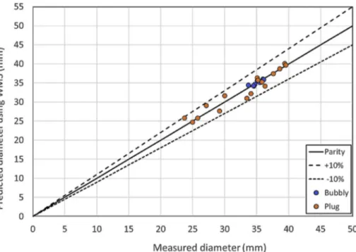
In order to evaluate the quality of the proposed empirical correla-tion, the gas core diameters were recalculated based on the logarithmic function and measured void fractions. They are plotted against the experimental core diameters from high-speed camera measurement in Fig. 14. The predictions agree well within a relative error of � 10% for both types of flow as shown in Fig. 15. The empirical correlation can thus be used in control systems when bubbly flow patterns are present in the upstream section. However, systems that are more sophisticated are still required in order to enable highly dynamic control in case of strong
variations with intermittent upstream patterns. This will be objective of future studies.
5. Conclusion
This work was focused on finding the behavior of upstream and downstream conditions in an inline-fluid separator. More precisely, the behavior of downstream vortex shaped gas core in dependence of up-stream multiphase flow of air and water under different flow rates.
Maxwell model was used to increase the accuracy of local instanta-neous void fraction calculation. Detection and removal of negative void fractions in the bulk region using an empirically calculated threshold of 10% has shown the most accurate physical representation of the gas hold in a cross section. Therefore, the Maxwell histogram calibration – conditional cut with a threshold level of 10% is the method with highest
Fig. 14. Relationship between upstream void fraction and downstream core diameter.
possibility of estimating the gas hold up in our inline fluid separation process.
After observations and calculations, we have concluded that super-ficial gas and liquid velocities, void fraction and the type of incoming multiphase flow are the main parameters to estimate gas core properties such as average diameter over time and stability. Variables created as an output from processed camera images gave information about the pro-duced vortex shaped gas core downstream. The decreased standard deviation and frequency of fluctuation is a good indication for stability of the gas core.
Calculated correlation from upstream and downstream measure-ments proved that the wire-mesh sensor has a high potential for esti-mating the average gas-core diameter downstream. More investigations have to be done for different flow conditions, which will allow us to establish an empirical relation for the WMS leading to improvement in estimation for the gas core shape and behavior. One of the upcoming tasks will be to calculate the split efficiency of the system by measuring the gas carry over and water carry under. These results will in the future help to develop a control system for increasing the separation efficiency of an inline fluid separator.
Acknowledgement
This project has received funding from the European Union’s Hori-zon 2020 Research and Innovation Program under the Marie Sklodowska-Curie grant agreement No. 764902.
References
[1] H. Veldman, G. Lagers, 50 Years Offshore (Handbook), Foundation of Offshore Studies, Delft, 1997.
[2] H. Devold, Oil and Gas Production (Handbook), ABB Oil and Gas, Oslo, 2013. [3] J. Veil, J. Quinn, Water Issue Associated with Heavy Oil Production, Argone - U. S.
Department of Energy, Chicago, 2008.
[4] J. Yin, J. Li, Y. Ma, H. Li, W. Liu, D. Wang, Study on the air core formation of a gas–liquid separator, J. Fluid Eng. 137 (2015).
[5] L. Van Campen, Bulk Dynamics of Droplets in Liquid-Liquid Axial Cyclones (Ph.D. dissertation), TU Delft, Delft, 2014.
[6] S.M. Huang, C.G. Xie, R. Thorn, D. Snowden, M.S. Beck, Design of sensor electronics for electrical capacitance tomography, IEEE Proc.-g 139 (1) (February 1992).
[7] M. Da Silva, E. Schleicher, U. Hampel, Capacitance wire-mesh sensor for fast measurement of phase fraction distributions, Meas. Sci. Technol. 18 (2007) 7. [8] P. Wiedemann, A. D€oß, E. Schleicher, U. Hampel, Fuzzy flow pattern identification
in horizontal air-water two-phase flow based on wire-mesh sensor data, Int. J. Multiphas. Flow 117 (2019) 153–162.
[9] J.M. Mandhane, G.A. Gregory, K. Aziz, A flow pattern map for gas/liquid flow in horizontal pipes, Int. J. Multiphas. Flow 1 (1974) 537–553.
[10] N. Otsu, A threshold selection method from gray-level histograms, IEEE Trans. Syst. Man Cyber. 9 (1979) 62–66.
[11] Matlab, Image Processing Toolbox R2018a, Mathworks, Natick, 2018. [12] H.-M. Prasser, A. B€ottger, J. Zschau, A new electrode-mesh tomograph for gas/
liquid flows, Flow Meas. Instrum. 9 (1998) 111–119.
[13] H.-M. Prasser, A. B€ottger, J. Zschau, A New wire-mesh tomograph for gas liquid flows, in: F.-P. Weiß, U. Rindelhardt (Eds.), Annual Report 1996, Institute for Safety Research, FZR-190, 1997, pp. 34–37.
[14] M. Beyer, L. Szalinski, E. Schleicher, C. Schunk, WMS-software User Manual v1.3, Helmholtz-Zentrum Dresden-Rossendorf, Dresden, 2012.
[15] H.-M. Prasser, Signal response of wire-mesh sensor to an idealized bubbly flow, Nucl. Eng. Des. 336 (2018) 3–14.
[16] J. Slot, Development of a Centrifugal Inline Separator for Oil-Water Flows, University of Twente, Enschede, 2013 (Ph.D. dissertation).