Évolution des principes de la conception des réseaux de neurones artificiels

THÈSE

En vue de l’obtention du

DOCTORAT DE L’UNIVERSITÉ DE TOULOUSE

Délivré par l'Université Toulouse 3 - Paul Sabatier

Présentée et soutenue par

Dennis WILSON

Le 4 mars 2019

Évolution des principes de la conception des réseaux de neurones

artificiels

Ecole doctorale : EDMITT - Ecole Doctorale Mathématiques, Informatique et

Télécommunications de Toulouse

Spécialité : Informatique et Télécommunications Unité de recherche :

IRIT : Institut de Recherche en Informatique de Toulouse

Thèse dirigée par

Hervé LUGA et Sylvain CUSSAT-BLANC

Jury

M. Marc Schoenauer, Rapporteur M. Keith Downing, Rapporteur Mme Una-May O'Reilly, Examinatrice

Mme Sophie Pautot, Examinatrice Mme Anna Esparcia-Alcázar, Examinatrice

Mme Emma Hart, Examinatrice M. Hervé LUGA, Directeur de thèse M. Sylvain Cussat-Blanc, Co-directeur de thèse

Dennis G. Wilson

February 28, 2019

The biological brain is an ensemble of individual components which have evolved over millions of years. Neurons and other cells interact in a complex network from which intelligence emerges. Many of the neural designs found in the biological brain have been used in computational models to power artificial intelligence, with modern deep neural networks spurring a revolution in computer vision, machine translation, natural language processing, and many more domains.

However, artificial neural networks are based on only a small subset of biological functionality of the brain, and often focus on global, homogeneous changes to a system that is complex and locally heterogeneous. In this work, we examine the biological brain, from single neurons to networks capable of learning. We examine individually the neural cell, the formation of connections between cells, and how a network learns over time. For each component, we use artificial evolution to find the principles of neural design that are optimized for artificial neural networks. We then propose a functional model of the brain which can be used to further study select components of the brain, with all functions designed for automatic optimization such as evolution.

Our goal, ultimately, is to improve the performance of artificial neural networks through inspiration from modern neuroscience. However, through evaluating the bio-logical brain in the context of an artificial agent, we hope to also provide models of the brain which can serve biologists.

Le cerveau biologique est composé d’un ensemble d’éléments qui évoluent depuis des mil-lions d’années. Les neurones et autres cellules forment un réseau complexe d’interactions duquel émerge l’intelligence. Bon nombre de concepts neuronaux provenant de létude du cerveau biologique ont été utilisés dans des modèles informatiques pour développer les algorithmes dintelligence artificielle. C’est particulièrement le cas des réseaux neuronaux profonds modernes qui révolutionnent actuellement de nombreux domaines de recherche en informatique tel que la vision par ordinateur, la traduction automatique, le traitement du langage naturel et bien d’autres.

Cependant, les réseaux de neurones artificiels ne sont basés que sur un petit sous-ensemble de fonctionnalités biologiques du cerveau. Ils se concentrent souvent sur les fonctions globales, homogènes et à un système complexe et localement hétérogène. Dans cette thèse, nous avons d’examiner le cerveau biologique, des neurones simples aux réseaux capables d’apprendre. Nous avons examiné individuellement la cellule neuronale, la for-mation des connexions entre les cellules et comment un réseau apprend au fil du temps. Pour chaque composant, nous avons utilisé l’évolution artificielle pour trouver les principes de conception neuronale qui nous avons optimisés pour les réseaux neuronaux artificiels. Nous proposons aussi un modèle fonctionnel du cerveau qui peut être utilisé pour étudier plus en profondeur certains composants du cerveau, incluant toutes les fonctions conçues pour l’optimisation automatique telles que l’évolution.

Notre objectif est d’améliorer la performance des réseaux de neurones artificiels par les moyens inspirés des neurosciences modernes. Cependant, en évaluant les effets biologiques dans le contexte d’un agent virtuel, nous espérons également fournir des modèles de cerveau utiles aux biologistes.

A thesis can sometimes appear a solitary endeavor and is certainly a reflection of the au-thor’s interests, methods, and understandings. In truth, this thesis has been anything but solitary, with numerous actors influencing not only the work presented in this thesis, but also myself, and my own interests, methods, and understandings. I want to acknowledge a select few, although many others remain unacknowledged but greatly appreciated.

My advisors, Sylvain Cussat-Blanc and Hervé Luga, have shaped, supported, and challenged every idea in this document, working with me tirelessly to guide my sometimes circuitous exploration of interests. They have also supported and challenged me as a person, guiding my growth and change these past three years. It isn’t simple moving to a new continent and adapting to a new university, culture, and bureaucracy, and I’ve only made it to this final stage of my thesis thanks to their extensive and comprehensive support.

Along the way, I was fortunate to gain another advisor in all but name, Julian Miller. He has been a source of insight in our collaborations, and his passion for researching interesting topics, irrespective of their current difficulty or popularity, has inspired me and encouraged my own research directions.

The jury of this thesis have all also influenced it and me in various ways. Keith Downing’s book, Intelligence Emerging, set the direction for much of this thesis and encouraged my interest in artificial life. My first experience with live neurons was in Sophie Pautot’s lab, where I learned how much of a mystery neurons still are. The works of Marc Schoenauer, Emma Hart, and Anna Esparcia have all inspired and informed me, and a motivation to see and maybe impress them has pushed a number of the GECCO articles in this thesis through to completion. Finally, none of this would have happened without Una-May O’Reilly, who took in a somewhat lost sophomore, showed me the marvels of bio-inspired computing, and encouraged me to pursue a PhD in this field.

To all of the above, I express my deep gratitude for their impact on this thesis, whether direct or indirect, and on me. I can only hope to someday impact the research and life of another as they have mine.

1 Introduction 11

1.1 The brain as a model . . . 14

1.2 Evolving emergent intelligence . . . 15

1.3 Organization of the thesis . . . 17

2 Background 19 2.1 Neural cell function . . . 21

2.1.1 Biological neural models . . . 22

2.1.2 Activation functions . . . 24

2.1.3 Other cell behavior in the brain . . . 26

2.2 Neural connectivity . . . 26

2.3 Learning in neural networks . . . 29

2.3.1 Spike Timing Dependent Plasticity . . . 30

2.3.2 Gradient Descent and Backpropagation . . . 32

2.4 Evolutionary computation . . . 33

2.4.1 Evolutionary strategies . . . 34

2.4.2 Genetic Algorithms . . . 34

2.4.3 Genetic Programming . . . 36

2.5 Evolving artificial neural networks . . . 36

2.6 Objectives of the thesis . . . 38

3 Evolving controllers 41 3.1 Artificial Gene Regulatory Networks . . . 42

3.1.1 AGRN applications . . . 43

3.1.2 AGRN overview . . . 45

3.1.3 AGRN dynamics . . . 47

3.1.4 AGRN experiments . . . 50

3.1.5 AGRN results . . . 52

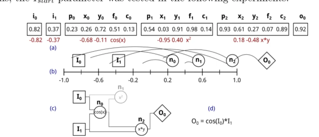
3.2.1 CGP representation. . . 59

3.2.2 Playing games with CGP. . . 60

3.2.3 Positional Cartesian Genetic Programming . . . 65

3.2.4 Genetic operators for CGP . . . 66

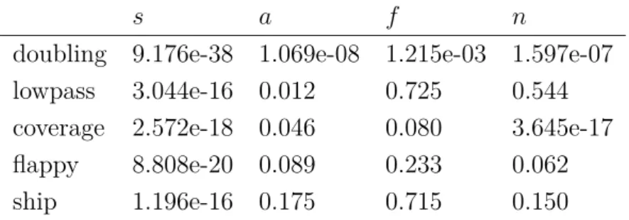
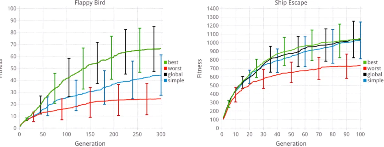
3.2.5 CGP experiments . . . 68

3.2.6 CGP method comparison. . . 69

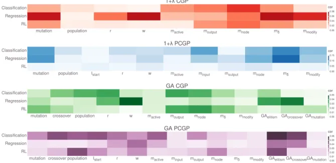
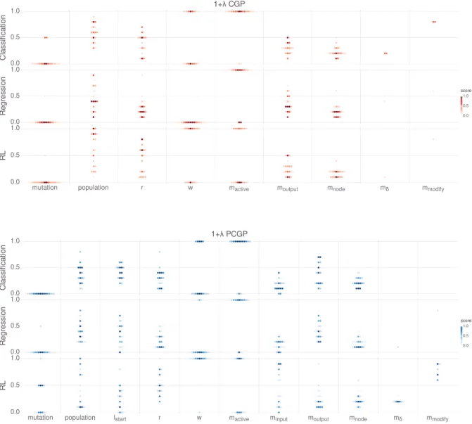
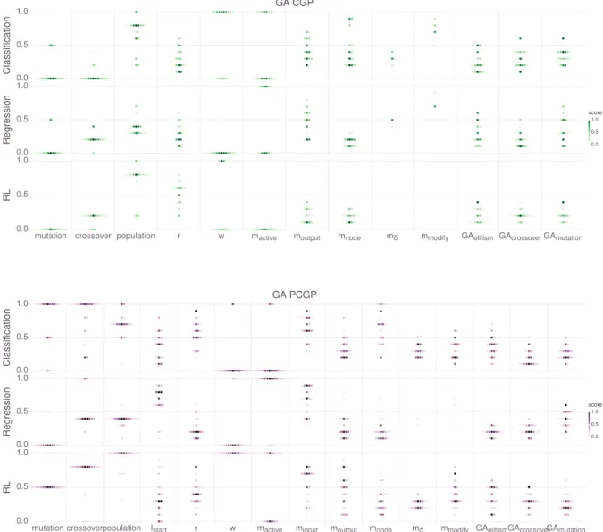
3.2.7 CGP parameter study . . . 71

3.3 Conclusion . . . 74

4 Evolving neural cell function 77 4.1 Spiking neural activation functions . . . 78

4.2 Neural network model . . . 81

4.3 Experiment . . . 83 4.3.1 Clustering tasks . . . 83 4.3.2 Network . . . 84 4.3.3 Training . . . 84 4.3.4 Evolution . . . 85 4.4 Results . . . 86 4.5 Conclusion . . . 87

5 Evolving developmental neural connectivity 91 5.1 Biological axon development . . . 93

5.2 Axon guidance model . . . 97

5.2.1 Cellular models . . . 97

5.2.2 Environment initialization . . . 99

5.2.3 Environment update . . . 99

5.2.4 Model configuration and evolution. . . 101

5.3 Eye-specific patterning . . . 102

5.3.1 Visual system environment . . . 102

5.3.2 Evolutionary results . . . 104

5.4 Robot coverage . . . 108

5.5 Conclusion . . . 111

6 Evolving learning methods 113 6.1 Reward-Modulated Spike-Timing Dependent Plasticity . . . 117

6.1.1 Neuron and learning models . . . 118

6.1.2 Neuromodulation reward model . . . 119

6.1.3 Instrumental conditioning . . . 121

6.1.5 Evolution of neuromodulation method . . . 125

6.1.6 Evolution results . . . 126

6.1.7 Summary of Reward-Modulated STDP . . . 128

6.2 Neuromodulation of learning parameters in deep neural networks. . . 128

6.2.1 AGRN neuromodulation model . . . 130

6.2.2 Evolution of the neuromodulatory agent . . . 132

6.2.3 Comparison of neuromodulation to standard optimization . . . 135

6.2.4 Generalization of the neuromodulatory agent . . . 136

6.2.5 Neuromodulation behavior . . . 138

6.2.6 Summary of neuromodulation of learning parameters in deep ANNs 139 6.3 Conclusion . . . 141

7 Discussion and conclusion 143 7.1 A framework for developmental neuroevolution . . . 146

7.2 Evolving to learn for data classification . . . 149

7.3 The evolution of learning . . . 150

Introduction

Chlamydomonas reinhardtii is a type of single-celled freshwater green alga. This

sim-ple organism uses two flagella to propel itself through water, guided by photosensory, mechanosensory, and chemosensory cues. Membrane receptors located in the cell body detect sensory input, which leads to membrane depolarization and moves the cilia located on the cell body. This sensor-actuator system allows C. reinhardtii to navigate through ever-changing environments. The mechanism responsible for sensing the environment and sending information to other processes in the cell is the transient receptor potential (TRP) channel. These ion channels in C. reinhardtii share features with the TRP channels used

by mammals in the sensory system [Ari+15]. This suggests that the TRP channel gating

characteristics, used in the human brain, evolved early in the history of eukaryotes. Single-celled organisms have also been shown to be capable of learning and having memory. This has mostly been demonstrated in ciliates, organisms which move using

small hair-like cilia on the outside of the cell. In [Woo88], Wood showed that repetitive

mechanical stimulation of Stentor leads to contraction becoming more and more common in the cell. The contraction response following the first input of mechanism stimulation disappeared after this input was gone, but the memory of the event was intact. When inputs of the same type were given, the contraction response was facilitated. Paramecium, a well-known freshwater ciliate, has been shown to be capable of learning to associate

between light and electrical stimulations [AMJ06].

In unicellular organisms, sensors and actuators are part of the same cell, while in multicellular neuronal organisms the two components reside in different, sometimes very distant, cells. Nevertheless, in both cases the molecular machinery underlying the

learn-ing phenomena are basically the same [GJ09]. The cellular mechanisms that serve as

building blocks of the brain were created by evolution long before the first organism with a brain, even before the first mammals. The cells of the brain, neurons, oligodendrocytes, astrocytes, and others, have evolutionary precursors and use mechanisms shared by other

Figure 1.1: Scanning electron microscope image of Chlamydomonas reinhardtii, a unicellular flagellate used as a model system in molecular genetics work and flagellar motility studies.

cells and other organisms. Their form in the mammal and human brain is the result of a long evolutionary process of refinement, even before they were composed into nervous systems.

In neural organisms, those with a nervous system, neurons act as the medium of in-formation transportation from sensors to actuators, as well as the regulators of biological processes. In C. elegans, a microscopic worm, the nervous system is used to control the movement of the worm and for triggering digestive processes, and uses information from the digestive system to influence the worm’s movement, deciding whether it is roaming to find new food or grazing in a specific spot. The C. elegans nervous system is shown

inFigure 1.2. While the acts of this nervous system are far from meeting modern

defini-tions of intelligence, the brain of the C. elegans resembles our own in many ways [IB18].

Evolution has selected neural designs for the worm suited for its needs and environment by shaping the worm’s genes, which in turn decide how the worm’s neurons develop, act, connect, and learn.

The neural designs created by evolution are as remarkable as they are a mystery. A

bee with only 106 neurons can learn to break camouflage, navigate a maze via symbolic

cues, and perform cognitive tests that were thought, until recently, impossible except

for in monkeys, humans, dolphins, and pigeons [SL15]. To do this, the relatively small

number of cells must be used efficiently, and the neural designs found in biology use a variety of information passing mechanisms to ensure the best use of these cells.

Neurons primarily communicate with electrical signals, by sending electrical spikes down long, branching axons similar to insulated wires. This rapid information transfer

allows for information to travel through the brain at 1 mm per ms [SL15]. Chemical

ganglia, including the retrovesicular ganglion (RVG) and ventral ganglion (VG). Full image and more information on C. elegans are available at www.wormatlas.org

passed locally or slowly, at around 1µm per ms. However, chemical signaling is much less expensive in terms of energy and requires less organization; multiple cells can be reached at the same time by using a diffusive signal. The design of using chemical signaling for some communication and wired signaling for other is one which has been optimized over the course of evolution. In C. elegans, chemical signals are the primary form of communication, while in humans, myelinated (insulated) wires traverse the nervous sys-tem and throughout the brain, with chemical signals distributing reward information and activating motor responses.

Evolution has found these designs through millions of years of trial and error. From mechanisms that allowed C. reinhardtii to sense the direction of light and C. elegans to search for food, complex brains have arisen. Some of these elements have persisted from the simplest organisms throughout all intelligent ones, such as the ion channels employed by the C. reinhardtii. Light-sensing cells in the eye, on the other hand, were found by evolution multiple times in distinct cases. The octopus and the mammal diverged 500 million years ago in evolution, and the octopus brain is very different from the mammal brain, with a processing center in each arm as opposed to one central brain. However,

the two organisms respond to seratonin, a neurotrasmitter, in similar ways [ED18]. Some

principles of neural design are seemingly inherent; they are concepts that are so beneficial that they are found multiple times by evolution.

In this work, we aim to understand these aspects of neural design as they apply to Artificial Neural Networks (ANNs). Just as these designs were found by evolution, we use artificial evolution to discover neural designs fit for computational tasks. In simulation, many of the physical principles encountered by biological evolution aren’t present. Dif-fusive communication, done with a chemical in biology, is more expensive in simulation than wired communication, not less. Information can be passed between artificial neurons instantaneously, so the speed of information travel is not a consideration. The evolution of neural design for artificial neurons must therefore follow different principles than that of

biological evolution. However, we use biological neurons, from the simple networks found in C. elegans to the complex ones in the human brain, as inspiration for our artificial models. In the next section, we will briefly describe the history of ANNs inspired by the biological brain.

1.1

The brain as a model

The earliest model of the brain comes from the McCulloch-Pitts neuron model, devel-oped in 1943 [mcculloch_logical_1943-1]. The motivation for the development of this model was in understanding the biological brain. Recent biological experiments had allowed for the collection of neural activity data, which was then used to create the mathematical model in a foundational moment for the field now known as computational neuroscience. However, the idea of simulating the biological brain soon caught the interest of those in the nascent field of computation. In 1954, an ANN capable of learning was simulated. This network used Hebbian learning, where correlated activity between any

two neurons in a network reinforced the connection between them [FC54]; this concept

had only recently been discovered in biology. Soon after, the perceptron model was

cre-ated [Ros58], an abstract model of the neuron based on average spiking activity. This

model was very popular in the new field of artificial intelligence for almost a decade, until various shortcomings led researchers to other models. The most well-known of these is the inability of the perceptron to calculate the exclusive-or function, described by Minsky

in 1969 [MP69].

Almost a decade later, artificial intelligence research once again focused on ANNs.

The backpropagation algorithm, from [Wer74], allowed for layers of perceptrons to be

trained, fixing some of the earlier problems with the model. Schmidhuber showed that the same Hebbian learning principles used 40 years earlier could improve ANN learning

by pre-training individual layers before using backpropagation [Sch92]. However, the

prohibitive costs of training these multi-layer perceptrons discouraged their use. Other methods dominated the field of artificial intelligence, such as expert systems of conditional statements, based on the mathematics branch of logic.

After another two decades, ANNs were shown to solve problems in image recognition,

greatly outperforming other methods of the time [Kri+12]. These deep neural networks

somewhat resembled the perceptron models of the past, in that individual neurons sim-ulated average activation and used a single synaptic connection to express the average connection with another neuron. However, their organization in layers gave them a con-siderable advantage over previous models. Some layers fixed weights in kernels, creating a convolutional function that added shift invariance during training, an idea inspired by image processing algorithms. Other layers condensed information by taking the

maxi-mum of different neural activations, or the average. This was an early work in the now

ubiquitous field of deep learning [LBH15].

Meanwhile, the field of neuroscience has made enormous progress in understanding the brain. The Hebbian learning process was defined more specifically, and the Hebbian process of synaptic efficacy change, Spike-Timing Dependent Plasticity, was discovered

[CD08a]. Other cells besides neurons were shown to play important roles in the brain;

astrocytes, a type of glial cell, were shown to induce neurogenesis, the creation of new

neurons [SSG02]. Developmental processes such as axon guidance were traced from the

molecular level to the cellular to understand their underlying mechanisms [Chi06]. Other

computational neural models were created such as the Hodgkin-Huxley model, developed

in 1952 [HH52], and the Hindmarsh-Rose model in 1984 [HR84].

Some of these ideas have been integrated into modern artificial neural networks. The neurons in most deep neural networks employ a rectified linear unit function, which has

a basis in biology [Hah+00]. One of the inspirations for organizing neurons into layers

came from the organization of neurons in cortical columns in the visual system of the brain

[LBH15]. However, other ideas from modern neuroscience have yet to be explored. Almost

all ANNs use exclusively neural cells, where other types of cells have been shown to play

an important role in neural function [Por+11]. ANNs generally use a fixed architecture,

where connections between neurons are defined at initialization and don’t change, but

topological changes have been shown to play an important role in learning [MW17].

The biological brain and the nervous system can inform many of the choices made in artificial neural design. The mechanisms which make biological brains incredibly complex are the same mechanisms responsible for making them efficient computing machines. The biological brain uses 100,000 times less space and energy than a computer, and can perform

feats not yet possible with artificial intelligence [SL15]. Bees can learn to do tasks only

recently accomplished by deep reinforcement learning, and artificial cognition remains a distant goal. To improve ANNs, and to gain a better understanding of the biological brain, it is worth exploring the details of biological neural design.

In this work, we focus on the integration of recent neuroscience into artificial models. We explore axon guidance, glial cell function, and dopamine signaling in the context of ANNs. Some of these components, i.e. axon guidance, are not yet fully understood in biology. This work can therefore serve both purposes, to increase biological understanding and to improve ANNs, although our focus is on using ANNs for computational tasks.

1.2

Evolving emergent intelligence

In choosing the focus of study and the design of models in this work, certain guiding principles were followed. The use of modern neuroscience is one such principle. The

other main principle is a focus on emergence, the formation of global patterns from solely local interactions. In the brain, no single neuron is responsible for intelligence, nor does individual synaptic behavior represent an idea or thought. Instead, the intelligence of the brain is the result of the interaction between neurons; it emerges from the complex web of neural and synaptic interaction.

Emergent behavior has many examples in biology besides the brain. Ants collectively find optimal paths between their colony and a food source by communicating via chemical traces on the ground. Termites construct nests with specialized structures and intricate

tunnels by collectively following the same set of simple rules [Bon+99]. These

organ-isms have served as inspiration for artificial intelligence, notably in the field of swarm intelligence. In this work, we focus on the emergent behavior of neural systems.

In [Dow15], Downing provides a common framework for emergent artificial intelligence:

• Individual solutions to a problem (building an intelligent system) are represented

in full. Each solution is an agent.

• Each agent has a genotype and a phenotype

• Each agent is exposed to an environment, and their performance within it is assessed. • Phenotypes have adaptive abilities that come into play during their lifetime within

the environment. This may improve their evaluation, particularly in environments that change frequently, throwing many surprises at the phenotypes.

• Phenotypic evaluations affect the probabilities that their agents become focal points

(or forgotten designs) of the overall search process

• New agents are created by combining and modifying the genotypes of existing

agents, then producing phenotypes from the new genotypes.

This framework can be seen as a guide to process used in the following chapters. Agents are evolved, and specific attention is given to the genotype representations to improve evolution. These agents act in environments to control the behavior or interactions of neurons, and the performance of the agents influences their evolutionary success.

To focus on emergence, we design agents for local interaction. These individuals

inform the rules of local interactions in a neural network. The neural network is then evaluated for its capacity to learn, which is the evolutionary fitness then assigned back to the individual agent. The genotype of the agents can be seen as a part of the genome of neural design, deciding how a specific mechanism of the neural network functions.

1.3

Organization of the thesis

In this work, we use evolution to apply biologically inspired concepts to artificial neu-ral design. To study the entire design of the neuneu-ral network, we consider the different mechanisms of neural network functions in three separate components:

• cell function, how individual neurons behave • neural connectivity, how neurons form connections • learning, how neurons and connections change over time

We focus on the evolution of each of these components individually, and then consider them all together in a final model. This allows us to understand the importance of each part of a neural network and the challenges presented by the design of each component.

In the next chapter, we present an overview of each neural component, starting from their biological basis and exploring existing work to model them. We consider the full range of abstraction, from biological models that attempt to simulate reality to artificial models only vaguely inspired by these components. Each neural component is presented separately, so some models, such as deep learning, are presented in different contexts for the different components.

We conclude chapter 2 with an overview of artificial evolution. Following Downing’s

framework, the individuals in our evolutionary algorithms are agents. Unlike the evolu-tion of a direct soluevolu-tion to a problem, the evoluevolu-tion of agents or their controllers involves

specific techniques and challenges. We explore the evolution of agent controllers in

chap-ter 3. Specifically, in this work we use two mediums for agent evolution, Artificial Gene

Regulatory Networks (AGRN) and Cartesian Genetic Programming (CGP), which are

presented in detail inchapter 3.

The behavior of individual neurons is examined in chapter 4. We explore existing

models of spiking neurons and propose a new design goal for these models: increased fitness during learning. We evolve new spiking neural functions for this goal on a data clustering task. The learning method and neural architecture are fixed to understand how the neural behavior alone impacts learning.

Next, a study in neural connectivity is presented in chapter 5. We construct a model

of axon guidance with evolved agents controlling axon behavior and the diffusion of chem-ical guidance cues throughout the environment. The agents are evolved to create topol-ogy with specific traits, such as high symmetry, and to perform in artificial tasks. We demonstrate that the axons rely on neural activity for guidance, a principle only recently discovered in biology.

The final component, learning, is covered inchapter 6. We focus on neuromodulation,

behavior. To cover this vast topic, we present two separate studies. In the first, a dopamine signal is modeled to impact the Hebbian change in the neural networks of virtual creatures learning to swim. In the second, learning in deep neural networks is augmented by local changes to learning rate and synaptic weight update made by neuromodulatory agents placed throughout the network.

In chapter 7, these three neural components are brought together. A complete model

of a neural network is presented, where each part of the network is controlled by evolved agents. Each agent is responsible for a function of the network, like the individual compo-nents presented here. The genes of these agents are represented as separate chromosomes of the evolved agent, allowing for specific study of certain functions or evolution of the entire agent.

The objective of this work is to discover, through evolution, the important principles of artificial neural design. In the biological brain, the same design principles are used across different components. For example, redundancy of information is used to combat the noise of stochastic biological processes at the level of individual synapses but also at the level of brain organization. By studying artificial neural design in different neural components, we can gain insight into the design principles that are general across all parts of an ANN, as well as those which are important for each component individually.

Background

The brain has long been a source of inspiration for computational intelligence. In 1948,

Turing developed B-type machines based on neurons [Tur09], and in 1954, Farley and

Clark simulated a network based on the recently founded Hebbian theory [Heb+49],

[FC54]. Perceptrons popularized the use of artificial neural networks for computational

tasks as early as 1958 [Ros58].

Since then ANNs have risen and fallen in use as artificial controllers. Modern ANNs have recently demonstrated human-level ability, and in some cases, super-human ability,

in image recognition [Kri+12], game playing [Mni+15], text translation, [Fir+17], speech

recognition [Dah+12], and more [DY+14]. This is largely due to the advent of deep

learning, a machine learning field which optimizes deep neural networks for specific tasks

[LBH15]. Deep learning is the state of the art for a large amount of research using

artificial neural networks, and in this thesis we use deep learning to study neuromodulation (section 6.2).

However, for the most part, the models in this work are based on spiking neural

net-works, which have only recently been used in ways that resemble deep learning [Khe+16],

but which have also demonstrated impressive ability for application [Moz+18a], [LDP16].

The presentation of deep learning concepts in this chapter is therefore minimal; we in-stead focus on how biological neurons have influenced a variety of artificial neural network models, including but not limited to deep learning.

The neuron is the base unit of computation in the biological brain. A schematic of

the neuron is shown in Figure 2.1, displaying the different components of the neuron.

The cell body of the neuron, the soma, extends multiple projections, the morphology of which depends on the specific neuron type. In the development of the neuron, one of these projections becomes an axon, which serves as output for the neuron. All other projections become dendrites, which provide input to the neurons. The dendrites contain multiple connection sites, where synapses can form when another neural projection connects to the

Figure 2.1: A schematic of the neuron and its components, from [SW15]. From the soma, the cell body, the neuron extends dendrites to receive input from other cells and an axon to deliver output. When the neuron activates, an electrical signal travels down the axon, which, for some neurons, is insulated by a

myelin sheath.

dendrite. Neurons are excitable cells; they hold an electrical charge, which they discharge as an action potential, sending a signal to connected cells across synapses. In this process, the sending cell is referred to as the pre-synaptic cell and the receiving the post-synaptic. Through this process of neural connection, activation, and communication, cognition is formed. The process by which individual neural functionality leads to cognition is

a topic of active research and is far from understood [Men12], [SL15]. An example of

realistic neurons is given in Figure 2.2, which shows pyramidal neurons from different

sections of the cortex. This type of neuron is common in the pre-frontal cortex, where it is understood to play an important role in cognition. Recent research has shown, using theory from deep learning, that pyramidal neurons could inform credit assignment in the brain due to its specific structure, determining which neurons and signals are responsible

for positive or negative actions [GLR17]. In the design of neural networks inspired by

biology, it is important to consider the numerous mysteries which remain in understanding the biological brain.

In this chapter, we present neural networks in three stages. Insection 2.1, we explore

the function of the neuron; what the neural cell does and how it is modeled, both in

biological models and artificial neural networks. Then in section 2.2 we present the

means by which neurons communicate and are organized in a network, describing the

architecture design process common for modern neural networks. Finally, in section 2.3,

Figure 2.2: Biological neurons, specifically pyramidal neurons, from different areas of the cortex [Spr08]. Pyramidal neurons are the most numerous excitable cell in mammalian cortex structures and are

considered important for advanced cognitive functionality.

mechanisms for learning in artificial neural networks. Through this exploration in three stages, we explain how a single biological neuron communicates with other neurons in a complex network, eventually leading to learning and cognition, and how artificial neural networks are designed towards the same goal.

Following the overview of biological and artificial neural network models, we present

an overview of evolutionary computation insection 2.4, as evolutionary algorithms are the

medium used throughout this work to control neural components. Finally, insection 2.5,

we review other works which involve the evolution of artificial neural networks or neural design.

2.1

Neural cell function

The goal of neural cell functions is to model the activity of the cell body, mostly con-cerning the current flow across the cell membrane and the movement of ions across ion channels. The simplest models consider the neuron as a single electrical component with a potential, which either rises and falls in spiking models, or is expressed as an average rate in perceptron-based models. More complex models represent ion channels, such as

sodium (Na) or potassium (K), which give rise to ionic current [HH52]. Spiking models

generally focus on the action potential of the neuron, which is the event when a neuron spikes or “fires”, its membrane potential rapidly rising and then falling. In most artificial models, this occurs when the membrane potential, often represented as V , surpasses a

specific threshold, Vthresh. The neuron then sends a binary signal to downstream

neural membrane currents and output membrane voltages. While other biological models of the neuron exist, the models which have inspired artificial neurons are all based on this relationship.

2.1.1

Biological neural models

One of the most well-known neuron models is the Hodgkin-Huxley model, which defines the relationship between ion currents crossing the cell membrane and the membrane

voltage [HH52]. In this detailed model, different components of the cell are individually

modeled as electrical element. The membrane potential of the neuron is represented as

Vm. The membrane’s lipid bilayer is represented as a capacitance, Cm. Voltage-gated

ion channels are represented by electrical conductances, gn for each channel n. Leak

channels, which set the negative membrane potential of the neuron, are represented by

linear conductances, gL. These components are used to calculate different current flows:

the current flowing through the lipid bilayer, Ic, and the current through an ion channel,

Ii, which are calculated as:

IC = Cm

dVm

dt (2.1)

Ii = gn(Vm− Vi) (2.2)

where Vi is the reversal potential of the given ion channel. Through experimentation,

Hodgkin and Huxley developed a set of differential equations, using dimensionless vari-ables n, m, and h, to express potassium channel activation, sodium channel activation, and sodium channel inactivation, respectively:

dn dt = αn(Vm)(1− n) − βn(Vm)n (2.3) dm dt = αm(Vm)(1− m) − βm(Vm)m (2.4) dh dt = αh(Vm)(1− h) − βh(Vm)h (2.5)

These quantities are then used to express the different ion channel activation in the current equations, leading to a final expression of the total current passing through the membrane of a cell with both sodium and potassium channels:

I = Cm

dVm

dt + gKn

4_(V

m− VK) + gN am3h(Vm− VN a) + gL(Vm− VL) (2.6)

where gK and gN a are potassium and sodium conductance, VK and VN a are the

potas-sium and sodium reversal potentials, and gL and VL are the leak conductance and the

Figure 2.3: The Hodgkin-Huxley model of a neuron membrane, represented as an electrical circuit, from [Ski06].

A common way to consider neural models is as electrical circuits, and the

correspond-ing circuit for the Hodgkin-Huxley model is presented inFigure 2.3. As is apparent in this

representation, the Hodgkin-Huxley model is separable into the four principle currents,

the current through the lipid bilayer, Ic, the current through potassium and sodium ion

channels, IK and IN a, and the leak current, IL, which represents passive properties of the

cell. Conductance-based neuron models use these separate components to express cells of various conditions and at different levels of complexity, demonstrating one of the features of the Hodgkin-Huxley model. Selected components can be focused on independently due to their separation in the model, allowing for different neuron types and settings to be modeled. For instance, potassium ion channels may be ignored in certain cell types, while in others, the leak current may be negligible. The Hodgkin-Huxley model offers a good degree of flexibility while also simulating detailed cellular components.

For artificial computational purposes, however, the Hodgkin-Huxley model is incred-ibly costly while offering a level of detail which is often unnecessary. For the simulation of large networks of artificial neurons, especially in their study for performing artificial tasks, individual ion channel currents can be aggregated, or simply ignored, to simulate the electrical activation of the cell as a whole. One of the simplest and oldest models,

the Integrate and Fire (IF) model [Lap07], can be expressed as using only the membrane

potential current, Ic, in the Hodgkin-Huxley model:

I = Cm

dVm

dt (2.7)

biological neurons and Hodgkin-Huxley simulations, for example, a series of spikes in rapid succession, known as bursting. A variety of extensions to this model have been

proposed, such as the IF-or-Burst model [Smi+00], which explicitly includes bursting.

Neural activity data has given rise to other models. The Izhikevich model was created by fitting the coefficients of a differential equation to the dynamics of a cortical neuron

[Izh03]. In general, these models are referred to as spiking neural models, which are

examined in more detail in chapter 4, where the different models are compared based on

their biological accuracy, computational cost, and flexibility to extension.

2.1.2

Activation functions

Another approach to modeling neuron function is to model the average spiking activity of a neuron over a time window, referred to as the neuron’s activation. These activation functions allow for computing with detailed continuous signals, as opposed to binary spiking events. Furthermore, most activation functions are continuously differentiable;

as will be shown in section 2.3, this is an important feature for learning in artificial

neural networks. Spiking neural models are non-differentiable due to the spike event and only recently have differentiable learning methods been used directly with spiking neural

models [LDP16].

One of the earliest activation functions was the logistic function. The derivative of this function is easy to calculate, simplifying learning calculations. Neurons that use a logistic function are usually called “sigmoid neurons” and are still commonly used. The activation function and its derivative are:

f (x) = 1

1 + e−x (2.8)

f′(x) = f (x)(1− f(x)) (2.9)

In these equations, x represents the sum of all synaptic input to the neuron, averaged over time. This value can be positive or negative; inhibitory neural inputs are represented as negative synaptic input. The output, f (x) represents the average activation of the neuron over time. For sigmoid neurons, the range of the output is (0, 1) and can be easily understood to represent neural activation; this is often interpreted as the average spiking rate of the neuron and can correspond to biological values. The firing rates of visual cortex neurons in anaesthetized cats was found in to be around 3.96 Hz and 18Hz in

awake macaque monkeys [Bad+97]. The output of the logistic function could, for example,

be interpreted as firing rates in MHz, or as the firing rate normalized by a biological limit

Biological realism is not always a goal of activation function design, however. Another popular activation function is the hyperbolic tangent function, again for the simplicity of the derivative calculation:

f (x) = tanh(x) = e

x_{− e}−x

ex_{+ e}−x (2.10)

f′(x) = 1− f(x)2 (2.11)

This function has a range of (−1, 1), which indicates negative values of average neural

activation. This has little biological basis, as frequencies cannot be negative, but the hyperbolic tangent function is usually preferred over the sigmoid function for optimization with artificial neural networks. This is due to the fact that, at x = 0, the hyperbolic

tangent has a steady state, which aids optimization [LeC+98], [GB10]. In the design and

choice of activation functions, the main priority is increasing neural network optimization. Usage of modern ANNs has therefore mostly converged to a single activation function, due to its effectiveness for optimization. The recitified linear unit (ReLU) simply outputs

x if x > 0, and outputs 0 otherwise:

f (x) =    0 if x < 0 x if x≥ 0 (2.12) f′(x) =    0 if x < 0 1 if x≥ 0 (2.13)

Despite having a non-continuous derivative, this function has been shown to increase

ANN optimization [Hah+00]. It has also been argued that, compared to the hyperbolic

tangent function, this is a more biologically realistic neuron model, as the output can

again be considered as a spiking frequency [LDP16]. However, its popularity is due to the

speed of computation, the increased optimization performance when using this function, and the use of numerical optimization which mitigates the problem of the non-continuous derivative.

In all of these models, we have considered how the sum x of all synaptic input is

translated to an output, i.e. f (x = ∑⃗x). However, other integration methods of the

synaptic inputs ⃗x are possible. Neurons which collect statistical information about their

synaptic inputs are referred to as “pooling” neurons and are an important part of deep

neural networks architectures [LBH15]. Max pooling, where f (x) = max(⃗x) is a common

choice, as is mean pooling (f (x) =

∑N

i ⃗xi

N ), although to a lesser degree due to optimization

is not based on any biological neuron, the brain often uses similar statistical informa-tion such as recent average firing activity from multiple synapses to inform activainforma-tion or

learning in other neurons [SL15].

2.1.3

Other cell behavior in the brain

In the brain, synaptic communication is not the only form of communication, and neurons express activity beyond the action potential. Synaptic communication is referred to as wire transmission, as the synapses resemble electrical wires, but a second form of

com-munication, volume transmission, is also important [Agn+06]. Cells, including neurons,

communicate by excreting chemical signals, which can travel and change in the

extracel-lular space and be processed by receiving cells [Agn+10]. Dopaminergic neurons are one

such example, which release the reward chemical dopamine at specific points throughout

the brain [Hos+11]. While volume transmission in cells in general has been studied in

computational models, it has rarely been considered for artificial neurons. [FB92], for

example, uses volume transmission in artificial neurons to guide network development. There has been little continuation of this study in modern deep neural networks.

Neurons are also far from the only cells in the brain. Other cells play an important role in cognitive function. Glial cells create the structure around neurons, provide nutrients and oxygen to them, insulate them, protect them from pathogens, and remove dead

neurons [JM80]. Astrocytes, a type of glia also called astroglia, have been shown to

induce neurogenesis, the creation of new neurons, and to regulate synaptic activity, both

processes which are foundational to learning and cognition [SSG02], [PNA09]. However,

there has been little integration of non-neuronal cells in ANNs. In [Por+11], artificial

astrocytes regulate high-frequency spiking activity in a neuron-glia network and improve learning on classification tasks.

In this thesis, we consider other cell types and other forms of cell behavior, although we focus on neuron activation and wire transmission as the base of our models. While the study of other cell behavior in the brain is necessary for ANNs, there is already an abundance of topics to study for ANNs based on cell models of neuron activation and wire transmission, namely in how neurons are connected and how they learn, which will be described in the next sections.

2.2

Neural connectivity

In the brain, neurons create connections with other neurons by projecting their axon throughout the brain. The axon is led by a growth cone, which senses extracellular chemicals and is guided by these cues, neural activity, and contact with other neurons

to eventually find a target, where it forms a synapse. Electrical signals from the neuron can then pass across the synapse to the downstream or postsynaptic neuron. Through following a set of rules, encoded in the neuron’s genes, these axon growth cones create neural architectures responsible for learning and cognition, and understanding these rules is a large area of neuroscience. The axon guidance process is covered in more detail in

chapter 5.

In artificial neural networks, neurons connect through synapses, which, as in biology, are directional: a presynaptic neuron sends a signal to the postsynaptic neuron. Unlike biology, these synapses are most often represented as a single scalar value, the synaptic weight, which represents the average synaptic efficacy from the presynaptic neuron to the postsynaptic. The presynaptic output is multiplied by the weight upon transmission to the postsynaptic neuron. The design of the structure of an ANN, being the number and type of cells in the network, how these cells are connected, and how the synaptic weights are used, constitutes one of the largest challenges of using an ANN.

The vast majority of modern artificial neural networks have static network topolo-gies which are designed by human experts. These neural architectures are engineered to perform specific tasks, such as image classification or text translation. Some of the mo-tivation for architectures remains biological; for instance, image classification networks

take inspiration from the columns of neurons in the cortex [Ser+07]. The fly olfactory

circuit inspired the neural architecture in [DSN17]. Most architectures, however, are

designed based on machine learning principles, or domain-specific principles, such as in image processing tasks.

In designing neural networks, neurons are usually organized in layers: an input layer, one or more hidden or intermediary layers, and an output layer. In general, synapses connect the input layer to the first intermediary layer, each intermediary layer to the next intermediary layer, and the last intermediary layer to the output layer. One of the advances of modern deep learning is the idea that, instead of having a single or small number of intermediary layers of neurons (a “shallow” architecture), multiple layers should be stacked to encourage data processing and compression (a “deep” architecture), which has been facilitated by developments in GPU computation and optimization methods

[LBH15].

Modern neural networks involve multiple different types of layers. In Figure 2.4, two

types are shown, a fully-connected layer and a convolutional layer. In a fully-connected layer, each neuron from the first layer connects to each neuron in the second layer with an individual synapse. In a convolutional layer, neurons receive input from a subset of the neurons in the previous layer, where the subset is shifted over the previous layer to create a moving window. The synaptic weights of these layers are shared: the first synapse of

Figure 2.4: Layers of an artificial neural network: input, fully connected, and convolutional. Synapses which share weights in the convolutional layer are represented by the same color.

synapses. The same is true for the second, in green, the third, in blue, and the fourth, in purple. This layer therefore only has 4 synaptic weights, despite having 12 synapses.

Convolutional layers allow for processing on inputs which require shift invariance

[LBV15]. For example, in image classification, a feature of an image necessary to classify

it may not always be located in the same part of the image. By introducing shift invari-ance to neural networks, their performinvari-ance in image classification greatly increased. In

Figure 2.5, a deep convolutional neural network architecture known as VGG16 is shown

[SZ15]. This architecture was designed for image classification and remains is now a

popular choice for this task.

Other tasks use different network designs. Image segmentation tasks often use

archi-tectures like U-net [RFB15], which connects neurons in early layers to layers of the same

size in a second portion of the network. Long short-term memory (LSTM) layers, which use recurrent connections to store information, are a popular choice for time-series data

and natural language processing [HS97]. Designing a neural network is a difficult

engi-neering problem and constitutes a large section of contemporary deep learning research. Neuroevolution, the use of artificial evolution to determine the structure or weights of a neural network, has been used for decades to automatically create neural networks

and will be described insection 2.5. Due to the difficulty of designing optimal deep ANN

topologies, automatic methods of creating neural network architectures, neuroevolution

Figure 2.5: The VGG16 architecture [SZ15]

2.3

Learning in neural networks

In the brain, learning takes a variety of forms. Recent research has demonstrated that the creation of connections, and even new neurons, is an integral part of adult learning. Gray matter, which is mostly composed of neural cell bodies and glial cells, has been shown to increase during learning in the hippocampus, the center for storing navigation cues in the brain. London taxi drivers had an increase of hippocampal gray matter over years over

learning the layout of the city, which then decreased after their employment [Mag+00].

Piano tuners also gradually increase their hippocampal gray matter, as well as auditory

areas in their temporal and frontal lobes [Tek+12]. White matter, mostly composed of

myelinated (insulated) axons, also increased, showing that new connections were formed during the learning of the complex soundscape of the piano.

However, the main focus of research in learning in artificial neurons is based on synap-tic plassynap-ticity, the change in synapsynap-tic efficacy over time, which is also considered as a central component of learning in biology. This takes two forms in biological learning:

long term potentiation (LTP) and long term depression (LTD). In LTP, the [CB06]

The NMDA receptor, or NMDAR, in neurons is a key component for synaptic

plastic-ity [See+95]. This receptor, when active, allows positively charged ions to flow through

the neuron membrane, increasing the membrane potential. NMDAR is activated by bind-ing to glutamate, which is released from the presynaptic neuron on a spike. However, the effect of binding glutamate at the NMDA receptor depends on the potential of the postsynaptic neuron membrane where the NMDA receptor resides. The receptor will react weakly if binding glutamate when the membrane is at resting potential, but will

activate fully after depolarization events. The NMDA receptor therefore detects the coin-cidence of presynaptic inputs, represented by glutamate, and the postsynaptic response,

depolarization of the cell membrane [SL15].

Coincidence detection is fundamental to Hebbian theory, an pattern for synaptic

plas-ticity detailed in Hebb’s foundational book in 1949 [Heb+49]. This theory, often cited as

“cells that fire together wire together”, describes the change in influence from one neuron to another based on their respective activity. Assuming, as is the case in artifical neural networks, that the relationship between two neurons i and j can be expressed as a single

weight wij, Hebb’s rule can be expressed as:

∆wij = ηxixj (2.14)

where η is a learning rate, and xi is the input of neuron i. This means that, when

the synaptic inputs of both i and j are high, the weight between them will increase by a large amount. The coincidence of activity in i and j is detected by mechanisms like the NMDAR glutamate activation and leads to increased synaptic efficacy from i to j. This

learning principled has been linked to memory formation [Tsi00].

2.3.1

Spike Timing Dependent Plasticity

Spike-timing-dependent plasticity (STDP) is a form of Hebbian synaptic plasticity

ob-served in the brain [RBT00]. This mechanism uses the timing of spikes in a presynaptic,

postsynaptic pair to determine the change in synaptic efficacy. When a presynaptic spike is closely followed by a postsynaptic spike, the synaptic efficacy increases, but when a

postsynaptic spike precedes a presynaptic spike, the efficacy decreases [CD08a]. This is

temporal coincidence detection, enabled by mechanisms such as the slow unbinding of glutamate in NMDAR.

The change in synaptic efficacy depends on the exact time difference between the

presynaptic and postsynaptic spikes, as shown inFigure 2.6. Activity in biological neurons

has confirmed the relationship between the timing difference and the synaptic change

[BP01]. This has spawned a number of STDP learning rules for use in artificial spiking

neural networks [SMA00], [BDK13].

Hebbian learning is a form of unsupervised learning alone. Synaptic plasticity is

informed only by activity of the network, which can learn features about inputs but can not learn based on a reward or error signal. However, in the domain of unsupervised learning,

STDP has shown impressive results. In [DC15], the MNIST handwritten digit set is used

to demonstrate learning in a two-layer spiking neural network, which achieves accuracy

competitive with deep learning methods using only STDP. [Khe+16] uses STDP for object

Figure 2.6: STDP observed in biological synapses, from [BP01]

Both of these works highlight the importance of local competition rules for STDP-based learning, which can be considered as part of the neural architecture design or

learning algorithm design. In [DC15], inhibitory neurons prevent firing of more than one

neuron at a time, and in [Khe+16], only the first neuron in a layer to fire will update

its synaptic weights. Local competition among neurons is known in biology, albeit more complex.

Semi-supervised learning can be achieved in STDP by supplying a reward signal. In this form of learning, the exact correct response is not provided, but reward is provided, for instance, when a correct response is given. In the brain, the neuromodulator dopamine is responsible for this type of learning, as it increases synaptic plasticity based on unexpected

reward. Neuromodulated STDP [FG16], also called Reward-modulated STDP (R-STDP),

is a relatively new method for learning in spiking ANNs, but has shown promising results.

In [Moz+18b], R-STDP is able to learn on three different visual categorization tasks to

a high accuracy, outperforming standard STDP. Neuromodulation is more fully explored

2.3.2

Gradient Descent and Backpropagation

While reward-modulation can improve learning by providing a coarse reward signal, teach-ing the network whether or not a specific action was correct, many problems can provide more detailed feedback, specifically how each response is correct or incorrect. In su-pervised learning, neural network outputs are compared to expected output, and the difference forms an error signal which is given back to the network. The learning process is therefore considered as as an optimization problem of the neural network parameters

θ, being synaptic weights and neuron biases, according to some loss function Q. In

clas-sification, for example, this loss function can be the mean squared error between a target

classes, hi, and the class given by the deep NN, X(θ, i):

Qi(θ) = (X(θ, i)− hi)2 (2.15) Q(θ) = 1 n n ∑ i=1 Qi(θ) (2.16)

The standard approach to optimizing the weights θ of the ANN is to use gradient descent over batches of the data. Classic stochastic gradient descent (SGD) uses a learning rate hyper-parameter, η to determine the speed at which weights change based on the

loss function. This method can be improved with the addition of momentum [Nes83],

which changes the weight update based on the previous weight update. An additional hyper-parameter, α, is then used to determine the impact of momentum on the final update:

∆θ(t+1)← α∆θ(t)− η∇Qi(θ(t)) (2.17)

θ(t+1)← θ(t)+ ∆θ(t+1) (2.18)

The error signal is then passed back through the network, from the output layer through the intermediary layers to the input layer, adjusting synaptic weights throughout the network. This algorithm is called backpropagation and is the basis of synaptic

plastic-ity in deep learning [LBH15]. An overview of backpropagation is presented inFigure 2.7.

In deep learning, there is a variety of gradient descent approaches to choose from.

Ada-grad [DHS11] implements an adaptive learning rate and is often used for sparse datasets.

Adadelta [Zei12] and RMSprop [TH18] were both suggested to solve a problem of quickly

diminishing learning rates in Adagrad and are now popular choices for timeseries tasks.

Adam [KB14] is one of the most widely used optimizers for classification tasks. In

Figure 2.7: Backpropagation in multi-layer ANNs; from [LBH15]. a) A multi-layer neural network can transform different input signals, shown in red and blue, in order to linearly separate them; from

http://colah.github.io. b) The chain rule demonstrating how changes of x on y and y on z are

composed. c) The forward pass from the inputs to the outputs through the network. d) The backward pass of the error signal E through the network, using the chain rule to backpropagate the error signal

throughout the network.

2.4

Evolutionary computation

The previous three sections have explained how neural networks act, connect, and learn, and it was shown that biological neural networks serve as inspiration for artificial neural networks throughout ANN design. Just as biological neural networks are an obvious source of inspiration for learning and cognition, biological evolution is a source of inspiration for optimization. There is possibly no other natural optimization process which produces the variety of complexity created by natural evolution.

Evolution has been used as an algorithm for optimization for decades [FOW66].

Throughout the field of evolutionary computation (EC), the basic algorithm is similar: genomes represent individuals, which compete in some way to increase their chances of passing their genetic material to the next generation. Genetic operators, i.e. mutation or crossover, randomly alter some of the genes to create new individuals. In this way,

an evolutionary algorithm searches for competitive individuals, based on the competition metric defined for the evolution. In general, the competition metric is an evaluation func-tion, called the evolutionary fitness function or objective funcfunc-tion, which interprets the genes of the individual and returns one or multiple fitness values, which are then used to rank the individuals during selection. This simple concept is the base of a multitude of algorithms, which are usually separated into three classes: evolutionary strategies, genetic

algorithms, and genetic programming [BFM18], which we explore next.

2.4.1

Evolutionary strategies

Evolutionary strategies (ES) are characterized by their use of mutation-based search

[BS02]. One of the simplest evolutionary strategies is the (1 + 1) ES [DJW02]. In this

algorithm, an individual, the parent, is randomly generated at initialization and evaluated according to an objective function. For each iteration, or generation, of the algorithm, a new individual, or offspring, is created by mutating this parent, randomly changing a portion of the parent’s genes according to a mutation rate. The offspring is also evaluated according to the objective function and is compared to the parent. If the offspring indi-vidual has a superior fitness, it replaces the parent indiindi-vidual. Subsequent generations will use this offspring as the base for mutation and comparison, until a new offspring is found which is superior to it.

The name of the (1 + 1) ES refers to the number of parents and number of offspring, respectively. Another popular algorithm is the (1+λ) ES. This follows the same principles as the (1 + 1) ES, but instead of creating 1 offspring via mutation at each generation,

λ offspring are created. Multiple parents are sometimes used, denoted (µ, λ) ES. These

ES are well studied, with theoretical understanding of their use on a variety of fitness

functions [Bey94]. While the base algorithm is very simple, there is ongoing study of

these ES, such as [DD18], which studies optimal mutation rates that change throughout

evolution.

A very well-known ES is the covariance matrix adaptation ES (CMA-ES) [HO96]. In

this (µ, λ) ES, the pairwise dependencies between the individual genomes are represented in a covariance matrix. Instead of individually mutating the individuals in the population, the covariance matrix is updated, using the distribution of the individuals to approximate a second order model of the objective function. CMA-ES has been demonstrated as a

robust optimization method for a variety of real-valued problems [Han06].

2.4.2

Genetic Algorithms

Genetic algorithms (GA) provide a broad framework for a variety of evolutionary

inform search: a selection method, a mutation method, and a crossover method. A pop-ulation of individuals evolves according to these methods, with parents being selected at each generation via the selection method. These parents may create an offspring via crossover, combining their genetic material according to the crossover method. Individ-uals passing on to the next generation are mutated according to the mutation method. In some cases, a percentage of the population is passed directly to the next generation, which is called elitism.

A variety of methods exist for GAs. A common selection method is tournament

selection, where a set of n individuals are selected from the population at random and then ranked according to their fitness. The best individual from the n is returned as a

parent for the next generation. [GD91] presents a comparison of many other selection

schemes.

Mutation operators are often similar to that of the (1 + 1) ES, where a random subset of the parent’s genome is replaced with new random values when copying to the child genome. However, other methods exist. In NEAT, an algorithm specialized for evolving

networks, mutation involves the addition of network nodes and links [SM02].

The design of a beneficial crossover operator is a challenging part of using GAs. While genomes of binary or floating point values have been shown to benefit from crossover

on benchmark problems, [OSH87], more complex individuals may struggle. Ideally, a

crossover operator combines two or more parent genomes constructively to create a child offspring. However, when these genomes represent a network, or as we’ll see in the next section, a program, the design of a crossover operator that constructively combines mul-tiple genomes is non-trivial. Many genetic algorithms forego crossover, or use a small crossover probability, which determines the number of offspring per generation created via crossover.

Genetic algorithms have been well-studied in the context of multi-objective optimiza-tion (MOO). In this domain, the objective funcoptimiza-tion returns not one but multiple values (otherwise considered as having not just one but multiple objective functions). The ques-tion of how to properly select between individuals then becomes non-trivial. An individual is said to have Pareto dominance over another individual if all of its fitness values are superior to the other, but how should parents be selected if not all of their fitness values

are superior? NSGA-II [Deb+02] is a widely used algorithm for MOO which exploits

the fact that the genetic algorithm can simultaneously represent multiple solutions in the population. Individuals are selected based on their distance along the Pareto front from other individuals, so at any one time a population has individuals which have been competitive at one or multiple objectives.

2.4.3

Genetic Programming

The final, and most recent, sub-field of evolutionary computation is genetic programming (GP), which focuses on the evolution of computational structures, or programs. This

field was founded by Koza in 1994 [Koz94] with the evolution of LISP programs and now

includes a variety of methods not specific to any computer language. LISP was chosen due to the representation of programs as functional trees, where every node in the tree represents a function and terminal nodes operands. This tree structure was simple to

evaluate and evolve. [Ban+98].

Other representations are now popular. Grammatical evolution uses a grammar to

convert the genome into a program [RCN98]. Cartesian Genetic Programming (CGP)

interprets the genome as a graph of functional nodes [Mil11]. CGP is used in this work

and is studied in detail in section 3.2. [Pol+97] presents another graph-based genetic

programming method. PushGP [Spe02] is a stack-based genetic programming algorithm

which has been used to study autoconstructive evolution, where individuals define their

own evolution operators as programs [Har+12b].

Between these different representations, the underlying evolutionary algorithm can be

an ES or a GA, but is usually specialized for the given program representation [Pol+08].

Crossover has been a specifically difficult operator to design for GP [PL98]. Tree-based GP

has often used subtree-crossover, where parts of each parent tree are combined to create a child. However, this method creates increasingly large trees, a problem termed bloat. Standard GA crossover methods, such as single point crossover where the genes from one parent are taken up to a randomly chosen point, after which genes from the second parent

are taken, are not guaranteed to constructively combine the two parents. [LS97] presents

a study of different mutation and crossover operators for GP. In section 3.2, we design

and study a variety of mutation and crossover operators for CGP.

2.5

Evolving artificial neural networks

Neuroevolution is the use of evolutionary computation for the design of neural structure, optimization of synaptic weights, or evolution of rules and principles which guide neural network design. These approaches can be divided into categories of direct encoding, where genes directly correspond to neural network components (e.g., synaptic weights), and indirect encodings, where genes determine a function or process which then informs neural network components.

EC has often been used to optimize the synaptic weights of neural networks with predefined topologies when gradient descent is not suitable. As EC does not require the definition of a differentiable fitness function, it can be used in many cases when gradient