0 C T 0 B R E 9 1
■ N° 20
HH
WÊBM
m:
RëCHERCHE
mmm mmmmBm
mmPRICE EXPECTATIONS OR FRENCH HOUSEHOLDS :
A TEST ON INSEE PANEL DATA (1972-1988)
François Gardes (Université Paris I - CREDOC)
Jean-Loup Madré (INRETS - CREDOC)
PRICE EXPECTATIONS OF FRENCH HOUSEHOLDS :
A TEST ON INSEE PANEL DATA (1972-1988)
François Gardes (Université Paris I - CREDOC)
Jean-Loup Madré (INRETS - CREDOC)
OCTOBRE 1991
142, rue du Chevaleret
LES ANTICIPATIONS DES MENAGES DANS LES ENQUETES DE CONJONCTURE DE L’INSEE
Comment se forment les anticipations d’inflation ?
François GARDES et Jean-Loup MADRE
A partir de réponses qualitatives à des questions sur l’inflation perçue et anticipée, observées sur 40 000 ménages interrogés par l’INSEE entre 1972 et 1988 à deux entreprises à un an d’intervalle, nous proposons quatre méthodes pour quantifier cette information, afin de modéliser les comportements d’anticipation. Nous présentons de nouvelles estimations sur la rationalité et différents modèles (adaptatif, extrapolatif, régressif)- C’est la première analyse des anticipations de prix sur ces données individuelles panélisées. Les trois principaux résultats obtenus sont :
(i) les propriétés de rationalité, qui semblent vérifiées sur données agrégées, ne le sont pas sur données individuelles, ce qui révèle un important biais d’agrégation montrant la fragilité des tests macroéconomiques d’anticipations ;
(ii) les données individuelles fournissent de bonnes estimations des processus adaptatif et régressifs, ce dernier comportement étant plus marqué à certains moments (par exemple en cas de rupture d’une tendance longue) ; on a calculé les poids respectifs de ces deux processus pour chaque année depuis 1972 ;
(iii) on montre que les paramètres de ces deux modèles dépendent principalement de la variabilité de l’inflation, et moins nettement de son niveau : ces calculs confortent donc l’hypothèse d’Allais et Friedman-Schwartz (1982) plutôt que celle de Gibson (1972) et Cagan (1956).
Household’s Expectations in INSEE Conjonctural Surveys
How are determined Price Expectations ?
François GARDES et Jean-Loup MADRE
From qualitative answers to questions about perception and expectation of the prices groth, collected by INSEE from 40 000 households interviewed twice between 1972 and 1988, we propose four methods to quantify this information in order to modelise expectation behoviour. New estimates of rationality properties and various models (extrapolative, adaptative, regressive) are presented. It is the first analysis of price expectations on these French individual panel data. Three main results are obtained :
(i) the rationality properties, which seem to be verified on aggregate data, are no longer verified on individual data, thus showing important agrégation biases which prove the unconclusiveness of tests made with agregate expectations data ;
(ii) both the adaptative and the regressive mechanisms are well estimated on individual data, the later taking importance during particular periods (for instance when a long term trend is broken), ; the relative weight of these two mechanisms can be calculated for each year from 1972 to 1988 ;
(iii) the estimated parameters of theses two models are shown to depend mainly on the volatility of inflation, and to a smaller degree on its level : the hypothesis made by Allais and Friedman- Schwartz (1982) is thus positively tested on these data against the hypothesis made by Gibson (1972) and Cagan (1956).
A TEST ON INSEE PANEL DATA (1972-1988)
François Gardes (Université Paris I - CREDOC)
Jean-Loup Madré (INRETS-CREDOC)
INTRODUCTION
According to Pesaran (1987), direct observations of expectations are necessary to test the theories of the formations of expectations. We use in this paper the INSEE conjoncture surveys of household behaviour, which contains questions on their expectations of future financial situation, saving intentions and inflation, as well as questions on their perception of the past values of these variables. These surveys are conducted three times a year, the autumn survey being made a new time a year later for half of the population (approximatively 2 500 households which are interviwed for two consecutive years, the sample being renewed by half each year) : thus, the expectations of an household in year (t-1) can be confronted to its perception of past evolutions of the same variable, and this allows to constitute a chained panel for a long period (1972-1988) 2.
The questions are qualitative answers presented in classes, generally three or five classes around a mean answer : this qualitative information avoids the irrelevant precision of quantitative answers, but obliges to use specific methods or to quantify the answers before treating them (see the list of questions concerning expectations in Appendix I).
1 Research made with financial assistance of SERT (Ministry of Transport), Commissariat Général du Plan and Comité des Constructeurs Automobiles. We acknowledge the remarks and suggestions of M. GLAUDE, G. LAFAY. L. LEVY-GARBOUA, P. LHARDY. J. MAIRESSE. B. MUNIER, I. PEAUCELLE, J.M ROBIN P SEVESTRE. A. TROGNON.
2 The main problem being the recognition of the same household in two successive surveys, as households are not precisely identified in the surveys for juridical reasons.
The use of surveys on a macro level 3 being not conclusive, we have tried to obtain more precise results with individual data. Answers to questions twelve to fifteen in two consecutive years allow to classify households according to the sign of transitory (not expected) income, and to analyse the consistency of expectations and the effect of this transitory income on the purchases of durable goods (see GARDES-MADRE, 1990).
In this paper, we use this same individual data (17 yearly surveys chained by pair, totalizing 40 000 households) to study the rationality of expectations (section 3), to estimate the extrapolative, adaptative and regressive mechanisms (section 4), and to analyze the differences between agregate and individual estimates and the variation of the parameters according to the level or to the volatility of inflation, testing Gibson - Cagan hypothesis against Allais - Friedman - Schwartz one (Section 5). Before, we must present the qualitative analysis of the different mechanisms before any quantification (Section 1), then the methods used to assign a quantitative value to the qualitative answers of survey (Section 2).
SECTION 1 : QUALITATIVE ANALYSIS OF CONTINGENCY TABLES :
In models where expectations pe(t) depend on past expectations pe(t-l) and current or past realization of the variable, pP(t) and pP(t-l), with only one lag :
pP(t), pP(t-l), pe(t-l) —> pe(t), it is possible to obtain bivariate relations by fixing one variable : for instance, the adaptative model : pe(t-l), pP(t) ~> pC(t) is obtained by fixing pP(t-l) at each of the six items of answers ; six bivariate relations are thus defined between pe(t-l) and pe(t) when pP(t) is fixed, six others between pP(t) and p«(t) when pe(t-l) is fixed : thus, a x2 test can be performed to measure the dissymetry of the contingency tables containing the frequencies of the realization of pair of answers for two variables (pP(t) and pe(t) in our example). We present in table 1 the result of the X2 test for the adaptative and extrapolative models for the pair of surveys of October 1987 and 1988. The X2 are calculated for the table corresponding to the four first modalities of answer of each variable, because the fith answer (decrease of prices) is very rare. The X2
for the five first answers are greater and lead to the same conclusion (see Gardes-Madre, 1991, page 24).
3 STERDYNIAK (1988), LHARDY (1976) conclude to a weak predictive power of expectational variables (of income, prices or intentions to buy or save) on households' behaviour, on an aggregate level (See Gardes- Madre, 1991, pages 6-10, for deuils).
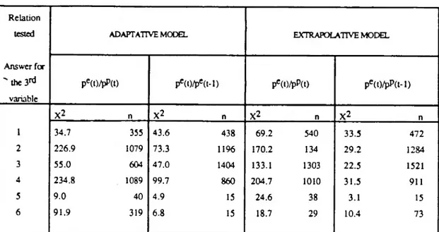
TABLE 1 : X2 test for the contingency tables (surveys 1987-1988).
Relation
tested ADAPTATIVE MODEL EXTRAPOLATIVE MODEL
Answer for
" the 3rd pe(t)/pP(t) pe(t)/pe(t-l) p'M/pPti) pe(t)/pP(t-l) variable X2 n X2 n X2 n X2 n 1 34.7 355 43.6 438 69.2 540 33.5 472 2 226.9 1079 73.3 1196 170.2 134 29.2 1284 3 55.0 604 47.0 1404 133.1 1303 22.5 1521 4 234.8 1089 99.7 860 204.7 1010 31.5 911 5 9.0 40 4.9 15 24.6 38 3.1 15 6 91.9 319 6.8 15 18.7 29 10.4 73 Remarks :
1) Adaptative model : pe(t) = flpe(t-l), pP(t)] Extrapolative model : pe(t) = g[pP(t-l), pP(t)]
When the relation between pe(t) and pP(t) is studied (for the adaptative model in the second column), the variable pe(t-l) is fixed at each of its six modalities (line one to six).
2) X2 calculated for the first four modalities of the two variables compared ; for five modalities, the X2 is, in the first column : 34.7, 257.7, 84.6, 243.1, 9.0, 91.9 ; the only clear difference between the X2 corresponding to 4 and 5 modalities appear in line 2, last column : X2 = 55.7 instead of 29.2.
3) n = number of households of the contengency table whose X2 is indicated (for 5 modalities - the fifth one being very rare).
4) X2 limit : 16.92 at 5 % ; 21.67 at 1 %.
One can conclude from table 1 :
(i) The X2 statistics are always significative : the contingency tables are thus proved to be asymétrie, and a direct observation of these tables shows that the relation existing between the two variables correspond to those which are predicted by the models (see Gardes-Madre, 1991, page 26).
(ii) The relations predicted by the adaptative model are better established than those of extrapolative model ( X2 greater of 16 % for the extrapolative model) : this result imports because it will be difficult to estimate the extrapolative model by the quantitative methods studied later.
(iii) The relation between past prices perceived in t and future prices expected in the same date (pP(t) and pe(t), corresponding to the adaptative and the regressive models), is more firmly established than the relation between expectations in (t-1) and t, or between past prices perceived in (t-1) and expectations made in t : thus, there appears a strong dependency between perceptions of past inflation and expectation made in the same period (L'Hardy, 1976, observed the same fact on macro data).
This qualitative analysis does not infirm the extrapolative and adaptative models. The quantification of the answers allows us to measure more precisely these relations.
SECTION 2 : QUANTIFICATION OF PERCEPTIONS AND EXPECTATIONS :
During the last twenty years, the inflation has been very changing in France : during a first period (1973-1983), prices have been increased by 10 % per year, with peaks at 15 % around 1974 and 1978 ; after a relatively short period of sharp decrease, inflation has remained around 3 % since 1985.
The modalities one to three of question five are labelled in levels for the perception of past inflation, while expectations (question 6) they are labelled in deviation to these perception of past inflation : this difference must be taken into account in the quantification.
Two types of measure have been performed.
2.1 First Quantification :
The more commonly used quantification of qualitative surveys consists in the definition of fixed hierarchised weights corresponding to each item of response, for instance an arithmetical scale from +2 to -2 when there are five modalities of response. These weights are added for the whole population to obtain an aggregate index : The often used Theil index, for instance (difference between the percentage of the first and the last modalities of response), consists in the scale +1,-1 for the extreme modalities and 0 for the other ones.
A fast mechanical quantification. Ia. is obtained through a scale +3 to -1 by attributing the nul weight to the modality 4 ("prices remain stationary") for question 5 on past perceived inflation, then adding 1, 0 or -1 to these perceived inflation rates according to the answer of the household to question 6 (acceleration, stability or decrease of inflation).
A second quantification, lb, is obtained by optimizing the choice of this scale through a minimisation of the difference between the actual inflation rate and the aggregate index calculated by the weighted sum of the percentages of answers .
To realize this optimization, aggregate data (the percentage of answers) have been used for the perception of past inflation, while individual data were used for the expectations. The details of this method are presented in Appendix II.
^ second type of quantification stays on the hypothesis of normal distributions of the responses to question 5 to 6. This method has been often used for aggregate data (for instance by de Menil, 1974 ; Carlson - Parkin, 1975 ; Prat, 1988, which presents it precisely pages 27-72) and we have adapted it to individual data : applied at a macro- level, the method affords the mean Ü of individual perceptions or expectations, and its standard error ^(see Appendix II for some detail) ; suppose that ai is the percentage of households having chosen the first modality for perceived past inflation, and si the threshold of a normal variable N(0,1) associated with the cumulate frequency ai/2, we quantify this first modality by the value IIP + si.s^/; for the second modality, the threshold S2 is associated to the cumulate frequency ai + a2/2 and this modality is quantify by the value np+ S2 S^pThe same quantification is applied to the qualitative expectation, but the choice of a mean expected inflation gives some trouble : it seems
natural to take, for each household, the value of the modality of past perceived inflation that he has declared, for question 6 is labelled in terms of "expectation compared to what is presently happening. In this first quantification (II a), we make in fact the hypothesis that the distribution of answers to question 6 does not depend on the modality chosen in question 5, for we use to determine the threshold si the distribution of the whole population on question 6. This independence of the two distributions corresponding to the question on past an future inflation is not proved by an empirical test, and, moreover, it gives rise to multicolinearity problems as piP(t) and pie(t) for household i will be related : pie(t) = piP(t) + si. .
A second hypothesis (quantification II b) consists to take the mean perceived past inflation IIP as the center of all expectations, and to define pie(t) = IIP + si ^ we lose the information on the dispersion of individual perceived past inflation, in addition to the information lost on the dispersion of individual expected inflation rates between the two thresholds of the modality of expectation chose by the household, but this second hypothesis gives rise to much better empirical results.
Other types of quantification are presented in Gardes-Madres (1991, page 32).
SECTION 3 : TEST OF RATIONALITY :
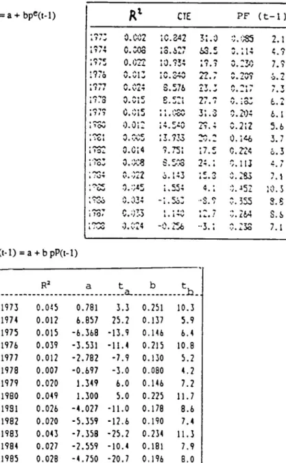
When the perceptions and expectations are aggregatedover all households4, unbiasedness and efficiency (against the perception of past inflation in (t-1) are positively tested, as shown by the following adjustments :
(1) (unbiasedness) pP(t) = 1.14 + 0.91 pc(t-l) ; R2 = 0.71 ; DW = 1.50 (0.61) (5.81)
(2) (efficiency) pP(t) - pe(t-l) = -0.11 pP(t-l) + 1.50 ; R2 = 0.03 ; DW = 1.46
(0.70) (0.73)
(annual data : 1973-1987 ; quantification II b).
As these agregate data follow a common trend (approximatively the trend of the actual inflation rate), these tests are not very convincing.
On the contrary, the expectations seem to be biased and unefficient on individual data, as table 1 and 2 show clearly : for the second quantification (II b), the coefficient of pc(t-l)
lies between 0.08 and 0.45, with a constant significantly different from 0 (and a weak R2, around 2 %) : a clear bias is shown. In equation (2), table 2, the perception of past inflation determines positively the errors of anticipation, with coefficients around + 0.2
and a mean R2 of 3 % : a weak unefficiency appears for the past perceptions of inflation.
Thus, one can conclude that tests of rationality on aggregate data are not significant, and that tests on individual data trend to prove some irrationality of expectations.
Table 1 : Unbiasedness : pP(t) = a + bpc(t-l) (quantification II b) Rl CTE PF (t-1) « 4 1 / V 0.C02 10.242 31.0 0.085 2.1 • « n tt o.cos • 40» Jt/A . A^ 63.5 0.114 4.7
\rz
0.022 • A AÏI 4 V» 7ÎT « A Al 7. 7 0.230 7.7 1?76 A A. •* V. « A A4 A4 V. ÛTTV 22.7 A AAAv. C.V7 6.2 4 lit A AA « V. Vit 3.576 ?T ▼ A A , -s V • - 4 / 7.3 • nirt 4 7.0 v.vuA As c £.521 27.7 A • A T V. ;Ov» 6.2 . ATA4 7/7 0.015 • « 4 4 . |\Aft'.OV 31.3 0.2i)4 6.1
1 toO 0.012 14.5*0 A»S « IT, *♦ 0.212 5.6 • aa « 4 <Gl A aOVJ,\C 13.733 <VS .V . •A 0.146 3.7 « 4 0.011 7.751 17.5 C. 224 6.3 4 AAT
i ’Ov o.oc« A CAA
c. ^.*o 24.1 0.11J i.7 . es»-» « 4 ;ot 0.022 o. 143 • C A iv. V 0. 2 S3 7.1 • a.tc . ' CaJ 0.045 1.554 4.1 0. -152 10.3 • (VS . 4 7 CO 0.034 “ 4 • 5o»j ..O o0. / 0.355 3. S i?o7 C. 03-3 1 • • A 4 . i 12.7 0.264 S. 6 . (WS 4 . '-O 0.024 -0.256 -•3.1 0.233 7.1
Table 2 : Efficiency : pP(t) - pe(t-l) = a + b pP(t-l) (quantification II b) R2 a t ...a_. b 1973 0.045 0.781 3.3 0.251 10.3 1974 0.012 6.857 25.2 0.137 5.9 1975 0.015 -6.368 -13.9 0.146 6.4 1976 0.039 -3.531 -11.4 0.215 10.8 1977 0.012 -2.782 -7.9 0.130 5.2 1978 0.007 -0.697 -3.0 0.080 4.2 1979 0.020 1.349 6.0 0.146 7.2 1980 0.049 1.300 5.0 0.225 11.7 1981 0.026 -4.027 -11.0 0.178 8.6 1982 0.020 -5.359 -12.6 0.190 7.4 1983 0.043 -7.358 -25.2 0.234 11.3 1984 0.027 -2.559 -10.4 0.181 7.9 1985 0.028 -4.750 -20.7 0.196 8.0 1986 0.018 -4.883 -32.3 0.147 6.4 1987 0.034 2.336 27.6 0.200 8.8 1988 0.036 0.194 2.2 0.210 8.8
SECTION 4 ; ESTIMATION OF MODELS OF ANTICIPATIONS :
3.1. Simple models :
The extrapolative model can be estimated, on an horizon of two years, by adjusting the expected inflation pe(t) on percepdon pP(t) and pP(t-l). For the first quantifications (la) and (lb), the measure of the expected inflation by adding an indicator of expectations to the perception of past inflation biases the estimation. The quantification II a (equivalent for this model to II b) allows us to observe (table 3) a positive correlation (R2 - 5,6 %), with a greater and more significant coefficient of pP(t) compared to pP(t-l) (0.11 against 0.03) ; it is interesting to note that the influence of these two past prices compensate one another from year to year : b = 0.85 c + 0.14 ; r2 = 17
(1.7)
past inflatign in t (pC(t)) being caracterized bv a greater coefficient when the inflation rate Changes rapidly (1975-1978 ; 1981 ; 1983-1987) : this fact proves that the anticipation does not follow a regular extrapolative process of past perceived evolutions, but that the weight given to these evolutions depends on the continuity or the ruptures of past evolutions.
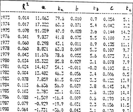
Table 3 : Extrapolative model : pe(t) = a + b pP(t-l) + cpP(t) (quantification II a) 197 IIJ o 0.014 0.017 3.078 « « A/ T i 1 . 'A^ IT TOO / • Oi— ti/35? K 79.0 63.3 0.010 0.071 0.0-23 0.054 0.042 A l V . i TT-1 A « n t • 17/Q 0.041 9.337 *t- CO 0.075 c c vJ . O 0.100 T -*/ • 1977 0.060 3.293 4 T 4 tv. 1 0.011 0.9 0.135 11.1 1973 0.060 3.821 63.3 0.049 C T J. N> 0.107 9.7 197? 0.043 11.676 73.6 0.C55 5. o /> at-t v. v/ 7.1 1930 0.034 15.322 33.3 0.029 3.1 0.073 7.9 1931 0.024 1* «IT It,Ti/ C * wTT. 41 -0.011 -0.3 0.103 o < U . 1 i IQl. 0.004 « T « rv-N l>>. TOz. •to. «g» / T 0.056 3.4 0.006 0.5 4 OAT
1 7 Q>j 0.073 tJ . O.tenj7 61.5 A AATV. VI./ T T sJ 0.122 13.9 « r-w-\ 4 1 7 Of A < 1 7V. i ig 6.636 56.0 0.03? y a v. 0 0.145 <1IT. ;0 • rw~vo 17 00 A « l vg A TQT / 0-.* AC «. 1 v • f> AT.vg 1 A i- . Û 0.120 t IT. T« • « r\o /
i 700 V. '.'GOA .NAO -1.5C? -It.4 A aaa
V. A Ot A V. i 7V• nn « « IT. A J 1937 A A To V* V# 7 -0.929 -19.9 A AT 4 V. ».»%/1 A T 0.156 11.51 • pnn 1700 v. VOTA A/ 4 _ « 1 • / V» 1TT « -36.0 0.043 T 4g. i
o
t >o
9.3 iThe regressive process can not be estimated without the definition of the reference inflation rate, corresponding to the long run equilibrium that the agents expect to be realized in the long term. If it is supposed constant, the model can be written : pc(t)-pP(t) = p [I! - pP(t)]. For the second quantification, the extrapolative equation corresponds to a coefficient p - 0.9 and an inflation rate n = constant/p which is not absurd. Nevertheless, a correct estimation would necessitate a better specification of the évolution of the long term inflation rate H
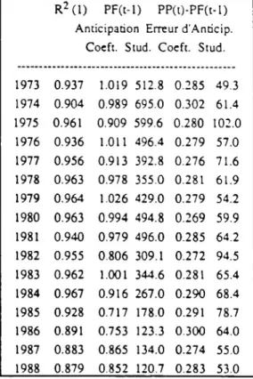
The simple adaptative model : pc(t) = (1-C)pe(t-1) + B pP(t) (3) = pc(t-l) + B EE(t) (4)
with an expectation error EE(t) = pP(t) - pe(t-l), has been estimated in the form (3) [with no constraint on the parameters], then by equation (4’) pe(t) - pc(t-l) = B EE(t) + $, with ^ supposed to be nul or not.
The first quantification (la) implies a mechanical effect (dpP=pP(t) - pP(t-l) being contained in each term of the equation) which fixes B around the unity ; the quantification lb (tables 4 and 5) gives rise on the contrary to a B around 0.3, the exceptional stability of which seems also due to a mechanical effect (proved by the excessive R2 for individual data).
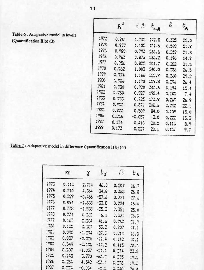
Table 4 : Adaptative model in levels (3) pe(t) = ( 1 -B)pe(t-1) + BpP(t) (Quantification lb)
R2 (1) PF(t-l) PP(t)-PF(t-l) Anticipation Erreur d'Anricip.
Coeft. Stud. Coeft. Stud.
1973 0.937 1.019 512.8 0.285 49.3 1974 0.904 0.989 695.0 0.302 61.4 1975 0.961 0.909 599.6 0.280 102.0 1976 0.936 1.011 496.4 0.279 57.0 1977 0.956 0.913 392.8 0.276 71.6 1978 0.963 0.978 355.0 0.281 61.9 1979 0.964 1.026 429.0 0.279 54.2 1980 0.963 0.994 494.8 0.269 59.9 1981 0.940 0.979 496.0 0.285 64.2 1982 0.955 0.806 309.1 0.272 94.5 1983 0.962 1.001 344.6 0.281 65.4 1984 0.967 0.916 267.0 0.290 68.4 1985 0.928 0.717 178.0 0.291 78.7 1986 0.891 0.753 123.3 0.300 64.0 1987 0.883 0.865 134.0 0.274 55.0 1988 0.879 0.852 120.7 0.283 53.0
(1) R2 du modèle avec terme constant.
Tabic 5 : Adaptative model in difference (4') dpc = B EE(t) + y
(Quantification lb)
Sources : Enquête INSEE de Conjoncture auprès des Ménages
The quantificatification (II a) gives also rise to a multicolinearity ; when corrected, B appears to be around 0.8 (when the equation contains also dpP in addition to EE(t). The quantification (II b) (tables 6 and 7) gives the better results : R2 around 18 %, and a B varying between 0.3 and 0.5, with significant and continuous variations from one year to another (0.2 to 0.4 for equation (3), 0.2 to 0.8 for (4’)) : the adjustment in level (equation (3)) verifies the additivity to one of the coefficients and shows that the inertia effect of pe(t-1 ) on pc(t) diminishes rapidly with the inflation rate after 1982 ; the adjustment in differences (equation (41)) shows that the influence of the expectation error EEiJÜ is paniçularlv important when the inflation rate is violently changed (1974-1975. ■1233, 198M986) and weak during the period of stability (1979-1982) : this correlation will be studied more thoroughly later.
R2 Constante Erreur d'Anticip. PP(t)-PF(t-l) Coeft. Stud. Coeft. Stud.
_______________* ft 1973 0.538 0.196 15.6 0.282 50.4 1974 0.573 -0.026 -2.6 0.299 60.3 1975 0.763 -0.439 -48.2 0.279 90.7 1976 0.557 0.156 12.8 0.277 57.9 1977 0.673 -0.352 -27.4 0.275 64.1 1978 0.620 0.012 0.9 0.282 61.1 1979 0.570 0.254 19.2 0.277 56.4 1980 0.583 0.049 4.1 0.267 59.8 1981 0.604 -0.051 -4.2 0.284 62.6 1982 0.674 -0.571 -47.9 0.273 73.4 1983 0.620 0.137 10.8 0.280 66.7 1984 0.625 -0.170 -11.7 0.280 60.1 1985 0.583 -0.454 -34.7 0.293 54.3 1986 0.555 -0.167 -13.1 0.306 50.6 1987 0.543 -0019 -1.7 0.270 49.4 1988 0.541 0.010 0.8 0.282 47.8
All these estimations of the adaptative model (summed in table 8) indicate a coefficient B bctyçgn Q,3 3nd 0,5. clearly less than the unity which is often obtained with aggregate data, (see Gardes-Madre, 1991, pages 49-50, for a discussion of this difference).
Table 6 : Adaptative model in levels (Quantification II b) (3)
10*r-r
A 7 / A V. >0lA/ « 1 AieA • A*Tw' * Art AA /
4fc 4 0 0.325 25.0 1974 A A*r*T V. ltt 4 4 00 A • 1 Ovf 131.6 {) V . J CAAl\J 51.9 « One .1/ ? A£V\ v* )Ov #\ AATU. / 7v 263.6 0.239 21.S * An/ ill o A A/TV, 70^. A AA ,V. 0/0 * OW. *. 0.196 14.9 1977 O AC"/ v* A Artrt V ■ Ü4-X AO « 4.V/1 • /«7 /N AAA v. aXu. A4 CXi 4 O a 7/0 0.962 4 AA7 Â • Wo AIO A A.TG. V C.336 A/ C4.0 . O 1979 0.974 4 111 A . loo 222.9 0.360 'VA A 1930 A / V. 7 00 4 4 Art A • 1 >0 259.3 A V. i.70Art I Oi A -.6. n 1981 A rtrtrt V/. 70V 0.920 *T J*T fOn*/, 0 0.194 *c ± iji a 1982 A AO A C.927 193.4 0.105 A « / 4 n 1 70 v I') Ocn V. • *>V» 0.725 « A / V. 7-r-r q 0.269 26.9 1984 A A«rn
V. 7^0 0.371 Artrt iA.VO. 0 A AIA
G, 22.1 1985 a rv>7 0.509 A 4 A O-t. 0 C. 159 15.0 1936 C.256 _ A AC—T v. Go/ A V. V 0.222 15.3 19S7 O « n a v« a/ n 0.410 20.5 0.113 £.9 1983 A 1 nn V* i / W 0.527 *Xy t4LV. 1 0.157 9.7
7 ■' Adaptative model in difference (quantification II b) (4')
R2 2 /3 t F, 4 n*r^ 17/j 0.113 ^ n< a.. / In« 46.0 0.207 16.7 4 A7# I 7 / «r 0.210 4.364 n 4 a on. 0 0.365 26.3 1975 0.229 -3.466 _e-7 / u/ t G 0.321 27.6 1976 0.094 4 * —A A.GoO -▼"* 0 *A/« V C.224 U A G • VL 4 A-»-» 17/ / 0.238 -1 Cf’O A • > W nc vOi A.a 0.351 AC 4.U. Va 4 A 70 1 7 / G V. f\ V. -w-Ai A 6.1 0.331 A, ■* 4 mo .7/7 V. AO/A 4 / A A AA 4«.t 4.vn n 4 4 a . 01 0.263. A4 A~A . 7 4 AOA
A 7O0 A « AC"V. AoO n 4 A*T
V. A v / C** A %rtw> • A A AAAV. OV/ 4 A 4A 7 • A 4 oo « 1 70 A V. A A AOv VO "A4 .*71AO 4 “•./ 4 VA O -4 V.Ain•> n4 4 4 4 0. Ü• A 4 rw\ A 7 0a. 0.037 “V. ÛA.0A AO l . « « 4 1 a. n A V. i n«.4 4 A 4 A 4A V. A 1 004 A VOv A V. T S.—T * O7 _▼ >>% iVO4 AC n/ .in a r> V'.llj« 4 c 38.3 4 A<*. 4
A 7 On A AAAM. 4.0 / _ 4 1 4 VO/HT1 A4 4on. n v. r* aa./ n-» 4 teV • vay q . AOC
• 7 uj A v. • • a noA V» n-»o / / V "O-v. ^* — A v. -.^Oatc « A 7 . *A A 4 AO i
1 /GO v. A 4 c 4a on 7.vn.4 T 4 A ..cn n«O»'. » V . ^ AAAA. / 0 4 A 4A 7 • V 4 rtrt^
A >0/ A AA4V. 4~on _f*» v • A-Von4 _#> ViWC •> V. VTV“• 4 A A4 on. -r4 4 rtrtrt
1 " OG A 4 V. A A 7n« _4 A 4 VJA/*C« _ • A 4 “ A 0. V Viviwa t.e A4 1 -A.G
Quantification n R2 la 0.68 0.90 lb 0.28 0.68 lia 0.84 0.08 lib* 0.28 0.18 lib** 0.52
-* En cl iff. première avec constante ** item sans constante
4.2 Mixed models :
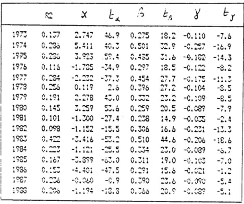
4.2.1. The introduction of the differential of past inflation perceived by the household (dpp) in the adaptative model :
dpe = a + 3 EE(t) + ÿ dpP (table 9)
shows a regressive behaviour of expectations, as y is clearly negative and 3 increases (to 0.35) compared to the simple adaptative model ; moreover, 3 and y seem to be negatively related, as if the regressive determinants appear when the adaptative ones lose their influence.
Table 9
'■ Regressive determinant in the adaptative model (quantification II b). ru. X t* /*> /oy
y! « n*rr• / / V r\ *V* AV/t 2.747 At OTV. 7 A 0. 4k/ ATCJ 4 0 AlUl 4.
-o.no
-7.6l7 / T a aa. V. 4.00 J.TilC « 4 4 TV 4 A • w*T A CA 1V 4 UV 1 32.9 "Vl A ACT 4k U/ -16.9 • rnc »■» ^ / V • 4. Où T .“VA"»
Of 71.0 . Ü *# . TCA « V.IOJA 4 -*C v;.oT 4 1 -0.132- 4 IT. O4 T
4a*71 17/6 0.116 _ 4 «7 AC 1 • / vV -34.9 0.2-97 1 A C1U. J -0.122 -0V. 4. ^ 4 C "7 "7 i 1 / / AA » v • 4kCrr _ A AT A *.« TT TV / 4 V 0.454 AT T 4./ • / -0.175 . « 1 1 4 V1 T 4 ATA 17/0
0.256
C) 1 * Q V. i i 7 A / -k.O0.396
AT A -k/ 4 4k-C. 104
_C* cV. V197?
r> 1Q1 v« A 7 A A AT A-.4.; o43.0
A VitwKJ-taa. AT A kVl X.-0.109
“S. 5
1930
A UCV, 1*TU T V. 4.J 7ACO C' / W. O A V. ij7ACO AA C4k V 4 V
A AAA “V. VO 7
-7.9
1931
0.101
-1.300
_ AT « 1./ • T0.238
14.9
—0.035
4.t T4 4 rv>A X 7 Oi.0.093
-1.152
-IP C!</• JC.3C6
16.6
-0.231
-13.3
1933
A « AA “i v. *tiO _CT A0.510
44.6
-0.206
-IE.6
4 nn< i 7(h A *4^7 "4 1•4 A41.1 AC C k.v. J0.334
23.0
-0.C3?
_ , T “ V 4 / * rvnc « 7 ÛJ V# 10/A 4 • T "• v. 077AAA _ : ■* UV 4 aV A T 1 4 V 4 V 1 119.0
-0V. 1 W *'ST / 4 f>V « aa/ i 700 A V • •* C-* *T 4 • TV 14 A 4 _ 4 t e t; • v cV C lo
15.6
A A A4 V. v.l ’l4.4 A « aa-» 170/ V. 4.^0at/-0.060
-0.9
0.390
4-V. OAT # - »'t '>£•*>V/ 4 V' / V _ C 4/4 **« < aaa 1700 A “VA »/ . -'/O# • 4 A 4 4 A A " i O. 0 A -i •V 4 VUU Art A -V . . _ »*. AAA “v.vO7 C 4V. 14.2.2. It is possible to mix systematically the three processes, as recommended by Frenkel, Curtin and Prat, by adding them with weights al, a2, a3 = l-ai*a2 to obtain the equation :
(5) pe(t) - pP(t) = (ai y - a3)dpP - a2 p pP(t) + a3 B[pP(t) - pc(t-l)] + a2 p
II
with three models :
- extrapolative (proportion ai) :
- regressive (a2) :
- adaptative (a3) :
pe(t)-pP(t) = ydpP
Pe(t) - pP(t) = pin - pP(t)]
(Al) pe(t) - pP(t) = -dpP + B EE(t) (A2) dpc = B EE(t)
When estimated separately, with pc(t) as the explained variable, the extrapolative process is badlv estimated (weak R2, around 5 %, constraint on the parameters not verified), while the regressive process is more precisely estimated (R2 «« 5,2 % ; p -0.89), and especially the adaptative process appears as the best estimated with a mean r2 of 7.6 %.
found in the previous analysis (4.2.1.) and badly estimated, the mixing of regressive and adaptative models shows, for the quantification lib, that (table 10) jj. a2 is close to 1 (0.7
in mean) : thus, as the regressivity coefficient fi is less than 1,
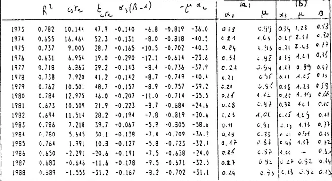
Table 10 : Mixed process regressive - adaptative
pe(t) - pP(t) = constant + a3(B-l) EE(t) - p a2 pP(t) (Quantification n b) R1 cj y*. t r -4) -c *u «*-1 fX TE7-43 1973 0.782 10.144 47.9 -0.140 -6.3 -0.819 -36.0 d a 1.21 c.)i 1974 0.655 16.464 52.3 -0.131 -8.0 -0.818 -40.5 e.M ■f.Cs o tr 7.11 1975 0.737 9.005 28.7 -0.165 -10.5 -0.702 -40.3 0.2 6 0.11 r 0 1976 0.631 6.954 19.0 -0.290 -12.1 -0.614 -23.6 c.ii i 52 a 15 -ft l oM 1977 0.718 6.863 29.2 -0.143 -8.4 -0.736 -37.9 C.2i t. tl 0.35 <5.0 1973 0.738 7.920 41.2 -0.142 -8.7 -0.749 -40.4 c il 0 ‘if d. l 1 -4.Cf C
1979 0.762 10.501 *8.7 -0.157 -8.9 -0.757 -39.2 iZt C/,5% Oil i4.ll » i‘3
1980 0.734 12.975 *6.0 -0.207 -11.0 -0.714 -35.5 o.il i.C- o.2c 4.
1981 0.673 10.509 21.9 -0.223 -8.7 -0.684 -24.6 U.tjj 0.8 7 0.31 4C 1 OAC 1982 0.694 11.514 28.2 -0.194 -7.9 -0.319 -30.6 :.l i A.CL c.if <6 0 C.ll 1983 0.786 7.213 39.7 -0.067 -5.9 -0.305 -58.6 6. Si 0 <1 4.K ••?> 1984 0.760 5.645 30.1 -0.133 -7.4 -0.709 -36.2 0.45 c.ss mi «04 Oil 1935 0.764 1.991 10.3 -0.127 -5.8 -0.723 -32.4 O.lr U C ^ 4.0 0. O 1936 0.650 -2.291 -20.6 -0.191 -7.5 -0.638 -24.0 c.lC C.ir 4 .cc - O.ki 1987 0.683 -0.646 -11.6 -0.178 -9.5 -0.671 -32.5 o.l > Cl ^ L v.Sl 0.1^
1938 0.639 -1.553 -31.2 -0.167 -3.2 -0.702 -31.1 02<i cii 1 C.ti v\ }
Hypothèses : (a)/3 = valeur obtenue dans le tableau 18
(b) 0 = valeur obtenue dans l’ajustement adaptatif en différence sans constante.
the regressive process appears to be influent (at> = 70 %) ; the coefficient B is estimated as clearly infra-unitary (if a3 is taken to be 30 %). If B = 0.28 for instance (as estimated separately in table 7), we obtain in mean p = 0.95 and a2 = 0.77, a3 = 0.23
The mix of these two processus is probably marked by the preponderance of one or the other in different periods, according as each household uses both processes (for instance for long term and short term expectations, as predicted by Frenkel, 1975) or as the proportion of households adopting each process varies. As an example of this phenomenon, we analyse the changes of the parameters of the adaptative process according to the level or to the volatility of inflation.
LEVEL OR THE VARIABILITY OF INFLATION
The volatility of inflation rates has been measured by different indicators of short-term volatility (s2, CV12, CV36) or long-term variability (s5, IdFIl) summing-up into the total variability 3 indicated by the standard-error of monthly inflation rates calculated on 36 months.
For the quantification (II b), strong correlations are observed between the annual coefficients B (estimated by equation (4')) of the expectation error and these indicators, the discordances with one type of variability (for example, the peak of 1974 or its variation after 1984, not correlated to the short-term indicators, being explained by the long-term ones).
The adjustments of B, for the period 1973-1988, on the level of the annual inflation rate, FI, its differential, dfl, and the variability indicators, show that :
(i) Thç total variability S~3 and the differential dfl (two variables with are not correlated! explain the two third of the variations of B :
/î = 93.5G3 + 35.0 dTf+ 0.05 ; R2 = 0.679. Dv/= 165 (2.51) (3.88) (0.56)
while the correlation of B with the level of inflation II is smaller :
/} = 78.4Cj + 13.47T+ constante ; R2 = 0.376, DW = 1.32 (1.20) (1.19)
(the correlation with the sole ^3 being already 31 %).
(ü) The influence of the total variability <P; preponderate fbv a factor 11 to 25) on that of fl and dfl. as is shown by the betas of these variables :
beta (53) = 43121 » bdia(r) = 1270 b<5ta (5-3) = 29293 » beta(dr) = 2652
components is not clear, even if these two components are positively correlated to B.
(iv) The annual differential of B is well explained by the differential and the variability of inflation :
dft= 35.5 dr+ 0.3 s5 - 0.05 : R2 = 0.44. DW = 1 77 (2.5) (1.4)
d/}= 45.0 dr+ 0.3 CV 12 - 0.08 ; R2 =0.44. DW = 194 (3.0) (1.4)
The same correlations exist between the quality of estimates (R2 and t of the estimations of equation (4')) and the variability of inflation (besides, B is correlated to the R2 of the adaptative equation : when the adaptative behaviour is strong, its become also rapid).
One can conclude that the annual estimations of the adaptative model, which are totally independent for the different years, indicate :
' that thç adaptative behaviour becomes more marked as the risk of the anticipation error increases (increased volatility or annual change of the inflation rate) ;
* a_myçh weaker relationship with the level of inflation contrary to what Cagan (1956) and Gibson (1972) have predicted: ^ = 44.4tr(l). 33.2irç,.|) + 0.I8 ; R2 = 0.59 DW = ,
(4-3) (3.0) (3.0)
Thus, these empirical results are rather a proof of the thesis proposed by Allais, Friedman - Schwartz (1982, page 358) and Tumovsky (1969) of a dependency of the antiçipatipn processes on the variability of the phenomenon anticipated. Besides, the variation of the coefficients of the adaptative model shows that its estimation on time series on a long period is biased by the hypothesis of the constancy of its parameters.
The analysis of INSEE panel data takes its interest on the presence of perceptions of past inflation as well as expectation of future inflation, and on the possibility to estimate expectation processes year per year, thus allowing to study the evolution of these processes and the causality of its evolution, and to test hypothesis made by Cagan, Gibson, Allais, Friedman Schwartz and Tumovsky.
New methods to quantify the quantitative data has been proposed, and it has been shown that traditional methods, imposing an a-priori scale for the hierarchised answers, give biased results.
Besides, on these individual data, the test of rationality and the estimates of inflation processes has been revealed as very different from the results obtained on aggregate data. The research will be continued to analyse the variation of the rationality properties and the expectations processes with the socio-economic characteristics of the households (some results already obtained are convergent with those published by Jonuung, 1980 (and Jonuung-Laidler, 1982), and to estimate on individual data the influence of anticipated and non-anticipated inflation on the households’ saving and consumption behaviour.
The French INSEE survey "Enquêtes de conjoncture auprès des ménages” (part of the European surveys) is made three times a year (October, January, May) on 6 000 to 8 000 households ; the October survey is renewed by half each year, so that about 2 500 households are interviewed in two consecutive years. Besides questions on socio economic caracteristics of the households, its equipment in durables, various expenses (holidays, purchase of cars and durables,...), it contains questions on the perception and anticipation of macro economic conditions (conjoncture, unemployment, inflation) and of the past and the future economic situation of the household.
6) General Questions :
1. Do you think that, for the last year, the level of being ("niveau de vie") of French people has :
1. been clearly improved ; 2. been a little improved ; 3. remained stationery ; 4. a little decreased ; 5. clearly decreased ; 6. do not know.
2. Do you think that, for the year to come, the level of being of French people will :
1. been clearly improved ; 2. been a Unie improved ; 3. remained stationery ; 4. a Unie decreased ; 5. clearly decreased ; 6. do not know.
market has during the previous months :
1. been clearly improved ; 2. been a little improved ; 3. remained stationery ; 4. a little decreased ; 5. clearly decreased ; 6. do not know.
4. Do you think that, for the months to come, the number of unemployed will :
1. been clearly improved ; 2. been a little improved ; 3. remained stationery ; 4. a little decreased ;
5. clearly decreased ;
6. do not know.
5. Do you feel that, since six months, the prices have :
1. much increased ; 2. meanly increased ; 3. A little increased ; 4. hardly varied ; 5. slightly decreased ; 6. do not know.
6. Compared to the present situation, do you think that for the next six months :
1. there will be a greater price increase ; 2. an equivalent price increase ;
3. a smaller price increase ; 4. prices will remain stationary ; 5. prices will slightly decrease ; 6. do not know.
The questions 7 to 17 concern the intentions to buy durable goods (especially cars) ; the perception of the past financial situation and the anticipation of the future one ; the intention to save and the type of saving wanted. These questions are analysed in Gardes- Madre (1989 ; Sept. 1990 ; January 1991) to test the consistency of households' expectations and the nullity of the transitory income elasticity of consumptions and savings.
APPENDIX n : QUANTIFICATION METHODS
1. Quantification Ih :
The quantification of the perception of past inflation has been performed on two distinct periods from : November 1974 to november 1983, from May 1984 to May 1989, the inflation rate being around 9 % during the first period and 3% during the second. The weights are determined by the adjustments of the semestrial serie of the actual inflation rate (p) on the percentages of each item of response : the first three give significant coefficients, but the weight attributed to the third modality ("little increase") is too close to
0 to be kept (the two other modalities are to rare to be considered) :
(a) November 1974-November 1983 : p = 3.0 12 + 7.8 Ij + 0.38 u(t-l) ; R2 = 0.52 5
(1.7) (9.1) (1.6) DW = 2.24
(b) May 1984-May 1989 : p = 1.8 12 + 6.7 Ij ; R2 = 0.898 ; DW = 1.98 (2-3) (6.4)
The weights are well hierarchised, but very different from the a-priori weights +2, +1, 0, -1,-2 which are commonly used, as in la.
The adjustments are not too different between the two periods, but we prefered to use seperate regressions because this method affords a better explanation of the period of désinflation (1983-1985).
In a second, the anticipation are quantified by minimizing on the whole panel (40 000 households) the distance between the individual expectations made in (t-1) and the perceived past inflation declared in t, pP(t) : this method consists in the minimization of the bias on the whole period, without imposing the absence of bias each year ; dummies has been introduced to take into account the variation of the inflation rate during the period, but the other coefficients have been shown not to vary much :
pP(t) = Constant + 0.268 pP(t-l) + 0.66 El + 0.48 E2 + 0.17 E3
(55.6) (12.4) (11.5) (3.6)
R2 = 0.796
where pP(t) and pP(t-l) are perceived inflation rates quantified previously (each household having the perceived inflation indicated by equations (a) and (b), for instance 3.0 for the first period and the households who chose the second response, if u(t-l) is nul) ; El, E2, E3 are dummies indicating the answers 1, 2, 3 to question 6, the fourth modality ("prices will remain stationary") being omited from the adjustment for multicolinearity reasons (the fifth modality is quite absent) and replaced a-priori by a 0. We note that the hierarchy of the coefficients is satisfied.
2. Quantification II :
Under the hypothesis of a normal distribution of answers one, can associate the threshold si to the proportion a 1 of households having chosen the first modality :
Proba
[Il
>si] = ai ; a second threshold s2 is associated to the population having chosen modalities 3, 4 and 5, talcing si = nn + S and S2 = Iln - 8, with nn a mean inflation late observed in the past, for the last n years (n = 1, 3, 5 in our estimations), and 8 a perception threshold fixed at 2 %.Taking Zi and Z2 as the thresholds of a normal reduced distribution corresponding to si and S2, the thresholds of the distribution N(n. of perception of past inflation or expectations, one obtains :
APPENDIX IU : Indicators of inflation volatility.
Short-term volatility has been measured by :
- CV12 = ratio of standart «Tor on mean of the monthly inflation rates, calculated over 12 months ;
- CV 36 = the same ratio calculated on 36 months ;
- s2 = ratio of the absolute difference on the mean of the monthly inflation rates.
Long-term volatility is measured by :
- S5 = ratio of the absolute difference between the annual inflation rate and its mean on the three last years, calculated over five years ;
- Idni = the absolute difference between two consecutive annual rates.
These two types of variability sum up into , the standart error of monthly rates, calculated on 36 months.
The correlations between these indicators is shown on the graph.
\ C vM £ C..CS o. b s £ ù<i,rl, m) z-o.l'i z W> /) -e
REFERENCES
CAGAN, P., 1956, The monetary dynamics of hyper inflation, in studies in the quantity theory of money, M. Friedman, ed., Chicago U.P.
CARLSON, .J.A., 1977, A study of price forecasts, Annals of Economic and social
measurement. January.
CHARPIN, F., 1988, Analyse rétrospective de l'enquête de conjoncture auprès des ménages,
Obser\’ations et Diagnostics économiques, n° 23, avril.
FANSTEN, M., 1976, Introduction à une théorie mathématique de l’opinion. Annales de
l'INSEE, n° 21, janvier-mars.
FRENKEL, J. A„ 1975, Inflation and the formation of expectations. Journal of Monetary Economies, vol. 1, 403-21.
FRIEDMAN, M, SCHWARTZ, A, 1982, Monetary Trends in the United States and United Kingdom, University of Chicago Press.
GARDES,F., 1990a, Une procédure de révélation des anticipations de revenu et de prix. Cahier du GRID, mai.
GARDES, F., 1990b, Income and price expectations in the irish and French consumption and saving functions, Kilkenny, 18 mai, Annual meeting of the Irish Economic Association,
Cahiers du GRID, mai.
GARDES, F., MADRE J.L., 1989, Achats d’automobiles et anticipations des ménaees.
rapport CREDOC.
GARDES, F., MADRE J.L., 1989, Achats d’automobiles et anticipations des ménages, 6ème journées de Microéconomies Appliquées, Orléans, mai
GARDES, F. MADRE J.L., 1990d, Modèles d’anticipation des prix : comparaison des estimations sur données macroéconomiques et microéconomiques en France, 7ème Journées de Microéconomie Appliquée, Montréal, mai.
GARDES, F. MADRE J.L., 1990b, Les anticipations de revenu et de prix dans les enquêtes INSEE de conjoncture auprès des ménages. Troisième colloque international sur les données de panel, ENSAE, 12 juin.
GARDES, F. MADRE J.I.., 1990, Consumption and transitory income ; an estimation on a panel of French data. Economics Letters, September.
GIBSON, \V„ 1972. Interest rates and inflationary expectations : new evidence, American
Economic Review, december.
GLAUDE, M„ 1981, La réalisation des intentions d'achat. Economie et Statistique, janvier.
I,'HARDY, P-- 1976, Les attitudes des ménages : leur signification. Economie et Statistique, janvier.
PESARAN, M.H., 1987. The limits to rational expectations. Blackwell.
PRAT, G., 1988, Analyse des anticipations d’inflation des ménages : France et Etats-Unis.
Economica.
STERDYNIAK, H., 1988, Opinions, anticipations et consommation des ménages.
Observations et diagnostics économiques, n° 23, avril.
TURNOVSKY, SJ., 1969, A Bayesian approach to the theory of expectations. Journal of
RëCHERCHE
Récemment parus
s;i3îi'«^éSî!KssS: -;-r-r r"T\ ‘ *gkéf&i y:-ï r;~*::,T - -h • I ffiÉSSÉ ySi»|àS; ÿ"-4 il iljfefc ; ‘-W-X-5t=5?î -' " ■■'■-[^1 *■— iwîlife.wI-... - 'prima: i'ïïÿS
. • ■ -■- --- H
• =i: ■i :•-•<•■•••
r r,
-: ; -.4 V -:• . . .
I
Penser l'insertion - Méthodes et critères : Contribution à une analyse des critères de l’insertion dans les réseaux de prise en charge des jeunes en difficulté, par Michel Legros, N° 14, Avril 1991.
L'analyse propositionnelle du discours, par Michel Messu, N° 15, Mai 1991.
Classification dichotomique descendante par Sébastien Lion, N° 16, Mai 1991.
Pratiques exemplaires ou exemples de pratiques : l’évaluation dans le secteur social aux Etats-Unis - Analyse de monographies présentées dans "Evaluation Review" et dans "Evaluation and the health professions", par Patricia Croutte, Michel Legros, N° 17, Juillet 1991.
Etude de l'opinion et enquêtes de référence : Aspects théoriques, méthodologiques et informatiques (Soutenance : Avril 1988), par Anastassios Iliakopoulos, N° 18, Septembre 1991.
Entre école et emploi : les transitions incertaines, par Denise Bauer, Patrick Dubéchot, Michel Legros, N ° 19, Septembre 1991.