CONDITIONED-U-NET: INTRODUCING A CONTROL MECHANISM IN THE U-NET FOR MULTIPLE SOURCE SEPARATIONS

HAL Id: hal-02448917

https://hal.archives-ouvertes.fr/hal-02448917

Submitted on 22 Jan 2020

HAL is a multi-disciplinary open access

archive for the deposit and dissemination of

sci-entific research documents, whether they are

pub-lished or not. The documents may come from

teaching and research institutions in France or

abroad, or from public or private research centers.

L’archive ouverte pluridisciplinaire HAL, est

destinée au dépôt et à la diffusion de documents

scientifiques de niveau recherche, publiés ou non,

émanant des établissements d’enseignement et de

recherche français ou étrangers, des laboratoires

publics ou privés.

CONDITIONED-U-NET: INTRODUCING A

CONTROL MECHANISM IN THE U-NET FOR

MULTIPLE SOURCE SEPARATIONS

Gabriel Meseguer-Brocal, Geoffroy Peeters

To cite this version:

Gabriel Meseguer-Brocal, Geoffroy Peeters.

CONDITIONED-U-NET: INTRODUCING A

CON-TROL MECHANISM IN THE U-NET FOR MULTIPLE SOURCE SEPARATIONS. Proceedings of

the 20th International Society for Music Information Retrieval Conference, Nov 2019, Delft,

Nether-lands. �10.5281/zenodo.3527766�. �hal-02448917�

CONDITIONED-U-NET: INTRODUCING A CONTROL MECHANISM IN

THE U-NET FOR MULTIPLE SOURCE SEPARATIONS

Gabriel Meseguer-Brocal

Ircam Lab, CNRS, Sorbonne Universit´e 75004 Paris, France

gabriel.meseguerbrocal@ircam.fr

Geoffroy Peeters

LTCI, T´el´ecom Paris, Institut Polytechnique de Paris, 75013, Paris, France

geoffroy.peeters@telecom-paris.fr

ABSTRACT

Data-driven models for audio source separation such as U-Net or Wave-U-Net are usually models dedicated to and specifically trained for a single task, e.g. a particu-lar instrument isolation. Training them for various tasks at once commonly results in worse performances than train-ing them for a strain-ingle specialized task. In this work, we introduce the Conditioned-U-Net (C-U-Net) which adds a control mechanism to the standard U-Net. The control mechanism allows us to train a unique and generic U-Net to perform the separation of various instruments. The C-U-Net decides the instrument to isolate according to a one-hot-encoding input vector. The input vector is embedded to obtain the parameters that control Feature-wise Linear Modulation (FiLM) layers. FiLM layers modify the U-Net feature maps in order to separate the desired instrument via affine transformations. The C-U-Net performs different in-strument separations, all with a single model achieving the same performances as the dedicated ones at a lower cost.

1. INTRODUCTION

Generally, in Music Information Retrieval (MIR) we de-velop dedicated systems for specific tasks. Facing new (but similar) tasks require the development of new (but similar) specific systems. This is the case of data-driven music source separation systems. Source separation aims to isolate the different instruments that appear in an au-dio mixture (a mixed music track) i.e., reversing the mix-ing process. Data-driven methods use supervised learnmix-ing where the mixture signals and the isolated instruments are available for training. The usual approach is to build dedi-cated models for each task to isolate [1, 20]. This has been proved to show great results. However, since isolating an instrument requires a specific system, we can easily run into problems such as scaling issues (100 instruments = 100 systems). Besides, these models do not use the com-monalities between instruments. If we modify them to do

© Gabriel Meseguer-Brocal, Geoffroy Peeters. Licensed under a Creative Commons Attribution 4.0 International License (CC BY 4.0). Attribution: Gabriel Meseguer-Brocal, Geoffroy Peeters. “Conditioned-U-Net: introducing a control mechanism in the U-Net for multiple source separations”, 20th International Society for Music Infor-mation Retrieval Conference, Delft, The Netherlands, 2019.

Figure 1: [Left part] Traditional approach: a dedicated U-Net is trained to separate a specific source. [Right part] Our proposition based on conditioning learning. The prob-lem is divided in two: a standard U-Net (which provides generic source separation filters) and a control mechanism. This division allows the same model to deal with different tasks using the commonalities between them.

various tasks at once i.e., adding fix numbers of output masks in last layers, they reduce their performance [20].

Conditioning learning has appeared as a solution to problems that need the integration of multiple resources of information. Concretely, when we want to process one in the context of another i.e., modulating a system com-putation by the presence of external data. Conditioning learning divides problems into two elements: a generic system and a control mechanism that governs it according to external data. Although there is a large diversity of do-mains that use it, it has been developed mainly in the image processing field for tasks such as visual reasoning or style transfer. There, it has been proved very effective, improv-ing the state of the art results [4, 14, 21]. This paradigm can be integrated into source separation creating a generic model that adapts to isolate a particular instrument via a control mechanism. We also believe that this paradigm can benefit to a great diversity of MIR tasks such as multi-pitch estimation, music transcription or music generation.

In this work, we propose the application of condition-ing learncondition-ing for music source separation. Our system relies on a standard U-Net system not specialized in a specific task but rather in finding a set of generic source separation filters, that we control differently for isolating a particular instrument, as illustrated in Figure 1. Our system takes as input the spectrogram of the mixed audio signal and the control vector. It gives as output (only one) the separated instrument defined by the control vector. The main advan-tages of our approach are - direct use of commonalities between different instruments, - a constant number of pa-rameters no matter how many instruments the system is dealing with - and scalable architecture, in the sense that

new instruments can be potentially added without training from scratch a new system. Our key contributions are:

1. the Conditioned-U-Net (C-U-Net), a joint model that changes its behavior depending on external data and performs for any task as good as a dedicated model trained for it. C-U-Net has a fixed number of parameters no matter the number of output sources. 2. The C-U-Net proves that conditioning learning (via

Feature-wise Linear Modulation (FiLM) layers) is an efficient way of inserting external information to MIR problems.

3. A new FiLM layer that works as good as the original one but with a lower cost (fewer parameters).

2. RELATED WORK

We review only works related to conditioning in audio and to data-driven source separation methods.

Conditioning in audio. It has been mainly explored in speech generation. In the WaveNet approach [23, 24] the speaker identity is fed to a conditional distribution adding a learnable bias to the gated activation units. A WaveNet modified version is presented in [19]. The time-domain waveform generation is conditioned by a sequence of Mel spectrogram computed from an input character sequence (using a recurrent sequence-to-sequence network with at-tention). In speech recognition conditions are used in [11], applying conditional normalisation to a deep bidirec-tional LSTM (Long Short Term Memory) for dynamically generating the parameters in the normalisation layer. This model adapts itself to different acoustic scenarios. In [11], the conditions do not come from any external source but rather from utterance information of the model itself. They have been also used in music generation for accompani-ments conditioned on melodies [7] or incorporating history information (melody and chords) from previous measures in a generative adversarial network (GAN) [26]. Finally, it has been also proved to be very efficient for piano tran-scription [6]: the pitch onset detection is internally con-catenated to the frame-wise pitch prediction controlling if a new pitch starts or not. Both, onset detection and frame-wise prediction are trained together.

Source separation based on supervised learning. We refer the reader to [16] for an extensive overview of the different source separation techniques. We review only the data-driven approaches. Here, the neural networks have taken the lead. Although architectures such as RNN [8] or CNN [2] have been studied, the most successful one use a deep U-Net architecture (also called U-Net). In [1], the U-Net is applied to a spectrogram to separate the vocal and accompaniment components, training a specific model for each task. Since the output is the spectrogram, they need to reconstruct the audio signal which potentially leads to ar-tifacts. For this reason, Wave-U-Net proposes to apply the U-Net to the audio-waveform [20]. They also adapt their model for isolating different sources at once by adding to

Figure 2: [Top part] FiLM simple layer applies the same affine transformation to all the input feature maps x. [Bot-tom part] In the FiLM complex layer, independent affine transformations are applied to each feature map c.

their dedicated version as many outputs as sources to sep-arate. However, this multi-instruments version performs worse than the dedicated one (for vocal isolation) and has to be retrained to different source combinations.

The closest work to ours is [10]. In there, they propose to use multi-channel audio as input to a Variational Auto-Encoder (VAE) to separate 4 different speakers. The VAE is conditioned on the ID of the speaker to be separated. The proposed method outperforms its baseline.

3. CONDITIONING LEARNING METHODOLOGY 3.1 Conditioning mechanism.

There are many ways to condition a network (see [5] for a wide overview) but most of them can be formalized as affine transformations denoted by the acronym FiLM (Feature-wise Linear Modulation) [14]. FiLM permits to modulate any neural network architecture inserting one or several FiLM layers at any depth of the original model. A FiLM layer conditions the network computation by apply-ing an affine transformation to intermediate features:

F iLM (x) = γ(z) · x + β(z) (1) where x is the input of the FiLM layer (i.e., the interme-diate feature we want to modify), γ and β are parameters to be learned. They scale and shift x based on the external information, z. The output of a FiLM layer has the same dimension as the intermediate feature input x. FiLM layers can be inserted at any depth i in the controlled network.

As described in Figure 2, the original FiLM layer ap-plies an independent affine transformation to each feature map c1_{: γ}

i,c and βi,c [14]. We call this a FiLM complex

layer (Co). We propose a simpler version that applies the same γi and βi to all the feature maps (therefore γ and β

do not depend on c). We call it a FiLM simple layer (Si). The FiLM simple layer decreases the degrees of freedom of the transformations to be carried out forcing them to be generic and less specialized. It also reduces drastically the number of parameters to be trained. As FiLM layers do not change the shape of x, FiLM is transparent and can be used in any particular architecture providing flexibility to the network by adding a control mechanism.

3.2 Conditioning architecture.

A conditioning architecture has two components:

The conditioned network. It is the network that carries out the core computation and obtains the final output. It is usu-ally a generic network that we want to behave differently according to external data. Its behavior is altered by the condition parameters, γi,(c)and βi,(c)via FiLM layers.

The control mechanism - condition generator. It is the system that produces the parameters (γ’s and β’s) for the FiLM layers with respect to the external information z: the input conditions. It codifies the task at hand and provides the instructions to control the conditioned network. The condition generator can be trained jointly [14, 21] or sepa-rately with the conditioned network [4].

This paradigm clearly separates the tasks description and control instructions from the main core computation.

4. CONDITIONED-U-NET FOR MULTITASK SOURCE SEPARATION

We formalize source separation as a multi-tasks problem where one task corresponds to the isolation of one in-strument. We assume that while the tasks are different they share many similarities, hence they will benefit from a conditioned architecture. We name our approach the Conditioned-U-Net (C-U-net). It differs from the previ-ous works where a dedicated model is trained for a single task [1] or where it has a fixed number of outputs [20].

As in [1, 20], our conditioned network is a standard U-Net that computes a set of generic source separation filters that we use to separate the various instruments. It adapts itself through the control mechanism (the condition gen-erator) with FiLM layers inserted at different depths. Our external data is a condition vector z (a one-hot-encoding) which specify the instrument to be separated. For exam-ple, z = [0, 1, 0, 0] corresponds to the drums. The vector z is the input to the control mechanism/condition genera-tor that has to learn the best γi,cand βi,cvalues such that,

when they modify the feature maps (in the FiLM layers) the C-U-Net separates the indicated instrument i.e., it de-cides which features maps information is useful to get each instrument. The control mechanism/condition generator is itself a neural network that embeds z into the best γi,cand

βi,c. The conditioned network and the condition generator

are trained jointly. A diagram is shown in Figure3. Our C-U-Net can perform different instrument source separations as it alters its behavior depending on the value of the external condition vector z. The inputs of our system are the mixture and the vector z. There is only one output, which corresponds to the isolated instrument defined by z. While training, the output corresponds to the desired isolated instrument that matches the z activation.

4.1 Conditioned network: U-Net architecture

We used the U-Net architecture proposed for vocal separa-tion [1], which is an adaptasepara-tion of the microscopic images

Figure 3: The C-U-Net has two distinct parts: the condi-tion generator and a standard U-Net. The former codifies the input the condition vector, z (with the instrument to iso-late) for getting the needed γi,(c) and βi,(c). The generic

U-Net has as input the magnitude spectrum. It adapts its conduct via FiLM layers inserted in the encoder part. The system outputs the desired instrument defined by z.

U-Net [18]. The input and output are magnitude spectro-grams of the monophonic mixture and the instrument to isolate. The U-Net follows an encoder-decoder architec-ture and adds a skip connection to it.

Encoder. It creates a compressed and deep representation of the input by reducing its dimensionality while preserving the relevant information for the separation. It consists of a stack of convolutional layers, where each layer halves the size of the input but doubles the number of channels. Decoder. It reconstructs and interprets the deep features and

transforms it into the final spectrogram. It consists of a stack of deconvolutional layers.

Skip-connections. As the encoder and decoder are sym-metric i.e., feature maps at the same depth have the same shape, the U-Net adds skip-connections between layers of the encoder and decoder of the same depth. This refines the reconstruction by progressively providing finer-grained information from the encoder to the decoder. Namely, fea-ture maps of a layer in the encoder are concatenated to the equivalent ones in the decoder.

The final layer is a soft mask (sigmoid function ∈ [0, 1]) f (X, θ) which is applied to the input X to get the isolated source Y . The loss of the U-Net is defined as:

L(X, Y ; θ) = kf (X, θ)  X − Y k1,1 (2)

where θ are the parameters of the system.

Architecture details. Our implementation mimics the original one [1]. The encoder consists in 6 encoder blocks. Each one is made of a 2D convolution with 5x5 filters, stride 2, batch normalisation, and leaky rectified linear

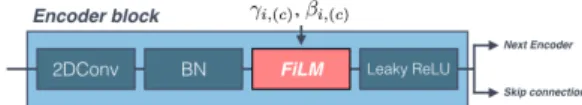
Figure 4: FiLM layers are placed after the batch normal-isation. The output of a encoding block is connected to both, the next encoding block and the equivalent layer in the decoder via the skip connections.

units (ReLU) with leakiness 0.2. The first layer has 16 fil-ters and we double them for each new block. The decoder maps the encoder, with 6 decoders blocks with stride de-convolution, stride 2 and a 5x5 kernel, batch normalisation, plain ReLU, and a 50% dropout in the first three. The final one, the soft mask, uses a sigmoid activation. The model is trained using the ADAM optimiser [12] and a 0.001 learn-ing rate. As in [1], we downsample to 8192 Hz, compute the Short Time Fourier Transform with a window size of 1024 and hop length of 768 frames. The input is a patch of 128 frames (roughly 11 seconds) from the normalised (per song to [0, 1]) magnitude spectrogram for both the mixture spectrogram and the isolated instrument.

Inserting FiLM. The U-Net has two well differenti-ated stages: the encoder and decoder. The enconder is the part that transforms the mixture magnitude input into a deep representation capturing the key elements to isolate an instrument. The decoder interprets this representation for reconstructing the final audio. We hypothesise that, if we can have a different way of encoding each instrument i.e., obtaining different deep representations, we can use a common ‘universal’ decoder to interpret all of them. Fol-lowing this reasoning, we decided to condition only the U-Net encoder part. In the C-U-U-Net, a FiLM layer is inserted inside each encoding block after the batch normalisation and before the Leaky ReLU, as described in Figure 4. This decision relies on previous works where feature are modi-fied after the normalisation [4,11,14]. Batch normalisation normalises each feature map so that it has zero mean and unit variance [9]. Applying FiLM after batch normalisa-tion re-scale and re-shift feature maps after the activanormalisa-tions. This allows the net to specialise itself to different tasks. As the output of our encoding blocks is transformed by the FiLM layer the data that flows through the skip con-nections carries on also the transformations. If we use the FiLM complex layer, the control mechanism/condition generator needs to generate 2016 parameters (1008 γi,c

and 1008 βi,c). On the other hand, FiLM simple layers

imply 12 parameters: one γiand one βifor each of the 6

different encoding blocks, which means 2002 parameters less than for FiLM complex layers.

4.2 Condition generator: Embedding nets

The control mechanism/condition generator computes the γi,(c)(z) and βi,(c)(z) that modify our standard U-net

be-havior. Its architecture has to be flexible and robust to gen-erate the best possible parameters. It has also to be able to find relationships between instruments. That is to say, we want it to produce similar γi,(c) and βi,(c) for instruments

Table 1: Params number in millions. With dedicated U-Nets, each task needs a model with 10M params. C-U-Nets are multi-task and the number of params remains constant.

MODEL Non-conditioned SiF CoF SiC CoC

PARAM 39,30 (4 tasks x 9,825) 9,85 12 9,84 10,42

that have similar spectrogram characteristics. Hence, we explore two different embeddings: a fully connected ver-sion and a convolutional one (CNN). Each one is adapted for the FiLM complex layer as well as for the FiLM sim-ple layer. In every control mechanism/condition genera-tor configuration, the last layer is always two concatenated fully connected layers. Each one has as many parameters (γ’s or β’s) as needed. With this distinction we can control γi,(c)and βi,(c)individually (different activations).

Fully-Connected embedding (F): it is formed of a first dense layer of 16 neurons and two fully connected blocks (dense layer, 50% dropout and batch normalization) with 64 and 256 neurons for FiLM simple and 256 and 1024 for FiLM complex. All the neurons have relu activations. The last fully connected block is connected with the final con-trol mechanism/condition generator layer i.e., the two fully connected ones (γi,cand βi,c). We call the C-U-Net that

uses these architectures C-U-Net-SiF and C-U-Net-CoF. CNN embedding (C): similarly to the previous one and

in-spired by [19], this embedding consists in a 1D convolution with lenght(z) filters followed by two convolution blocks (1D convolution with also lenght(z) filters, 50% dropout and batch normalization). The first two convolutions have ‘same’ padding and the last one, ‘valid’. Activations are also relu. The number of filters are 16, 32 and 64 for the FiLM simpleversion and 32, 64, 256 for the FiLM com-plexone. Again, the last CNN block is connected with the two fully connected ones. The C-U-Net that uses these architectures are called C-U-Net-SiC and C-U-Net-CoC. This embedding is specially designed for dealing with sev-eral instruments because it seems more appropriated to find common γi,(c)and βi,(c)values for similar instruments.

The various control mechanisms only introduce a re-duced number of parameters to the standard U-Net archi-tecture remaining constant regardless of the instruments to separate, Table 1. Additionally, they make direct use of the commonalities between instruments.

5. EVALUATION

Our objective is to prove that conditioned learning via FiLM (generic model+control) allows us to transform the U-Net into a multi-task system without losing perfor-mances. In Section 5.1 we review our experiment design aspects and we detail the experiment to validate the multi-task capability of the C-U-Net in Section 5.2.

5.1 Evaluation protocol

Dataset. We use the Musdb18 dataset [17]. It consists of 150 tracks with a defined split of 100 tracks for training

Table 2: Overall performance (mean ± std) for the 4 tasks. Si= simple FiLM, Co= complex FiLM, F= Fully-embed and C= CNN-embed, p= progressive train or np= not.

MODEL Total SIR SAR SDR Fix-U-Net(x4) 7.31 ± 4.04 5.70 ± 3.10 2.36 ± 3.96 C-U-Net-SiC-np 7.35 ± 4.13 5.74 ± 3.18 2.34 ± 3.69 C-U-Net-SiC-p 8.00 ± 4.37 5.74 ± 3.63 2.54 ± 4.07 C-U-Net-CoC-np 7.27 ± 4.24 5.60 ± 2.88 2.36 ± 3.81 C-U-Net-CoC-p 7.49 ± 4.54 5.67 ± 3.03 2.42 ± 4.21 C-U-Net-SiF-np 7.23 ± 3.97 5.59 ± 3.01 2.22 ± 3.67 C-U-Net-SiF-p 7.64 ± 4.05 5.73 ± 2.88 2.46 ± 3.88 C-U-Net-CoF-np 7.42 ± 4.20 5.59 ± 3.07 2.32 ± 3.85 C-U-Net-CoF-p 7.52 ± 4.04 5.71 ± 2.99 2.42 ± 3.97

and 50 for testing. From the 100 tracks, we use 95 (ran-domly assigned) for training, and the remaining 5 for the validation set, which is used for early stopping. The per-formance is evaluated on the 50 test tracks. In Musdb18, mixtures are divided into four different sources: Vocals, Bass, Drums and Rest of instruments. The ’Rest’ task mixes every instrument that it is not vocal, bass or drums. Consequently, the C-U-Net is trained for four tasks (one task per instrument) and z has four elements.

Evaluation metrics. We evaluate the performances of the separation using the mir evaltoolbox [15]. We com-pute three metrics: Source-to-Interference Ratios (SIR), Source-to-Artifact Ratios (SAR) and Source-to-Distortion Ratios (SDR) [25]. To compute the three measure we also need the predicted ’accompaniment’ (the mixture part that does not correspond to the target source). Each task has a different accompaniment e.g., for the drums the accom-paniment is rest+vocals+bass. We create the accompani-ments by adding the audio signal of the needed sources. Audio Reconstruction method. The system works

exclu-sively on the magnitude of audio spectrograms. The output magnitude is obtained by applying the mask to the mix-ture magnitude. As in [1], the final predicted source (the isolated audio signal) is reconstructed concatenating tem-porally (without overlap) the output magnitude spectrums and using the original mix phase unaltered. We compute the predicted accompaniment subtracting the predicted iso-lated signal to the original mixture. Despite there are better phase reconstruction techniques such as [13], errors due to this step are common to both methods (U-Net and C-U-Net) and do not affect our main goal: to validate condi-tioning learning for source separation.

Activation function for γ and β. One of the most impor-tant design choices is the activation function for γi,(c) and

βi,(c). We tested all the possible combinations of three

acti-vation functions (linear, sigmoid and tanh) in the C-U-Net-SiF configuration. As in [14], the C-U-Net works better when γi,(c) and βi,(c) are linear. Hence, our γ’s and β’s

have always linear activations.

Training flexibility. The conditioning mechanism gives the flexibility to have continuous values in the input z ∈ [0, 1],

Table 3: Task comparison between the dedicated U-Nets and the C-U-Net-CoF. Results indicate that they perform similarly for all the tasks. We also add the multi-instrument Wave-U-Net (M) results (median in parenthesis) and when possible the dedicated version (D). For vocals isolation the Wave-U-Net-M performs worse than the Wave-U-Net-D.

Model SIR SAR SDR

V ocals Fix-U-Net(x4) 10.70 ± 4.26 5.39 ± 3.58 3.52 ± 4.88 (4.72) C-U-Net-CoF 10.76 ± 4.39 5.32 ± 3.27 3.50 ± 4.37 (4.65) Wave-U-Net-D - - 0.55 ± 13.67 (4.58) Wave-U-Net-M - - -2.10 ± 15.41 (3.0) Drums Fix-U-Net(x4) 10.08 ± 4.28 6.42 ± 3.28 4.28 ± 3.65 (4.13) C-U-Net-CoF 10.03 ± 4.34 6.80 ± 3.25 4.30 ± 3.81 (4.38) Wave-U-Net-M - - 2.88 ± 7.68 (4.15) Bass Fix-U-Net(x4) 4.64 ± 4.76 6.51 ± 2.68 1.46 ± 4.31 (2.48) C-U-Net-CoF 5.30 ± 4.73 6.29 ± 2.39 1.65 ± 4.07 (2.60) Wave-U-Net-M - - -0.30 ± 13.50 (2.91) Rest Fix-U-Net(x4) 3.83 ± 2.84 4.47 ± 2.85 0.19 ± 3.00 (0.97) C-U-Net-CoF 4.00 ± 2.70 4.37 ± 3.06 0.24 ± 3.64 (1.71) Wave-U-Net-M - - 1.68 ± 6.14 (2.03)

which weights the target output Y by the same value. We call this training method progressive. In practice, while training, we randomly weight z and Y by a value between 0 and 1 every 5 instances. This is a way of dealing with ab-lations by making the control mechanism robust to noise. As shown in Table 2, this training procedure (p) improves the models. Thus, we adopt it in our training. More-over, preliminary results (not reported) show that the C-U-Net can be trained for complex tasks like bass+drums or voice+drums. These complex tasks could benefit from ‘in between-class learning’ method [22] where z will have different intermediate instrument combinations.

5.2 Multitask experiment

We want to prove that a given C-U-Net can isolate the Vo-cals, Drums, Bass, and Rest as good as four dedicated U-Net trained specifically for each task2 We call this set of dedicated U-Nets, Fix-U-Nets. Each C-U-Nets version (one model) is compared with the Fix-U-Nets set (four models). We review the results at Table 2 and show a com-parison per task in Table 3.

Results in Table 2 for all 4 instruments highlight that FiLM simple layers work as good as the complex ones. This is quite interesting because it means that applying 6 affine transformations with just 12 scalars (6 γiand 6 βi)

at a precise point allows the C-U-Net to do several source separations. With FiLM complex layers it is intuitive to think that treating each feature map individually let the C-U-Net learn several deep representations in the encoder. However, we have no intuitive explanation for FiLM sim-plelayers. We did the Tukey test with no significant dif-ferences between the Fix-U-Nets and the C-U-Nets for any task and metric. Another remark is that the four C-U-Nets benefit from the progressive training. Nevertheless, it im-pacts more the simple layers than in the complex ones. We think that the restriction of the former (fewer parameters) helps them to find an optimal state.

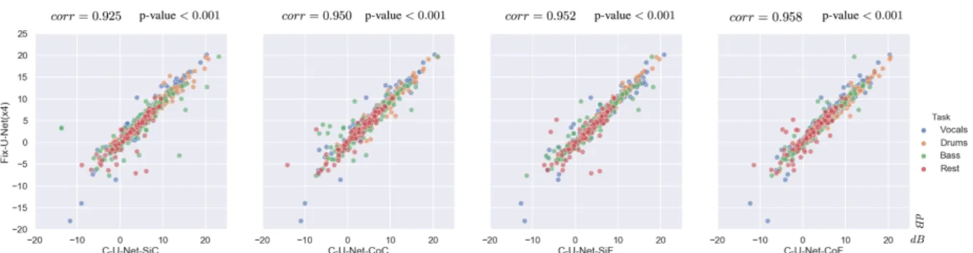
Figure 5: Each graph correlates the performance of two models. On top of it, we show the correlation and p-value. The ’y’ axis represents the fixed version (the four dedicated U-Nets) and the ’x’ one a different C-U-Net version (with progressive train). The coordinates of each dots correspond to the models’ performance i.e., ’y’ position for the Fix-U-Net performance and ’x’ for C-U-Net. There are three dots per song one per metric (SIR, SAR, and SDR) which does a total of 600 (50 songs x 3 metrics x 4 instruments). The dots alignment in the diagonal implies a strong correlation between models: if one works well, the others too and vice versa. Each color highlights the points of each source separation task.

However, these results do not prove nor discard the significant similarity between systems. For demonstrat-ing that we have carried out a Pearson correlation exper-iment. The results are detailed in Figure 5. The Pearson coefficient measures the linear relationship between two sets of results (+1 implies an exact linear relationship). It also computes the p-value that indicates the probability that uncorrelated systems have produces them. Our dis-tinct C-U-Net configurations have a global corr > .9 and p-value < 0.001. Which means that there is always more than 90% correlation between the performance of the four dedicated U-Nets and the (various) conditional version(s). Additionally, there is almost no probability that a C-U-Net version is not correlated with the dedicated ones. We have also computed the Pearson coefficient and p-value per task and per metric with the same results. In Figure 5 shows a strong correlation between the Fix-U-Net results and the distinct C-U-Nets (independently of the task or metric). Thus, if one works well, the others too and vice versa.

In Table 3 we detail the results per task and metric for the Fix-U-Net and the C-U-Net-CoF which is not the best C-U-Net but the one with the highest correlation with the dedicated ones. There we can see how their performances are almost identical. Nevertheless, our vocal isolation (in any case) is not as good as the one reported in [1], we believe that this is mainly due to the lack of data. These results can only be compared with the Wave-U-Net [20]. Although they report the results (only the SDR) for the four tasks in the multi-instrument version (multiple outputs layers) they only have a dedicated version for vocals. For vocal separation, the performance of the multi-instrument version decreases more than 2.5 dB in mean, 1.5 dB in the median and the std increase in almost 2 dB. Furthermore, the C-U-Net performs better than the multi-instrument in three out of four tasks (vocals, bass, and drums)3_{. For the}

’Rest’ task, the multi-instrument wave-u-net outperforms our C-U-Nets. This is normal because the dedicated U-Net

3_{Our experiment conditions are different in training data size (95 Vs}

75) and in sampling rate (8192 Hz Vs 22050 Hz) than Wave-U-Net.

has already problems with this class and the C-U-Nets in-herits the same issues. We believe that they come from the vague definition of this class with many different instru-ments combinations at once.

This proves that the various C-U-Nets behave in the same way as the dedicated U-Nets for each task and metric. It also demonstrates that conditioned learning via FiLM is robust to diverse control mechanisms/condition generators and FiLM layers. Moreover, it does not introduce any lim-itations which are due to other factors.

6. CONCLUSIONS AND FUTURE WORK We have applied conditioning learning to the problem of instrument source separations by adding a control mecha-nism to the U-Net architecture. The C-U-Nets can do sev-eral source separation tasks without losing performance as it does not introduce any limitation and makes use of the commonalities of the distinct instruments. It has a fixed number of parameters (much lower than the dedicated ap-proach) independently of the number of instruments to sep-arate. Finally, we showed that progressive training im-proves the C-U-Nets and introduced the FiLM simple, a new conditioning layer that works as good as the original one but requires less γ’s and β’s.

Conditioning learning faces problems providing a generic model and a control mechanism. This gives flex-ibility to the systems but introduces new challenges. We plan to extend the C-U-Net to more instruments to find its limitations and to explore the performance for com-plex tasks i.e., separating several instruments combinations (e.g., vocals+drums). Likewise, we are exploring ways of adding new conditions (namely new instrument isolation) to a trained C-U-Net and how to detach the joint training. We also intend to integrate it other architectures such as Wave-U-Net and data augmentation techniques [3].

Lastly, we believe that conditioning learning via FiLM will benefit many MIR problems because it defines a trans-parent and direct way of inserting external data to modify the behavior of a network.

Acknowledgement. This research has received funding from the French National Research Agency under the contract ANR-16-CE23-0017-01 (WASABI project). Implementation and audio examples available at https://github.com/gabolsgabs/cunet

7. REFERENCES

[1] N. Montecchio R. Bittner A. Kumar T. Weyde A. Jansson, E. J. Humphrey. Singing voice separation with deep u-net con-volutional networks. In Proc. of ISMIR (International Society for Music Information Retrieval), Suzhou, China, 2017. [2] P. Chandna, M. Miron, J. Janer, and E. G´omez.

Monoau-ral audio source separation using deep convolutional neuMonoau-ral networks. In Proc. of LVA/ICA (International Conference on Latent Variable Analysis and Signal Separation), Grenoble, France, 2017.

[3] Alice Cohen-Hadria, Axel Roebel, and Geoffroy Peeters. Im-proving singing voice separation using deep u-net and wave-u-net with data augmentation. CoRR, abs/1903.01415, 2019. [4] H. de Vries, F. Strub, J. Mary, H. Larochelle, O. Pietquin, and A. C. Courville. Modulating early visual processing by lan-guage. In Proc. of NIPS (Annual Conference on Neural Infor-mation Processing Systems), Long Beach, CA, USA, 2017. [5] V. Dumoulin, E. Perez, N. Schucher, F. Strub, H. de Vries,

Aaron Courville, and Y. Bengio. Feature-wise transfor-mations. Distill, 2018. https://distill.pub/2018/feature-wise-transformations.

[6] C. Hawthorne, E. Elsen, J. Song, A. Roberts, I. Simon, C. Raffel, J. Engel, S. Oore, and D. Eck. Onsets and frames: Dual-objective piano transcription. In Proc. of ISMIR (In-ternational Society for Music Information Retrieval), Paris, France, 2018.

[7] C. A. Huang, A. Vaswani, J. Uszkoreit, N. Shazeer, C. Hawthorne, A. M. Dai, M. D. Hoffman, and D. Eck. An improved relative self-attention mechanism for transformer with application to music generation. CoRR, abs/1809.04281, 2018.

[8] Po-Sen Huang, Minje Kim, Mark Hasegawa-Johnson, and Paris Smaragdis. Joint optimization of masks and deep re-current neural networks for monaural source separation. IEEE/ACM TASLP (Transactions on Audio Speech and Lan-guage Processing), 23(12), 2015.

[9] Sergey Ioffe and Christian Szegedy. Batch normalization: Accelerating deep network training by reducing internal co-variate shift. In Proc. of ICML (International Conference on Machine Learning), 2015.

[10] H. Kameoka, Li Li, S. Inoue, and S. Makino. Semi-blind source separation with multichannel variational autoencoder. CoRR, abs/1808.00892, 2018.

[11] T. Kim, I. Song, and Y. Bengio. Dynamic layer normalization for adaptive neural acoustic modeling in speech recognition. CoRR, abs/1707.06065, 2017.

[12] Diederik P. Kingma and Jimmy Ba. Adam: A method for stochastic optimization. In Proc. of ICLR (International Con-ference on Learning Representations), Banff, Canada, 2014. [13] F. Mayer, D. Williamson, P. Mowlaee, and D. Wang.

Im-pact of phase estimation on single-channel speech separation based on time-frequency masking. The Journal of the Acous-tical Society of America, 141:4668–4679, 2017.

[14] E. Perez, F. Strub, H. de Vries, V. Dumoulin, and A. C. Courville. Film: Visual reasoning with a general condition-ing layer. In Proc. of AAAI (Conference on Artificial Intelli-gence), New Orleans, LA, USA, 2018.

[15] C. Raffel, B. Mcfee, E. J. Humphrey, J. Salamon, O. Nieto, D. Liang, and D. P. W. Ellis. mir eval: a transparent imple-mentation of common mir metrics. In Proc. of ISMIR (In-ternational Society for Music Information Retrieval), Porto, Portugal, 2014.

[16] Z. Rafii, A. Liutkus, F.-R. St¨oter, S. Ioannis Mimilakis, D. Fitzgerald, and B. Pardo. An Overview of Lead and Accompaniment Separation in Music. IEEE/ACM TASLP (Transactions on Audio Speech and Language Processing), 26(8), 2018.

[17] Zafar Rafii, Antoine Liutkus, Fabian-Robert St¨oter, Stylianos Ioannis Mimilakis, and Rachel Bittner. The MUSDB18 corpus for music separation, 2017. https://zenodo.org/record/1117372.

[18] O. Ronneberger, P. Fischer, and T. Brox. U-net: Convolu-tional networks for biomedical image segmentation. In Proc. of MICCAI (International Conference on Medical Image Computing and Computer Assisted Intervention), Munich, Germany, 2015.

[19] J. Shen, R. Pang, R. J. Weiss, M. Schuster, N. Jaitly, Z. Yang, Z. Chen, Y. Zhang, Y. Wang, R. J. Skerry-Ryan, R. A. Saurous, Y. Agiomyrgiannakis, and Y. Wu. Natural TTS synthesis by conditioning wavenet on mel spectrogram pre-dictions. In Proc. of ICASSP (International Conference on Acoustics, Speech and Signal Processing), Calgary, Canada, 2018.

[20] D. Stoller, S. Ewert, and S. Dixon. Wave-u-net: A multi-scale neural network for end-to-end audio source separation. In Proc. of ISMIR (International Society for Music Informa-tion Retrieval), Paris, France, 2018.

[21] F. Strub, M. Seurin, E. Perez, H. de Vries, J. Mary, P. Preux, A. C. Courville, and O. Pietquin. Visual reasoning with multi-hop feature modulation. In Proc. of ECCV (European Confer-ence on Computer Vision), Munich, Germany, 2018. [22] Y. Tokozume, Y. Ushiku, and T. Harada. Between-class

learn-ing for image classification. In Proc. of CVPR (Conference on Computer Vision and Pattern Recognition), Salt Lake City, UT, USA, 2018.

[23] A. van den Oord, S. Dieleman, H. Zen, K. Simonyan, O. Vinyals, A. Graves, N. Kalchbrenner, A. W. Senior, and K. Kavukcuoglu. Wavenet: A generative model for raw au-dio. CoRR, abs/1609.03499, 2016.

[24] A. van den Oord, Y. Li, I. Babuschkin, K. Simonyan, O. Vinyals, K. Kavukcuoglu, G. van den Driessche, E. Lock-hart, L. C. Cobo, F. Stimberg, N. Casagrande, D. Grewe, S. Noury, S. Dieleman, E. Elsen, N. Kalchbrenner, H. Zen, A. Graves, H. King, T. Walters, D. Belov, and D. Hassabis. Parallel wavenet: Fast high-fidelity speech synthesis. CoRR, abs/1711.10433, 2017.

[25] E. Vincent, R. Gribonval, and C. F´evotte. Performance mea-surement in blind audio source separation. IEEE/ACM TASLP (Transactions on Audio Speech and Language Processing), 14(4), 2006.

[26] Li-Chia Yang, Szu-Yu Chou, and Yi-Hsuan Yang. Midinet: A convolutional generative adversarial network for symbolic-domain music generation using 1d and 2d conditions. CoRR, abs/1703.10847, 2017.