Développement d'un nouveau concept de test de réponse thermo-hydraulique pour échangeurs de chaleur géothermiques verticaux

i

DÉVELOPPEMENT D’UN NOUVEAU CONCEPT DE

TEST DE RÉPONSE THERMO-HYDRAULIQUE

POUR ÉCHANGEURS DE CHALEUR

GÉOTHERMIQUES VERTICAUX

Mémoire

JEAN ROULEAU

MAÎTRISE EN GÉNIE MÉCANIQUE Maître ès sciences (M.Sc.)

Québec, Canada

iii

Résumé

Il est important de connaître la conductivité thermique du sol ainsi que l’amplitude et l’orientation de la vitesse des écoulements souterrains lors du dimensionnement d’un champ de puits géothermiques. Ce mémoire présente la méthodologie et les conclusions d’une analyse numérique d’un nouveau concept de test de réponse thermique (TRT) pour échangeurs de chaleur géothermiques verticaux. Cette configuration de TRT permet de mesurer à la fois les propriétés hydrauliques du sol et ses propriétés thermiques. Le but premier du mémoire est de vérifier la validité du concept pour ensuite développer une méthode de résolution permettant d’estimer, à partir de la réponse thermique lors du TRT, la conductivité thermique du sol ainsi que la norme et l’orientation de la vitesse des écoulements souterrains. Pour ce faire un modèle numérique de puits a été construit avec la méthode des éléments finis afin d’effectuer des simulations numériques de la réponse thermique dans diverses conditions. À partir de ces simulations, il a été possible de démontrer le potentiel du concept de TRT et d’élaborer des méthodologies pour retrouver les propriétés désirées. Une méthode de résolution graphique est d’abord présentée. Dans un second temps, le formalisme des problèmes inverses est appliqué afin d’obtenir une deuxième méthode de mesure des paramètres du sol. Les résultats montrent que le TRT proposé permet de retrouver ces paramètres dans la plupart des scénarios envisagés.

v

Abstract

It is important to know the subsurface thermal conductivity and the groundwater flow parameters (i.e. its velocity and orientation) when sizing a geothermal borefield. This master’s thesis presents a methodology and the conclusions of a numerical analysis of a novel thermal response test (TRT) concept for vertical geothermal heat exchangers. This configuration of TRT is able to measure both the hydraulic and the thermal properties of the ground. The main objective behind this work is to validate the concept and then to develop an efficient methodology to obtain from the thermal response of the TRT an estimation of the ground thermal conductivity along with the velocity and the orientation of groundwater flows. To achieve this, a numerical model of borehole was built using the finite element method. This model was then used to simulate the thermal response for various conditions. From these simulations, it has been possible to demonstrate the potential of the concept and to elaborate methodologies to find the desired properties. A graphical method is first presented. Following that, inverse problem techniques were applied to get a second measurement methodology. Results show that the suggested TRT is able to find the parameters in most of the cases.

vii

Table des matières

Résumé ... iii

Abstract ...v

Liste des tableaux ... ix

Liste des figures ... xi

Nomenclature ... xiii Remerciements ... xvii Avant-Propos ... xix Chapitre 1 Introduction ...1 1.1 Problématique ...1 1.2 Objectifs ...3 1.2.1 Objectif principal ...3 1.2.2 Objectifs secondaires ...3

1.3 Méthode et présentation du document ...3

1.3.1 Chapitre 2 – Nouveau concept de test de réponse combinée hydro-thermique pour échangeurs de chaleur géothermique ...4

1.3.2 Chapitre 3 – Emploi de concepts de résolution de problème de transfert thermique inverse pour la mesure des propriétés hydro-thermiques du sol ...5

Chapitre 2 Article de revue ...7

Résumé ...8

Abstract ...9

2.1 Introduction ... 10

2.2 Description of the concept ... 12

2.3 Mathematical and numerical models... 13

2.3.1 Governing equations ... 15

2.3.2 Numerical model ... 18

2.4 Influence of groundwater flow during H/TRT ... 19

2.5 Proposed methodology for H/TRT analysis ... 23

2.5.1 Evaluation of the groundwater flow orientation ... 23

2.5.2 Evaluation of groundwater flow velocity ... 25

2.5.3 Evaluation of thermal conductivity ... 28

2.5.3.1 Time needed for the temperature in the borehole to be uniform ... 28

2.5.3.2 Ground function for various Pe and ... 29

2.5.4 Schematic step-by-step analysis procedure ... 31

2.6 Conclusions ... 37

Chapitre 3 Article de revue ... 39

Résumé ... 40

Abstract ... 41

3.1 Introduction ... 42

viii

3.2 H/TRT Modeling ... 44

3.2.1 H/TRT set-up ... 44

3.2.2 Governing equations ... 45

3.2.3 Numerical model ... 48

3.3 Inverse heat transfer approach ... 49

3.3.1 Error function ... 49

3.3.2 Error minimization iterative procedure ... 50

3.3.3 Sensitivity analysis ... 51

3.3.3.1 Ratio of volumetric heat capacities ... 51

3.3.3.2 Ratio of thermal conductivities ... 51

3.3.3.3 Peclet number ... 52

3.3.3.4 Flow orientation ... 53

3.3.4 Parameter estimation strategy ... 54

3.4 Impacts of initial guess ... 56

3.4.1 Influence of flow orientation uncertainty ... 56

3.4.2 Influence of the initial guess for conductivity and Peclet number ... 58

3.5 Performance of the estimation methodology ... 60

3.6 Conclusions ... 66

Chapitre 4 Conclusion ... 69

ix

Liste des tableaux

Table 2.1: Typical groundwater Darcy velocity in various geological materials. 14

Table 2.2 : Properties of water for the numerical model. 14

Table 2.3 : Simulated range for all variables. 17

Table 2.4 : Direction calculated after a day of heating for different groundwater velocities 24 Table 2.5: Error on the extrapolation of the maximal difference of temperature according to the accuracy

of the flow orientation measurement . 26

Table 2.6: Values for parameters A0 and A1 as a function of conductivity and Peclet number. 29 Table 2.7: Test case used for evaluation of required borefield length as a

function of the ground parameters. 36

Table 3.1: Solution of the inverse heat transfer problem using different numbers of parameters in a single

optimization. 55

Table 3.2: Evaluation of the ratio of thermal conductivities and the groundwater flow Peclet number for

multiple initial guesses. 59

Table 3.3: Effective thermal conductivity calculated from the line source method for different flow

velocities. 65

xi

Liste des figures

Fig. 2.1 Schematic representation of the proposed H/TRT setup with groundwater flow. 12 Fig. 2.2: Mesh of the numerical model used for simulation of the proposed H/TRT setup

with groundwater flow 19

Fig. 2.3: Example of simulated temperature profile in and around the borehole after a day of heating. 20 Fig. 2.4: Example of temperature evolution measured by sensors for a) Pe=0.001 b) Pe=0.01

c) Pe=0.05 and d) Pe=0.1. 21

Fig. 2.5: Example of the evolution of the differences of temperature between sensors for a) Pe=0.001

b) Pe=0.01 c) Pe=0.05 and d) Pe=0.1. 22

Fig. 2.6: Schematic view of the borehole during the test to illustrate the definition of T_max. 25 Fig. 2.7: Maximum dimensionless difference of temperatures on the borehole wall

versus the flow Peclet number. 27

Fig. 2.8: Ground function for the TRT a) as a function of the Peclet number, and b) as a function of the

ratio of thermal conductivities. 31

Fig. 2.9: Suggested flowchart for the H/TRT analysis procedure. 33

Fig. 2.10: Comparison between estimates of the parameters obtained from the H/TRT and their actual values for a series of random cases: a) subsurface thermal conductivity b) Darcy velocity

c) flow orientation d) required borefield length 35

Fig. 3.1: Schematic representation of the modified H/TRT set-up to measure

the ground thermal and hydraulic properties 44

Fig. 3.2: Influence of k on the objective function for different Peclet numbers, with  90. 52

Fig. 3.3: Influences of Pe on the objective function for different flow orientations, with k = 4 . 53 Fig. 3.4: Error on the estimated flow orientation according to the Peclet number. 57 Fig. 3.5: Effects of an error on the estimation of  on the measurement of: a) k, and b) Pe. 58 Fig. 3.6: Comparison of the estimated parameters to the real ones for: a) subsurface thermal

conductivity, b) Darcy velocity, and c) the required borefield length. 62 Fig. 3.7: Comparison of the error on the required total GHE length by the H/TRT apparatus with the one

xiii

Nomenclature

Lettres latines

A0, A1 Paramètres de corrélation

B Distance entre deux puits, m cp Capacité thermique, J/kg K CF Facteur de correction f Champ vectoriel Fo Nombre de Fourier G Fonction caractéristique k Conductivité thermique, W/mK M Nombre de capteurs de température N Nombre de puits

P Pression, Pa

P Vecteur de paramètres inconnus Pe Nombre de Péclet

q Taux de transfert de chaleur du puits, W

0

q



_{Taux d’injection de chaleur de la source, W/m}

R Résistance thermique, mK/W r Coordonnée radiale, m

S Norme des moindres carrées, _{K ×s}2 t Temps, s

T Température, K, °C u Vitesse, m/s

x,y Coordonnées cartésiennes, m Y Température mesurée, K, °C

Lettres grecques

α Diffusivité thermique, m2_/s

 Perméabilité du sol, m2

xiv



_{Densité, kg/m}3



Porosité du sol



_{Ratio des capacités thermiques volumétriques}  Température relative TTg, K, °C

 Orientation de l’écoulement, °

 Temps d’un pulse, heure, mois, année  Variable aléatoires

 Écart standard des erreurs de mesure, K, °C Indices avg Moyen b Puits c Critique calc Calculée cs Capteur rapproché D Darcy eff Effective ex Exact f Fluide fs Capteur éloigné g Sol non-dérangé H Grande

h Pulse par heure Heat Période de chauffage i Intérieur L Petite M Milieu m Pulse mensuel Max Maximum o Extérieur p Position de mesure

xv

s Solide

test Test de réponse thermo-hydraulique true Vrai U Uniforme y Pulse annuel 0 Initial Symboles ~ Non-dimensionnel



Vecteur  Moyenné

xvii

Remerciements

Ce mémoire n’aurait jamais été possible sans l’aide de plusieurs personnes qui ont su contribuer de diverses manières. Je tiens à profiter de cet espace pour souligner leur contribution et les remercier.

Un incontournable est mon directeur de recherche, Louis Gosselin. Son apport a été essentiel à l’achèvement de cet ouvrage. Lorsque j’étais dans une impasse, il n’a jamais hésité à agir tel un guide pointant la bonne direction en plus de faire preuve de patience et de grande disponibilité. Louis est un passionné de la recherche, de la science et de la vie en général et je dois bien admettre qu’il m’a transmis cette passion. Je considère que c’est un privilège de pouvoir travailler avec un professeur aussi exceptionnel.

Mes remerciements suivant vont à tous mes collègues du Laboratoire de Transfert

Thermique et d’Énergétique (LTTE). Durant ces années, j’étais entouré jour après jour

d’une équipe dynamique formant une ambiance de travail fort agréable. Je tiens à remercier personnellement Maxime Tye-Gingras pour m’avoir enseigné les notions d’éléments finis nécessaires au démarrage de mon projet de recherche. Pour Ruijie Zhao, 谢谢 pour les divers trucs que tu m’as montrés lors de mon apprentissage du chinois! Merci à Alexandre, François, Jean-Michel, Jonathan, Maarten, Mathieu, Maxime, Noémie, Raphael, Richard, Ruijie et à tous les autres.

Mes derniers remerciements sont pour ma famille. D’abord, mes parents, Yves et Ginette, et ma sœur Marie-Josée, qui m’ont tous apporté un soutien financier, culinaire mais surtout moral pendant tout ce temps. Sans leur éducation et leur présence, je n’aurais sans doute jamais atteint ce point, autant d’un point de vue académique que personnel. Mes dernières lignes sont dédiées à ma marraine Sylvie et mon parrain Serge. Malgré les terribles défis qu’ils ont vécus, leur jovialité demeurerait toujours une source de motivation pour moi. À Sylvie, je dis : Lâche pas la patate!

xix

Avant-Propos

Les deux articles présentés dans ce mémoire ont été coécrits par l’auteur de ce mémoire, Jean Rouleau, et son directeur de recherche, Louis Gosselin. Jean Rouleau, soit l’auteur principal de ces textes, a réalisé les recherches, l’élaboration du modèle numérique utilisé, les simulations numériques, l’analyse des résultats ainsi que la majorité de la rédaction des articles. Le second co-auteur, Louis Gosselin, fut le superviseur de ces travaux en guidant l’étudiant tout au long de ses recherches en plus d’aider à la rédaction et la correction des documents présentés. Le premier article a été co-écrit également par le professeur Jasmin Raymond, de l’INRS-ÉTÉ, qui a apporté son regard d’hydrogéologue lors de l’élaboration de l’article. Ces articles sont pour le moment soumis. Afin d’améliorer leur cohérence dans ce mémoire, quelques modifications mineures, telle que la numérotation des tableaux et figures et celle des références bibliographiques, ont étés apportées à leur version originale.

1

Chapitre 1 Introduction

1.1 Problématique

L’énergie géothermique représente l’énergie contenue sous forme de chaleur dans le sol. La présence de cette chaleur est due à la fois à la désintégration d’éléments radioactifs dans l’écorce terrestre et à la chaleur originale emprisonnée au cœur de la terre lors de sa formation. Une fois soutirée du sol par transferts thermiques, cette énergie peut servir divers secteurs : production d’électricité, chauffage et climatisation de bâtiments, chauffage de l’eau (autant pour les bains et piscines que pour la pisciculture), etc. Étant donné le faible gradient géothermique que l’on retrouve sur la plupart du territoire canadien, la géothermie au Canada a pour principale application de fournir de l’énergie à un système de pompe à chaleur, qui est autant en mesure de chauffer les bâtiments en hiver que de les climatiser en été. On dénote tout de même un certain potentiel de production d’électricité géothermique au Québec [1][2].

Bien que plus que négligeable avant les années 1990, le marché géothermique canadien est en impressionnante progression depuis les deux dernières décennies [3][4]. Le Canada ne fait pas bande à part puisqu’une tendance similaire est observable sur l’ensemble de la planète [5]. De par sa nature écologique, la géothermie cadre bien avec le développement durable et la protection de l’environnement. Toutefois, malgré cet intérêt croissant pour l’énergie du sol, cette technologie fait toujours face à des défis tels que la réduction des coûts de forage et le dimensionnement plus efficace des puits.

2

Un de ces défis est la difficulté de mesurer efficacement les propriétés du sol à une profondeur de l’ordre du 100 mètres. Pour concevoir un bon design d’un champ de puits géothermiques, il est essentiel de connaitre les propriétés du sol où on souhaite le construire. La conductivité thermique du sol est évaluée à partir d’une opération que l’on nomme test de réponse thermique (TRT). Cependant, bien que des études ont montré que la conductivité thermique est la propriété qui influence le plus la performance d’un échangeur géothermique, de plus en plus d’études indiquent également que les propriétés hydrauliques peuvent avoir une grande importance [6][7]. Par conséquent, de plus en plus de modèles de champs géothermiques requièrent la connaissance de la vitesse et de l’orientation de l’écoulement de l’eau contenu à l’intérieur des aquifères [8], puisque cet écoulement a un effet sur le transfert thermique se produisant entre les puits et le sol [9][10]. Les essais hydrogéologiques effectués [11][12] pour mesurer les écoulements souterrains sont coûteux en termes d’argent et de temps, et ne sont à toutes fins pratiques jamais utilisés pour des applications comme la géothermie. De leur côté, les tests de réponse thermique actuels ne considèrent pas ces écoulements souterrains; ils sont généralement basés sur une hypothèse d’échange de chaleur purement par conduction dans le sol [13]. Le fait d’ignorer le mouvement de l’eau peut induire, à moyen ou long terme, une erreur sur la performance réelle d’un champ géothermique par rapport à celle attendue. Il serait donc bénéfique de concevoir un test pouvant combiner l’aspect hydrogéologique à l'aspect thermique. L’étude présentée dans ce mémoire se consacre ainsi à l’établissement et la validation d’un nouveau concept de test de réponse thermique qui permettrait cette combinaison. Une telle implantation permettrait des économies d’argent, d’équipement, de main-d’œuvre et de temps.

3

1.2 Objectifs

1.2.1 Objectif principal

Ce projet de recherche a pour objectif principal de valider un nouveau concept de test de réponse thermo-hydraulique. Trois principaux points d’amélioration sont ainsi ciblés dans le projet : (1) Pouvoir estimer avec justesse la conductivité thermique du sol malgré l’influence des écoulements souterrains; (2) Mesurer les caractéristiques de l’écoulement hydrogéologique en même temps que les propriétés thermiques du sol et (3) Réduire les dépenses reliées au TRT.

1.2.2 Objectifs secondaires

 Concevoir un modèle numérique par éléments finis d’un puits vertical soumis à un écoulement hydrogéologique. Des simulations examinant le nouveau concept de TRT pourront y être produites.

 À partir des résultats obtenus par les simulations, bâtir une méthode d’analyse simple permettant de déterminer la conductivité thermique du sol en plus de la vitesse et de l’orientation de l’écoulement d’eau qu’il contient.

1.3 Méthode et présentation du document

Le montage suggéré de test de réponse thermique a dû être validé par une étude numérique, ce qui demande la modélisation numérique d’un domaine représentant un puits dans un sol où de l’eau s’écoule. La qualité première désirée pour ce modèle numérique était la rapidité à effectuer une simulation puisque ce modèle devait être utilisé à maintes reprises au cours de l’étude. Le modèle bâti est bidimensionnel pour cette raison. Le fait d’ignorer la dimension verticale requiert certaines hypothèses qui ont été jugées comme étant acceptables. Ce modèle a servi à la mise en place d’une méthode de résolution donnant les variables désirées selon la réponse thermique du montage. Deux méthodes distinctes offrent cette possibilité : une méthode graphique et une numérique, qui emploie des

4

principes de problème inverse de transfert de chaleur. Les deux ont été développées dans le cadre de ce travail.

Le mémoire a un format par articles; il est principalement constitué de deux articles scientifiques rédigés par l’auteur. Ces deux articles sont présentement soumis à des journaux scientifiques. Les sous-sections 1.3.1 et 1.3.2 introduisent les travaux contenus dans chacun de ces articles et expliquent en quoi ils ont mené à l’atteinte des objectifs du projet. La revue de littéraire nécessaire au projet est située dans l’introduction de ces deux articles.

1.3.1 Chapitre 2 – Nouveau concept de test de réponse combinée hydro-thermique pour échangeurs de chaleur géothermique

Cette section est l’intégrale du premier article rédigé par l’auteur de ce mémoire qui introduit les lecteurs au nouveau concept suggéré de TRT. L’article est présentement soumis au journal Geothermics. Dans un premier temps, une description sommaire du concept est effectuée. Puis, la section suivante de l’article explique le système d’équations mathématiques qui régit le problème étudié avant de présenter le modèle numérique qui a été bâti pour résoudre ce système avec un logiciel d’éléments finis [14]. La section 2.4 montre l’impact des écoulements souterrains sur la réponse thermique du montage; les résultats obtenus à cette section permettent de développer une démarche graphique d’estimation des paramètres désirés à la section suivante.

Cet article permet de répondre aux objectifs de la section 1.2.2, c’est-à-dire qu’il offre, à partir d’un modèle numérique, une manière d’estimer les trois paramètres désirés. À la suite de certains essais de cette méthode, des recommandations sont offertes par rapport aux trois principales variables du test qui sont choisies lors d’un TRT, soit le taux d’injection de chaleur employé pour la source, le rayon du puits où le test est exécuté et la durée de la période de chauffage. Avec cet article, un ingénieur possède tous les outils nécessaires pour reproduire sur le terrain le nouveau test de réponse thermique suggéré.

5

1.3.2 Chapitre 3 – Emploi de concepts de résolution de problème de transfert thermique inverse pour la mesure des propriétés hydro-thermiques du sol

Ce chapitre présente une nouvelle configuration du TRT, qui devrait faciliter la mise en place sur le terrain du montage requis. Toutefois, ce changement élimine l’aspect symétrique du problème étudié; la démarche graphique présentée lors du premier article ne peut donc pas être employée pour cette disposition. Il y a ainsi eu un besoin d’établir une méthode différente d’estimation des paramètres désirés. Celle-ci est plutôt d’ordre numérique avec l’emploi d’outils de résolution de problèmes inverses. L’article formant ce chapitre du mémoire présente la capacité de la méthode de résolution de problèmes inverses à mesurer les propriétés du sol en plus d’offrir une idée sommaire de l’impact que les incertitudes de mesure des capteurs de température ont sur la qualité des estimations.

Ainsi, le second article contribue également à l’atteinte des sous-objectifs établis puisqu’il offre une alternative à la démarche présentée lors du premier article. L’énorme avantage que possède cette autre méthode est sa polyvalence; elle peut être adaptée à toutes les situations possibles. Le modèle numérique préétabli a dû être adapté et il a fallu coupler le programme d’éléments finis employés avec le logiciel Matlab pouvant minimiser une fonction objective. Cette opération a demandé de construire un script d’optimisation.

7

Chapitre 2 Article de revue

Titre

NEW CONCEPT OF COMBINED HYDRO-THERMAL RESPONSE TESTS (H/TRTS) FOR GROUND HEAT EXCHANGERS

Co-auteurs

Jean Rouleau, Louis Gosselin, Jasmin Raymond

Journal

8

Résumé

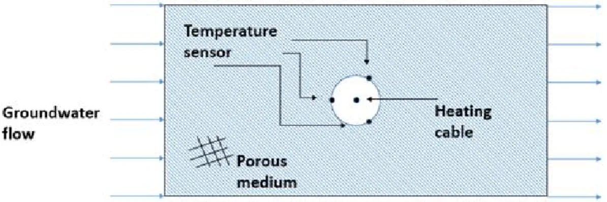
Les tests de réponse thermique actuels, qui sont utilisés afin d’évaluer la conductivité thermique d’un champ géothermique, ne sont pas conçu pour considérer les écoulements d’eau souterrains. Pour mesurer les paramètres de ces écoulements, un nouveau concept a été développé. Des câbles de chauffage sont installés dans un puits qui se trouve en contact direct avec la formation souterraine. Ces câbles sont entourés de trois capteurs de température placés de manière stratégique au périmètre du puits. L’étude de l’évolution de la température pour chaque capteur durant une période chauffage et une période de restitution thermique permet de déterminer la conductivité thermique du sol, en plus la vitesse et de l’orientation de l’écoulement d’eau qu’il contient. Des simulations numériques ont été utilisées pour valider le potentiel de ce concept et établir ses limites.

9

Abstract

Current thermal response tests, used to estimate the subsurface thermal conductivity in the geothermal sector, are not designed to take into account groundwater flows. To measure the flow parameters, a new concept has been developed. Heating cables are installed within a borehole in contact to the formation, with three temperature probes strategically located at the edge of the borehole. Study of the evolution of temperature for each probe during both a heat injection phase and a recovery period allows determining ground thermal conductivity, groundwater flow velocity and orientation. Numerical simulations have been used to validate the proposed concept and establish its limits.

10

2.1 Introduction

The increasing demand for clean energy and the growing concerns over global warming and emissions of CO2 have led to a regain of interest for green energies. Over the last

decades, the use of ground-coupled heat pump (GCHP) systems has developed fast. The number of units installed per year in Canada has grown by a factor close to 1 000% between 2000 and 2010 [15]. GCHP systems transfer heat to the ground (or from the ground) for space heating or cooling in residential and commercial buildings. For a good sizing of borehole heat exchangers (BHEs), engineers need to properly estimate the thermal properties of the ground. Thermal conductivity is an essential parameter in order to characterize the heat transfer between a ground heat exchanger and the surrounding subsurface. Thermal response tests (TRTs) are used for in situ measurement of the subsurface thermal properties. In a typical TRT, the evolution of the temperature of the water circulating in the BHE is measured at the inlet and outlet of the BHE. Then, using Kelvin’s line source theory, which is based on Fourier’s law of conduction, or based on other models to represent heat transfer around the borehole, it is possible to deduce the ground thermal properties [16][17][18][19][20]. Kelvin’s line source model assumes an infinite, homogenous and isotropic ground in which heat transport in the ground is completely driven by conduction [13].

Unfortunately, the assumptions on which this model relies can turn out to be false. One of the most significant limitations is the lack of consideration of convective heat transfer in the ground. Geothermal borefields can be installed in aquifers. If the geological materials is sufficiently permeable or submitted to a strong hydraulic gradient, groundwater will move through the ground pores or fractures, which affects heat transfer around BHEs [21][22][23]. Since the line source model neglects groundwater flows, it has been shown that TRTs in such cases can provide wrong estimates of the subsurface thermal conductivity [19][24][25][26], and most importantly, oversizing of the BHEs. Advection enhances heat transfer between the BHE and the subsurface, which means that shorter BHEs than in the absence of groundwater flow can be installed to satisfy the same load. Analytical [27][28] and numerical [29][30][31][32] models were established to simulate heat transfer around a BHE with groundwater flow. Nevertheless, current TRTs do not

11

provide information on the hydrogeological information required to size the borefield, namely groundwater velocity and direction.

Accounting for groundwater flows is primordial when designing GCHP systems [6]. In recent works, it has been demonstrated that neglecting groundwater flow in design procedure can induce an overdesign of the borefield length that can go up to 68% [8]. Engineers not only need to consider groundwater flowrate, but the direction of the flow is also an important parameter [7]. These parameters have to be known when applying adequate models for the design of geothermal borefield. Determining such parameters requires hydrogeological tests which might be prohibitive in terms of time and cost when designing and installing a GCHP system. Therefore, there is a need to develop a combined hydrogeological and thermal test to acquire the required estimates of ground properties in the design process.

Another possible point of improvement to current TRTs is to obtain a subsurface thermal conductivity profile instead of an average value. Other alternative tests have been proposed to obtain a profile of the ground properties, with the use of optical fibers [33][34][35] or thermostratigraphy [36]. However, these methods are either highly expensive or require the knowledge of additional data such as the local Earth natural heat flow.

In this paper, we address some of the shortcomings mentioned above by developing a configuration of combined hydro-thermal response tests (H/TRT). This H/TRT is inspired by the work of Raymond [37][38], in which a heating cable is placed in a borehole to inject heat in the subsurface during the TRT. Theoretically, with multiple temperature probes positioned in a horizontal plane around the cable, it is possible to observe the strength and direction of groundwater flow. Using heating cable sections to directly generate heat in the borehole requires less power than conventional TRT and less equipment. It is also possible to obtain a vertical profile of the ground thermal conductivity if the test is simultaneously accomplished at various depths. Continuous heating cables can also be used, but require high tension to provide enough heat.

The objective behind this paper is to use numerical simulations to validate the potential of the concept before performing field experiments. The first part of the paper details the concept and the numerical model that was built to simulate its performance in

12

various possible geological cases. Results are then shown in the following sections. From these results, a methodology is proposed to accurately estimate the subsurface thermal conductivity and groundwater flow parameters.

2.2 Description of the concept

Based on the work of Raymond et al. [37], the proposed concept of H/TRT uses a heating cable placed in a borehole to inject heat in the subsurface. This strategy to inject heat in the borehole has already been numerically validated for the measurement of thermal conductivity [38] and yielded promising results based on in situ testing in U-tube ground heat exchangers [39]. In the present paper, however, the heating cable is installed directly in the “empty” borehole (not in the U-tube) that is in contact with the formation. Moreover, groundwater flows have not been considered thus far in that type of tests, hence the need for an adaptation to account for them. In order to do so, it is proposed to use three temperature sensors (instead of one) to measure the evolution of the temperature in the borehole during the heat injection from the source. These probes are distributed uniformly on the edge of the well (i.e., at an interval of 120 degrees). The cable is positioned at the center of the hole. Since the heat plume generated by the source is deformed in the direction of the groundwater flow, each sensor will monitor different temperature evolutions. Therefore, by comparing every sensor measurement, one could potentially estimate the ground thermal conductivity, along with the groundwater flow parameters (i.e., velocity and orientation). The test is performed in a borehole before it is filled with grout. The proposed setup is sketched in Fig. 2.1.

Figure 2.1 - Schematic representation of the proposed H/TRT setup with groundwater flow.

13

The idea behind the H/TRT is similar to that employed by hydrogeologists measuring the hydraulic head at three different wells to determine groundwater flow velocity and direction [11]. The differences are that temperature is the variable measured instead of the hydraulic head, and the test is performed in a single well. In order to constrain the measurement of groundwater flow parameters within a single well, hydrogeologists can also employ a heat-pulse groundwater flow meter, which uses a similar approach to the proposed H/TRT, but cannot provide estimation of the ground thermal conductivity [12]. Lee and Lam proposed a test where they monitored three concurrent standard TRTs in three adjacent boreholes [40]. Other ways of obtaining hydraulic characterization from temperature data have been suggested in the past [41][42]. Simultaneous TRTs and well tests executed in a single borehole greatly reduce both the duration of the test and the equipment needed.

In the present H/TRT, it is proposed to record the probes temperature for a certain period of heating (e.g., three days), followed by a recovery period (no heating) of equivalent duration. The exact position of the sensors and of the heat source might not be precisely known, which can lead to uncertainties on the measured ground properties. It was found that the recovery period can help to reduce these potential errors since the temperature field tends to become more uniform during recovery [43].

2.3 Mathematical and numerical models

Numerical simulations have been performed in order to establish the potential of the H/TRT approach presented in Section 2. Numerical models are fairly easy-to-use and offer the possibility of measuring precisely the individual impacts of various parameters, such as the subsurface thermal conductivity or the groundwater flow rate. Heat transfer in the presence of groundwater flow is a complex process that combines both conduction and advection. The finite element method (FE) has been used to simulate heat transfer and groundwater flow.

14

Table 2.1 Typical groundwater Darcy velocity in various geological materials [44]. Aquifer materials Hydraulic conductivity [m/s] Darcy velocity* _{UD [m/s]} Thermal conductivity kavg [W/mK] Volumetric heat capacity p

c



[10 MJ/m3_K] Gravel 10-4_-10-2 ₁₀-7_-10-5 _{1.8 2.4} Coarse sand 10-3 ₁₀-6 _{1.7-5.0 2.2-2.9} Medium sand 10-4 ₁₀-7 _{1.7-5.0 2.2-2.9} Fine sand 10-6_-10-5 ₁₀-9_-10-8 _{1.7-5.0 2.2-2.9} Silt 10-7 ₁₀-10 _{0.9-2.3 1.6-3.4} Clay 10-10_-10-9 ₁₀-13_-10-12 _{1.2-1.5 2.3}

* Assuming hydraulic gradient of 0.001 m/m

Readers are referred again to Fig. 2.1 to see the numerical domain. It consists of a borehole of radius

r

b embedded in a saturated porous medium. Dry ground is seen as the

matrix of the porous medium and its pores are filled with water (saturated ground). Table 2.1 offers typical values of thermal and hydraulic properties for different geological materials, assuming a hydraulic gradient of 0.001 m/m [44]. While properties for dry ground were consistently modified between each simulation, properties of water used by the model remained fixed and are given in Table 2.2. Preliminary simulations showed that groundwater flow had a negligible impact on TRT for flows with Darcy velocity inferior to 10-8 _{m/s, hence properties of silt and clay were not considered in this study. Materials}

are assumed to be isotropic. Dimensions of the numerical domain were normalized by the borehole radius – its length was 85 times longer than the radius of the borehole while its height was 42.5 times larger. The borehole radius length varied between

r 0.05 m

b



and

b

r 0.1m



_{depending on the simulation case.}

Table 2.2 Properties of water for the numerical model [45].

Properties Value w



[kg/m3_] 999 w



[kg/ms] 1.08 10 3 w

k

[W/mK] 0.598 p,w

c

[J/kgK] 4 184

15

2.3.1 Governing equations

The physical laws governing the problem are the conservation of mass, momentum and energy. In order to limit the computational time, the domain was approximated as two-dimensional. The first two laws are considered in the Navier-Stokes equation, modified to take into account the porous medium. Since the velocity and pressure fields were assumed not to change with time, a steady-state version of the equations was considered:

0 u    _(2.1)







 



2





3  _ _{   } _{    } _         T u u P u u u u          (2.2)

This formulation has the advantage that it is valid both in the ground (porous media with a finite value for the permeability) and in the well itself (where the last term of Eq. (2.2) vanishes). Therefore, the same set of equations can be solved in the entire domain. Far from the borehole, an easy way to approximate the average groundwater flow velocity is to use the Darcy’s velocity:

g r D P u u x         (2.3)

The conservation of energy equation must include both conduction and advection. In a porous medium, it reads as

 

cp _f u



kavg



t     _     _     (2.4) where:

 





 

 

p _f p _s g p f c 1 c T T , c             (2.5)

Note that the index “avg” for k is to indicate the average ground thermal conductivity around the borehole. The values of thermal conductivity and thermal diffusivity depend on the porosity of the ground matrix:





_{ }

avg avg f s avg p f k k k 1 k , c         (2.6)

Other ways to calculate the average conductivity exist. However, it should be noted that what is important for the mathematical modelling of the problem is the thermal conductivity of the porous medium itself, and not the decomposition between the matrix

16

and its pores. Therefore, for simplicity, the arithmetic mean was used to compute the average value of thermal conductivity even though other models are available. Again, the advantage of Eq. (2.4) is that it can be used in the entire domain. In the well, there is only water and no dry ground, meaning that for that part of the domain, conservation of energy is represented by:

 

cp _f u kf  t     _     _     (2.7) In order to limit the number of variables, the problem was solved with dimensionless variables: avg b D b 2 b avg avg b avg avg g 0 f f t ur u r x, y x, y , u ,Pe , Fo , r r 2 k k P , k and P q k                 _(2.8)

Here, presents the heat injection rate of the source during the heating process. The ground effective volumetric heat capacity has to be known for the calculations of Fo and Pe. According to [46], the volumetric heat capacity can be estimated solely based on the identification of the host rock where the borehole is drilled with an uncertainty of±15%. Based on the data from Tables 2.1 and 2.2, ranges employed for each dimensionless scales can be seen in Table 2.3. The velocity vector can be expressed as a product between the Peclet number Pe and a dimensionless vector function:

 

 

u x,y Pe f x,y  (2.9)

Using these scales, Eqs. (2.4) and (2.7) can be reduced to:





Pe f x, y k Fo          (2.10)





Pe f x, y Fo  _{     }  (2.11)

The entire domain is initially at

 

0

. Far from the borehole, the temperature of the boundaries is fixed at the initial value. A pressure gradient is imposed to generate the groundwater flow. While the value of P at the left boundary varies according to the desired groundwater velocity, the dimensionless pressure of the right side remains P 0

0

q



17

for all simulations. This means that groundwater flows in the numerical domain from left to right.

Table 2.3 Simulated range for all variables.

Variable Values tested

Pe 10-3 _{to 10}-1

Fo 0 to 1 000

k 2 to 8

In developing this model, the following assumptions were made:

(i) Local thermal equilibrium is assumed, i.e. water and ground temperatures are the same locally;

(ii) Groundwater flow is assumed to be unidirectional and parallel to the ground surface. Furthermore, groundwater flow is supposed to be present everywhere in the aquifer and to be stationary over the duration of the test;

(iii) The heat transfer is also assumed to be parallel to the ground surface. This assumption is fairly good considering the short periods of time over which tests are performed [47].

(iv) All properties are assumed to be uniform and non-affected by temperature; (v) Dispersivity is not considered explicitly in the model. Although some models account for it [26][44][48], few data is available for quantifying thermal dispersion of typical groundwater flows.

(vi) Natural convection inside the well is neglected. It has been proved that for TRT using heating cable, natural convection can be greatly limited with perforated disks positioned at strategic vertical positions to cut off possible circulating loops [38]. Tests based on the heat-pulse groundwater flow meter usually limits natural convection with the use of packers. Executing the test with continuous heat cable also minimize natural convection if the setup is properly done [49]. Under certain

18

conditions (particularly when the Darcy flow is small), natural convection could have an impact – a 3D model could be helpful to assess this impact.

2.3.2 Numerical model

To solve numerically the above-mentioned differential equations within the domain, a commercial finite element software was used [14]. The mesh generated has unstructured triangular elements that are concentrated around the borehole, where high temperature gradients are expected due to the presence of the heat source. Considering the symmetry of the domain, only half of the domain needs to be simulated. An infinite element zone that was 8.5 time longer than the radius of the borehole was added to the model boundary. It was verified that the domain dimensions had no effect on the simulation results, i.e. that when a larger domain is used, the results stay the same. Time stepping needed to solve the energy equation is automatically chosen by the software during simulation, adjusted with a relative tolerance of ₁₀3_.

To ensure the correctness of the results, mesh convergence was verified. The mesh independence was considered to be reached when doubling the number of elements in the domain yielded a relative discrepancy of less than 1% on the average probes temperature for every time-step in the considered range. The mesh independence study was performed with groundwater flowing far from the borehole at a Peclet number of Pe = 0 and Pe = 0.1. For typical values of

 

eff

10 m / s

6 2 and

r 0.075m

b



, a Peclet number of 0.1 translates

to a Darcy velocity of

u 1.33 10 m / s

D





6 . These correspond to extreme parameter values,

hence the chosen mesh can be applied to every simulation cases if it works for these. The final mesh that was used for simulations contained 7,944 elements and is shown in Fig. 2.2.

19

Figure 2.2 – Mesh of the numerical model used for simulation of the proposed H/TRT setup with groundwater flow.

2.4 Influence of groundwater flow during H/TRT

In order to assess the heat transfer mechanisms during the H/TRT proposed in this paper, numerical simulations were carried out. Simulations were performed to evaluate the impacts of advection on the thermal response of the system. Simulations did not account for variations of



as there is a limited range of possible values for this parameter in typical permeable geological materials. A value of  0.6 was considered for all simulations.

20

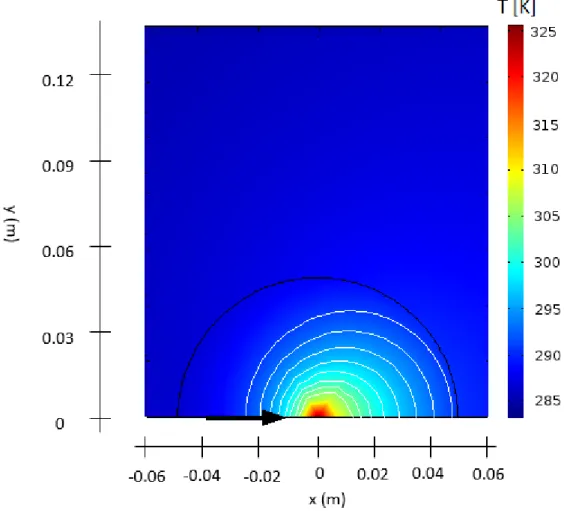
Figure 2.3 - Example of simulated temperature profile in and around the borehole after a day of heating (isotherms with a 2 K increment are shown).

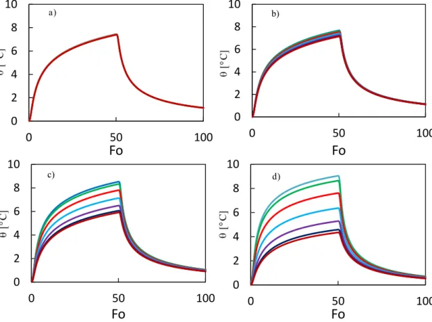
To observe the impact of groundwater flows during the suggested TRT concept, the thermal response created by the heat source was simulated for multiple values of the Peclet number (Pe). Although the influence of advection on the transient evolution of a borehole average temperature has been investigated before, the distribution of temperature produced within the borehole by groundwater flows has received considerably less attention. Fig. 2.3 offers a view of the distribution of temperature in the borehole for a flow of Pe 0.1 , after a day of heating. A ratio of thermal conductivities of k 4 and a power input of 40 W/m for the heat source were used. The center of the borehole, where the cable is positioned, is clearly the warmest area of the domain. The white lines, which represent isothermal lines, are not axisymmetric around the heat source – they are pushed towards the flow orientation, which is represented by the arrow in Fig. 2.3. Therefore, temperature at different positions

21

along the borehole perimeter should read different temperatures. This is confirmed by Fig. 2.4, which presents the thermal response at seven positions along the borehole perimeter at an increment of 30 degrees for four distinct values of Pe. A dimensionless duration of Fo 50 was used for the heating period. The influence of groundwater flow can easily be seen when comparing the curves of Fig. 2.4. Because the heat plume generated by the source stretches in the direction of the flow, sensors that are aligned with the groundwater flow read higher temperatures than the ones that are opposite to the flow, thus creating a difference of temperatures between the sensors. This difference of temperatures widens as Pe increases. In the case of Pe 0.1 , the gap of temperature between sensors is higher than 1°C during most of the heating period, making it possible to notice the influence of subsurface flow. Again, such a Peclet number can easily be reached with a Darcy velocity of

u ~10 m / s

D 6



. On the other hand, the curves for Pe 0.01 are similar to the thermal response of the purely conductive case. As a result, with a heat injection rate of 40 W/m, it appears that the setup cannot properly detect advection at such a low Peclet number value.

Figure 2.4 - Example of temperature evolution measured by sensors for a) Pe = 0.001 b) Pe = 0.01 c) Pe = 0.05 and d) Pe = 0.1. Each color represents a different sensor.

0 2 4 6 8 10 0 50 100

Fo

a) 0 2 4 6 8 10 0 50 100

Fo

b) 0 2 4 6 8 10 0 50 100

Fo

c) 0 2 4 6 8 10 0 50 100

Fo

d)

22

As expected, for all Pe values, during the recovery stage, differences of temperature quickly vanish as temperature in the borehole becomes uniform in a short period of time. A uniform temperature in the borehole can be beneficial because of the evaluation the thermal conductivity becomes less sensitive to the exact position of the cable and sensors within the borehole. Additionally, since the borehole itself is included in the radius of influence of the H/TRT around the heating cable during the injection phase, and since the borehole is filled only by water (which has a low thermal conductivity), a thermal conductivity determined during the heating phase would tend to underestimate the ground thermal conductivity. During the recovery phase, the uniform temperature in the water fixes this issue as there is no heat transfer in the borehole itself as Fo increases.

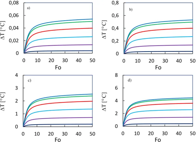
Figure 2.5 - Example of the evolution of the differences of temperature between sensors for a) Pe = 0.001 b) Pe = 0.01 c) Pe = 0.05 and d) Pe = 0.1. Each color represents the difference of

temperature between the probe installed at the warmest position and a different probe. 0 0,02 0,04 0,06 0,08 0 10 20 30 40 50

Fo

a) 0 0,2 0,4 0,6 0,8 0 10 20 30 40 50

Fo

b) 0 1 2 3 4 0 10 20 30 40 50

Fo

c) 0 2 4 6 8 0 10 20 30 40 50

Fo

d)

23

Concerning the differences of temperature between the sensors, it was found that they build up quickly in the early stage of the heating period



Fo 10



. Rapidly, despite of the fact that no steady-state condition is reached, the differences of temperature follow a nearly-constant evolution and progress slowly. In other words, the temperature increases at the same pace for all sensors. This pattern was the same for all Pe as presented in Fig. 2.5. It shows the difference of temperature between the sensor reading the highest temperature and the six other probes.

2.5 Proposed methodology for H/TRT analysis

Section 4 has shown the impact of groundwater flow during the thermal response of the H/TRT setup. The object of the H/TRT is to determine three main parameters: the ground effective thermal conductivity, the groundwater flow velocity and orientation. By evaluating properly the thermal response, it could be possible to isolate the impact of each of these parameters and then to estimate their values. Here, a method to do so will be developed.

2.5.1 Evaluation of the groundwater flow orientation

Since the determination of the flow orientation does not require a particular knowledge of ground properties and is helpful for the estimation of Pe, it is suggested to start the analysis there. A methodology similar to that used in hydrogeology is proposed to find the orientation of the groundwater flow from an H/TRT. In hydrogeology, the path of a subsurface flow is found by locating the equipotential lines. Equipotential lines are the lines where the hydraulic head remains constant. Since the motion of water is strictly driven by the hydraulic gradient, the flow has to be perpendicular to such lines in an isotropic medium. Therefore, if the hydraulic head is known at three different horizontal positions, it is possible to interpolate the direction of equipotential lines and thus to know the orientation of the flow. Although this method is relatively precise, it has the disadvantage that it requires three boreholes to be drilled.

Here, instead of the hydraulic head, it is the temperature that is measured at three distinct positions within a single borehole. This means that the suggested setup cannot

24

directly determine equipotential lines, but it allows users to identify the isothermal lines, hence a similar approach can be used. The direction of the flow was estimated to be the parallel to the gradient of the plane formed by the temperature values measured at the three sensor points. Since advection carries the heat generated by the source in the flow direction, the heat plume described by isothermal lines should be parallel to the motion of groundwater (Fig. 2.3). Simulations were performed to verify this hypothesis and assess the measurement error on the flow direction adopting this method, for different values of Pe. Table 2.4 shows the outcome of this investigation, which was done with k 4 and a

heat rate of 40 W/m. It shows the flow direction determined from the isotherms compared to the actual orientations, for three cases. This study was repeated for different ratios of conductivities, and the results were similar as will be shown later. To correctly represent real thermal sensors, temperatures calculated with the numerical model were rounded to the nearest tenth. In most cases whenPe 0.005 , the setup is not sensitive to groundwater flow and therefore the orientation measurement was impracticable. However, the impact of the groundwater flow on the heat transfer between the borehole and the ground is negligible for these values of Darcy velocity, and therefore, for the sizing of boreholes, this data is actually not that useful. In other words, the knowledge of the flow orientation is not vital at low Pe numbers. When Pe is higher, the error on the measurement was found to be inferior to 15°. The method was more effective for a flow of Pe 0.05 than a flow of Pe 0.1 . This is caused by the fact that the heat plume generated by the source becomes narrower for great velocities. Sensors located outside of the plume are not affected by the heat source which can lead to wrong estimate of the orientation. The temperature measurements were taken at the end of the heating stage in this study.

Table 2.4 Direction calculated after a day of heating for different groundwater velocities. Peclet number

Pe [-] Calculated direction



  _true 70



[°] Calculated direction



 _true 147



[°] Calculated direction



 _true 271



[°]

0.005 60.0 138.2 270.0

0.01 74.5 145.2 263.1

0.05 72.5 143.1 268.4

25

2.5.2 Evaluation of groundwater flow velocity

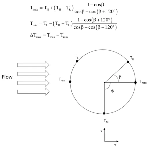
Referring back to Figs. 2.4 and 2.5, it can be seen that the main effect of the groundwater flow velocity is to increase the differences of temperature measured by the sensors on the periphery of the borehole. This increase happens during the early stage of the heating period and the differences of temperature are nearly constant later. Accordingly, the maximal difference of temperature on the borehole perimeter



T

max appears to be

essentially proportional to the flow velocity. As shown in Fig. 2.6,



T

max is defined as the

difference of temperature between two sensors on the borehole perimeter that would be aligned in the direction of the flow, i.e. one upstream and one downstream. In practice, if the flow orientation  is known and a gap of temperatures is sensed between each sensor,

a trigonometric calculation gives a good approximation of



T

max via extrapolation:





_

_







_



_

max H H L

min L H L

max max min

1 cos T T T T cos cos 120 1 cos 120 T T T T cos cos 120 T T T                          (2.12)

26

Equations (2.12) assumes that the temperature field in the borehole can be approximated by a plane. Note that the angle  used in Eq. (2.12) is not necessary equal to

- is the angle between the flow orientation and a reference x-axis and  is the angle

between the flow and the sensor with the highest temperature value, which is not necessarily along the reference axis. To reduce the number of variables,



T

max has been

translated into a dimensionless parameter:

f max max 0 k T T q     (2.13)

Equations (2.12) shows that the extrapolation of



T

max depends on the value of the flow

orientation taken into account by the angle . As a result, the accuracy of the extrapolation

is influenced by the evaluation of . Table 2.5 shows how dependent the determination of

max

T



_{is to the flow orientation. For the sake of illustration, the test was done with} k 4

and Pe = 0.05 at a flow orientation of  30.



T

max was calculated at Fo = 50. Other sets

of parameters were also considered with similar results. The table shows that Eqs. (2.12) provide a satisfying estimate of



T

max even when  is not precisely known. When the error

on the flow orientation evaluation is lower than ±20°, extrapolating



T

max with Eqs. (2.12)

leads to accurate results (errors smaller than 10%).

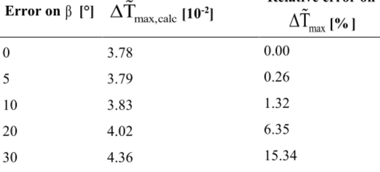
Table 2.5 Error on the extrapolation of the maximal difference of temperature calculated with Eqs.

(2.12) according to the accuracy of the flow orientation measurement ( 2

max,true

T 3.78 10

   ).

Error on  [°] _Tmax,calc[10-2_] Relative error on

max

T



[%] 0 3.78 0.00 5 3.79 0.26 10 3.83 1.32 20 4.02 6.35 30 4.36 15.34

27

Since the value of



T

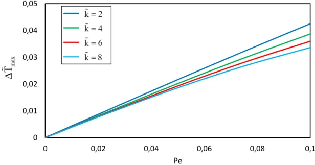
_max evolves with time, it was decided to evaluate it at a given Fourier number. Doing so, the only remaining independent variables are Pe and the ratio of thermal conductivities. Fig. 2.7 shows the evolution of



T

max according to these two

parameters. Data were extracted at a dimensionless time of Fo 10 during the heating stage. This Fourier value was chosen because it was observed that the difference of temperature between sensors changes slowly for Fo 10 . Fig. 2.7 reveals that one can find the subsurface flow Peclet number as long as the difference of temperature is large enough since



T

max is nearly linearly dependent on Pe. k merely changes the slope of the line

function between Pe and



T

max. Its impact is only observable for high values of Pe



i.e. Pe 0.02



, but neglecting the ratio of conductivities can lead to error that are up to 20% when Pe 0.1 and thus must not be completely ignored.

Figure 2.7 - Maximum dimensionless difference of temperatures on the borehole wall versus the flow Peclet number.

0 0,01 0,02 0,03 0,04 0,05 0 0,02 0,04 0,06 0,08 0,1 Pe

28

2.5.3 Evaluation of thermal conductivity

The ground thermal conductivity can be estimated during the recovery period by curve-fitting the evolution of the average borehole wall temperature b

 

Fo calculated by a

model to the one that is observed in the borehole temperature once it becomes uniform. To do that, it is approximated that the average temperature of the borehole wall is equal to the mean value of the three thermal sensors. Calculated temperature evolution can be obtained using a dimensionless ground function G Fo

 

, that is used to determine the temperature increment during heat injection:

 

0

 

b avg q Fo G Fo k    _(2.14)

Once heat injection is stopped, the temporal superposition principle can be used to calculate

 

b Fo  _:

 

0



 







b Heat avg q Fo G Fo G Fo Fo k      _(2.15)

where

Fo

H is the Fourier number when heat injection is stopped.

2.5.3.1 Time needed for the temperature in the borehole to be uniform

Simulations were carried out to provide an estimation of the dimensionless time required to reach temperature uniformity in the borehole

Fo

U once the heat source is turned off. The

temperature uniformity criterion was arbitrarily set at 0.1°C everywhere in the borehole. Uniformity of temperature within the borehole is not necessarily reached when all three sensors have the same reading as the middle of the borehole could be warmer due to presence of the heat source. To circumvent this problem, it is possible to place a fourth sensor near the source to directly find the moment when the temperature is uniform or the results presented here can be used to get an estimate. The simulations showed that there is a logarithmic relation between

Fo

Heat and

Fo

U:









'

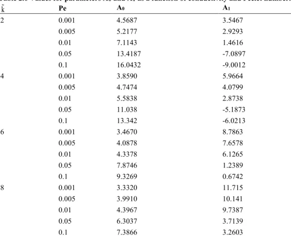
U 0 0 Heat 1

29

where A and B are functions of Pe and k. Table 2.6 provides the values of A0 and A1 for

different sets of Pe and k. The time required for the temperature to become uniform during thermal recovery increases for fast flows, but remains relatively short for grounds with high thermal conductivity. The value of

Fo

U can be estimated either from calculations done

during the heating period or from regional data. In most cases, it is smaller than

Fo

Heat.

Table 2.6 Values for parameters A0 and A1 as a function of conductivity and Peclet number.

k Pe A0 A1 2 0.001 4.5687 3.5467 0.005 5.2177 2.9293 0.01 7.1143 1.4616 0.05 13.4187 -7.0897 0.1 16.0432 -9.0012 4 0.001 3.8590 5.9664 0.005 4.7474 4.0799 0.01 5.5838 2.8738 0.05 11.038 -5.1873 0.1 13.342 -6.0213 6 0.001 3.4670 8.7863 0.005 4.0878 7.6578 0.01 4.3378 6.1265 0.05 7.8746 1.2389 0.1 9.3269 0.6742 8 0.001 3.3320 11.715 0.005 3.9910 10.141 0.01 4.3967 9.7387 0.05 6.3037 3.7139 0.1 7.3866 3.2603

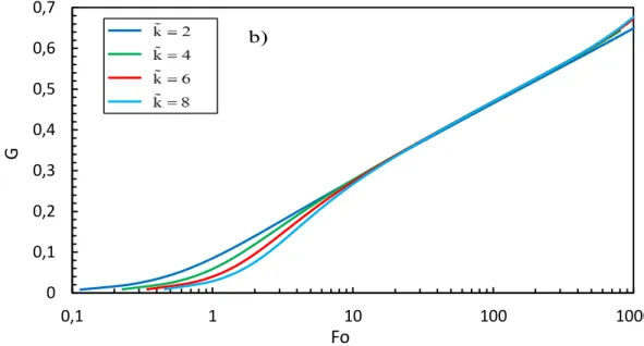
2.5.3.2 Ground function for various Pe and

Advection not only leads to different temperatures read by each sensor, it also alters the temporal development of the mean temperature value of these sensors. A high k value means that the subsurface has a high thermal conductivity compared to the one in the borehole and as a result, heat quickly travels out of the borehole area. Thus the ratio of thermal conductivities also affects the mean temperature value of the borehole perimeter.

30

From Eq. (2.14), this implies that the G-function has to be adapted with Pe and k. This subsection offers a tool to estimate G Fo

 

. Fig. 2.8 presents G Fo

 

for different values of Pe and of k, directly given by the numerical model. For short time-scales, while Pe has no effect on the G-function, G Fo

 

is highly influenced by k. The impact of k is only observable for Fo 10 . Then, for longer time scales, advection comes in and the groundwater flow starts to dominate the heat transfer process over radial conduction. The critical Fourier

Fo

c separating these two states highly depends on Pe. While

Fo 10

c



for

flows of Pe 0.1 , this value increases up to

Fo 250

c



when Pe 0.025 . These critical

values can be used to determine the limit of the pure conductive stage if one wants to use the line-source theory to deduce the effective thermal conductivity during the heating period. In spite of the presence of groundwater flows, typical TRT durations are not long enough for the system to reach a steady-state, unless the test is executed in an unusually high permeable aquifer



Pe 0.1



. With the dimensionless time range used for this analysis, effects of convection on the G-function become apparent whenPe 0.02 . Not accounting for advection during TRT analysis leads to erroneous estimation of thermal conductivity when the flow Darcy velocity is higher than this value.

0 0,1 0,2 0,3 0,4 0,5 0,6 0,7 0,1 1 10 100 1000 G Fo Pe = 0 Pe = 0.01 Pe = 0.025 Pe = 0.05 Pe = 0.075 Pe = 0.1 a)

31

Figure 2.8 - Ground function for the TRT a) as a function of the Peclet number k=5 , and b) as a

function of the ratio of thermal conductivities (Pe=0.01).

2.5.4 Schematic step-by-step analysis procedure

Figure 2.9 presents a summary of the suggested analysis method in a step-by-step procedure. After the preliminary steps of choosing test parameters, the H/TRT can be executed and then analysed. As previously explained, it is relatively easy to quickly obtain a good estimate for the groundwater flow orientation  from the H/TRT data. Once this evaluation is done, it is possible to extrapolate the dimensionless maximum difference of temperature



T

max on the borehole perimeter using trigonometry. This dimensionless

parameter is linked to the flow velocity number and thus could be used to obtain the Peclet number. However, the relation between



T

max and Pe is affected by the ratio of thermal

conductivities k, which is still unknown. Therefore, an iterative procedure is required and a guess has to be made on the ground thermal conductivity

k

avg. This guess on

k

avg allows

users to convert time values into Fourier numbers Fo and to measure a temporary value for Pe. Following that, curve-fitting on G Fo

 

is needed to get a new value for the ground thermal conductivity. It is preferable to do this curve-fitting when the temperature in the borehole is uniform during thermal recovery since it decreases the impact of an erroneous

0 0,1 0,2 0,3 0,4 0,5 0,6 0,7 0,1 1 10 100 1000 G Fo b)

32

position for the heat source or the sensors due to the absence of heat transfer within the borehole. To find when the temperature in the borehole is uniform, a fourth sensor can be placed within the borehole or Table 2.6 along with Eq. (2.16) can be used. If the curve for the average borehole wall temperature observed in the field fits with the one calculated with G Fo

 

, then the iterative process is complete and the values for Pe and k are final. If not, another iteration is required, going back to the calculation of Pe.

The procedure was numerically tested for numerous situations. To mimic a resolution of 0.1 °C for the temperature sensors, numerical data were rounded to the nearest tenth. Fig. 2.10 shows the results of 25 H/TRT tests with different orders of magnitude for k and Pe. The values for k, Pe, ,

q

'₀,

r

band

t

Heat were randomly selected, but had to fit

within a realistic range (Table 2.3). No more than three iterations were required for each test.

Thermal conductivity values determined by this procedure were all within a range of 10% of the input value in the numerical model as shown in Fig. 2.10a. The methodology has a tendency to underestimate the ground thermal conductivity because of the presence of the borehole which is only filled with water – the fluid thermal conductivity is lower than the ground thermal conductivity, hence the slight underestimation. The use of a cylinder-source model could circumvent the problem. Measurements for the Darcy velocity were accurate when

u

D

10 m / s

7





_{as the measurement error was under} 10% for all situations involving such a flow (see Fig. 2.10b). Below that value of

u

D, measurements

yielded less precise results. The H/TRT might be unable to reveal the groundwater flow when it is too weak. Fortunately, for geothermal applications, it is not needed to know the groundwater flowrate with great accuracy in that range of Darcy velocity. Simply knowing that the flow is weak is good enough for sizing vertical heat exchangers when the velocity is small. Evaluations of the flow orientation (Fig. 2.10c) were relatively accurate when

7 D

u

_

10 m / s



. For slower groundwater flow, the direction estimation methodology is less effective. Obviously, the angle cannot be estimated when the setup cannot sense groundwater flow.

33

34 1 2 3 4 5 1 2 3 4 5 M ea su red kav g [W/ mK] Input k_avg[W/mK]

a)

1,00E-08 1,00E-07 1,00E-06

1,00E-08 1,00E-07 1,00E-06

M ea su red uD [m /s] Input u_D[m/s] b)

35

Figure 2.10 - Comparison between estimates of the parameters obtained from the H/TRT and their actual values for a series of random cases: a) subsurface thermal conductivity b) Darcy velocity

c) flow orientation, and d) required borefield length. (Both values are equal when markers fall on the black dashed line. Red dashed lines correspond to an error of ±10%).

-30 0 30

1,00E-08 1,00E-07 1,00E-06

Err or on [ °] Input u_D[m/s]

c)

1000 1500 2000 2500 3000 1000 1500 2000 2500 3000 M ea su red r eq u ir ed b or ef ield len gt h [m ]

Input required borefield length [m]