Detection of near-field, low permittivity layers
with Ground Penetrating Radar: analytical
estimation of the reflection coefficient
A. Van der Wielen
Belgian Road Research Centre
Boulevard de la Woluwe 42, 1200 Brussels, Belgium [email protected]
L. Courard, F. Nguyen
University of LiegeChemin des Chevreuils, 1, 4000 Liège, Belgium [email protected], [email protected]
Abstract— The reflection coefficient of GPR waves
encountering embedded thin layers is commonly estimated using a plane wave, far field approximation. But when the thin layer is situated in the near field of the antenna, the spherical nature of the waves and the possible propagation of a lateral wave into the layer may have a strong influence on the measured reflected amplitude. In this work, we studied through 2D FDTD simulations the behavior of a radar wave interacting with thin layers of different thicknesses. The snapshots and radargrams showed a large influence of the layer thickness on the wave propagation. For the very thin layers, the evanescent wave plays a major role and the plane wave approximation gives a good estimation of the reflection coefficient. For thicker layers, the specific inclination of each multiple reflection has to be taken into account, as well as the lateral wave propagation. On the basis of these observations, we determined which analytical method should be used for the analytical prediction of the reflection coefficient, as a function of the layer thickness.
Index Terms—GPR, thin layers, lateral wave, spherical
reflection, plane wave approximation, evanescent wave.
I.INTRODUCTION
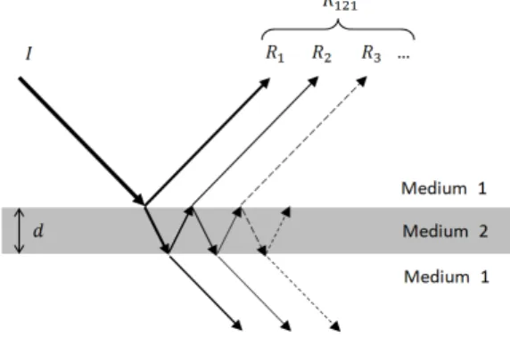
Thin layers are relatively common in civil engineering. For example, the waterproofing layer of a bridge deck presents a large extent for a very low thickness (< 1 cm). The reflection of GPR waves on these layers is complex, due to the multiple reflections on the two interfaces limiting the layers (Fig.1). The determination of the layer parameters requires then a detailed analysis of the reflected wavelet.
Fig. 1. Multiple reflections in a thin layer
Full waveform inversion methods can give good estimation of thin layers parameters [1-3], but they also require an antenna calibration, as well as a large computing cost. The faster alternatives to these methods exploit the reflection coefficient of the layer to determine its properties [4-6]. The reflection coefficient, R, is the proportion of the incident wave reflected by the layer.
Analytical expressions for the reflection coefficient are well known when the layer is sufficiently far from the antennas [7]. But when civil engineering structures are tested, the antenna is seldom in the far field, which will generate the appearance of other phenomena, such as the lateral wave. In this paper, we analyze numerically and analytically the reflection of a GPR wave on a thin air layer embedded into concrete, as a function of the layer thickness. We propose a method allowing the reflection coefficient to be estimated for every layer thickness.
II.ANALYTICAL DESCRIPTION OF THE REFLECTION PHENOMENA
In this section, the equations of two different methods for the estimation of the reflection coefficient of simple interfaces are detailed. Two different methods for the estimation of the global reflection of a thin layer are presented as well.
A.Reflection coefficient of plane waves
The reflection and transmission coefficients R and T for a plane wave reflected by the interface between two materials of relative dielectric permittivities ε’r1 and ε’r2, with the incidentangle θ1 can be calculated by the Fresnel formulas (1)-(2). These equations are valid in the transverse electric mode (TE) and for low-loss materials [7, 8]:
The amplitude of the reflection coefficient is equal to 1 when the incident angle is larger than the critical angle θcr:
This situation only occurs when the deeper material has a lower permittivity than the surface one. The term under the square root in (1) is then negative: the reflection coefficient becomes a complex number. The reflected wave has the same amplitude as the incident one (Fig. 3.) but with a different phase.
With this postcritical incidence, no power is transmitted to the second medium but a field is generated along the interface: the evanescent field. This evanescent wave will be observable in the propagation snapshots of Fig. 5.
The transmission coefficient calculated with equations (1) and (2) can be applied without modification to estimate the evanescent wave [9], whose amplitude decreases exponentially with the distance from the interface [10, 11]. It propagates into the second medium with an imaginary angle of energy transfer which can be calculated using Snell’s equation:
Despite its fast amplitude decay and its lack of power, the evanescent wave cannot be neglected in all cases. Indeed, if a second interface is present close to the first one, in the zone where the evanescent wave amplitude is not negligible, the wave can be reflected by this second interface and become propagative again [12]. This situation will occur when very thin layers are inspected with GPR.
B.Reflection of spherical waves
When the incident wave is spherical and not plane, the Fresnel reflection coefficient can be used as an approximation, but it is not exact anymore [13, 14]. The actual reflection coefficient, R12, spherical presents a deviation that can be considerable in the neighborhood of the source, if the dielectric parameters of the materials are very similar or in the vicinity of the critical angle [13]. The apparent reflection coefficient will then be frequency dependent.
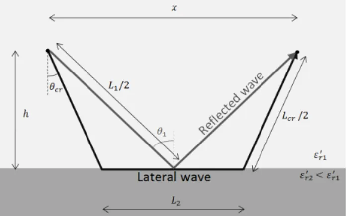
In addition to this modified reflection coefficient, a lateral wave will also appear. This wave meets the thin layer with an incident angle equal to the critical angle and travels at the interface between the surface medium and the thin layer (Fig. 2). The amplitude of the lateral wave at the receiver can be estimated through a pseudo-reflection coefficient Rlateral [13]. The global reflection coefficient for a spherical wave Rspherical is then the sum of those two events:
Fig. 2. Representation of the ray propagation of a spherical wave. If n is the refractive index:
the reflection coefficient for the simple reflection of the spherical wave at the interface between the materials 1 and 2 is given by (7):
With
For incident angles larger than the critical angle, the reflection coefficient of the lateral wave is equal to [13, 14]:
In (10), Lcr, L2 and x are parameters linked to the geometry of the reflection (Fig. 2). k1 and k2 are the propagation constants of the materials and depend on the wave pulsation ω as well as on the speed v and attenuation coefficient α in the materials:
In (7) and (10), µ(β) and F(η) are functions enclosing complex integrals which do not have analytical solutions. Nevertheless, they can be approached for specific values by asymptotic expansions [14] or, more efficiently, be
evaluated numerically for all values. They depend on β and
η, two functions related to the dielectric properties of the
materials and to the geometry of the reflection [13]. Equations (5)-(11) are based on exact solutions approximated by high-frequency asymptotic methods [13]. Those approximations are totally valid when the source-interface distance is sufficiently important, when the propagation constant k1 is high and for interfaces with a low velocity contrast. These conditions are not totally respected in the configurations and distances used in this work; the equations can thus only be considered as approximations.
In Fig. 3, the reflection coefficients calculated by the spherical equations (5)-(11) and by Fresnel equation (1) are compared to reflection coefficients obtained through 3D FDTD modelling (with the program GprMax [15]), in the case of a concrete (ε’r1=7.7) - air interface situated at a distance of 10 cm from the investigation line. The numerical reflection coefficient is obtained by dividing the measured amplitude by the amplitude reflected by a perfect reflector [16]. The tests are performed for an incident frequency of 2.3 GHz.
The estimations computed with the spherical equations are much closer to the numerically estimated reflection coefficient than the curves obtained with Fresnel equations. In particular, the oscillations due to the interaction with the lateral wave for large angles clearly appear in the modelling results. The difference between Fresnel and spherical predictions is the most important at the critical angle. At this point, the reflection coefficient predicted by Fresnel equations overestimates the numerical reflection coefficient by more than 50%, while the difference with the spherical equations is smaller than 2%.
C.Reflection on thin layers
The global reflection of a thin layer corresponds to the sum of all the multiple reflections (Fig. 1). If the incident wave can be considered as plane, i.e. the difference of inclination of each multiple can be neglected, the geometric series formula allows to transform the infinite series into the simple, well-known [4, 7] equation:
0 10 20 30 40 50 60 70 0 0.2 0.4 0.6 0.8 1 R e fl e c ti o n c o e ff ic ie n t a m p lit u d e Incident angle (°) Spherical equations 3D FDTD simulations Fresnel equations
Fig. 3. Comparison of the amplitude of the reflection coefficients estimated with Fresnel and spherical equations to the coefficients measured
through 3D modelling.
In (12), the reflection coefficient for a simple interface
R12 can be calculated using (1).
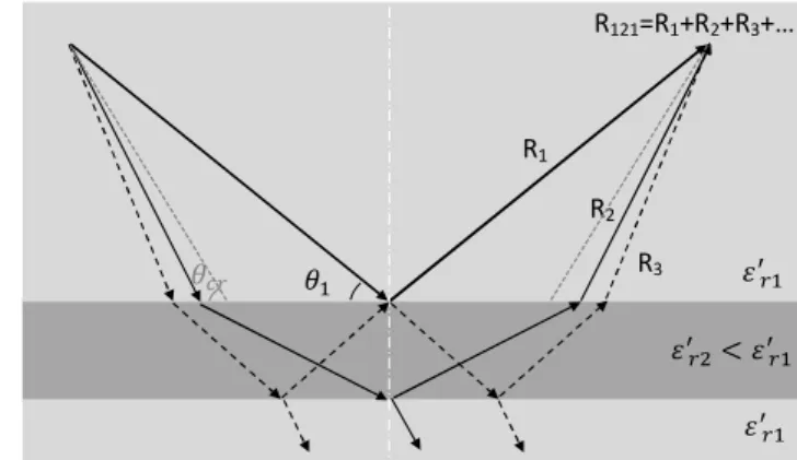
If this plane wave approximation is not valid, it is possible to evaluate numerically the n first terms of the series, with the actual incident angle geometrically determined for each one of them. For each path, the different reflections are calculated using Fresnel equations (1)-(2) [16]. We will refer to this method as the first terms estimation:
When the wave has a vertical incidence, both methods give the same results. But when the incident angle is large, the paths of the rays get more and more different, especially if the layer has a lower permittivity than the matrix. Indeed, the incident angles remain inferior to the critical angle for the first terms estimation (Fig. 4), while they remain equal to the initial angle θ0 with the plane wave approximation.
In this case, the multiples calculated by the two methods are very different, and correspond in fact to two different sets of waves travelling in reality. The multiple reflections
R2 - Rn calculated by the plane wave approximation (12) correspond to the evanescent wave and its different reflections into the layer. Indeed, these reflections are calculated from the first reflection coefficient, whose amplitude is equal to 1 for large angles. The transmitted wave is thus evanescent, propagating with an imaginary angle and becoming propagative again by reflecting on the second interface.
On the other hand, the exact estimation of the first terms (13) does not take into account this evanescent wave, because the multiple reflections are calculated for incident waves under the critical angles (Fig. 4).
R1 R2 R3 R121=R1+R2+R3+…
Fig. 4. Thin layer reflection of a spherical wave for incident angle superior to the critical angle, for the first terms estimation.
III.OBSERVATION OF THE WAVE PROPAGATION To understand the propagation of GPR waves when encountering embedded layers, we performed numerical simulations of the propagation of a GPR pulse into concrete encountering air layers of different thicknesses. In Fig. 5, the snapshots for the layers of 1 cm and 10 cm are displayed.
The wave propagation is totally different for thin and thick layers. No visible wave front propagates into the 1 cm layer, which means that the multiple reflections and the lateral wave are highly attenuated. Simultaneously, the amplitude of the evanescent wave has not decreased to zero yet when encountering the second interface: this wave will reflect and become propagative again. A similar behavior is observed for the thicknesses smaller than 0.3 λ.
On the other hand, when the thickness is larger than 0.5 λ, the evanescent wave is equal to zero when reaching the second interface. However, the wave front of the multiple reflections and of the lateral wave can be observed in the layer. For the layers with intermediate thicknesses (0.3 λ - 0.5 λ), the observed behavior is intermediate [16].
(a) 1 cm D E S (b) 10 cm D E S L+R1+R2+…
Fig. 5. 2D snapshots of the 2.3 GHz wave propagation from concrete (ε’r=7.7) to air layers of (a) 1 and (b) 10 cm. D, S, L, Ri and E are the direct
wave, the source, the lateral wave, the secondary reflections and the evanescent wave, respectively.
It is thus expected that the reflection coefficient will have to be described by different equations, depending on the layer thickness.
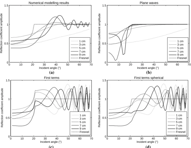
IV.COMPARISON OF THE NUMERICAL REFLECTION COEFFICIENT TO THE ANALYTICAL PREDICTIONS In Fig. 6. (a), we plotted the reflection coefficient amplitude measured by 3D FDTD simulations as a function of the incidence angle and for different layer thicknesses.
The behavior observed in the snapshots (Fig. 5.) is confirmed: for the thin layers, the evolution of the reflection coefficient is smooth, which means that no constructive and destructive interferences can be observed between the wave front in the layer and the first reflection.
In Fig. 6 (b) the same curves are calculated with the method of the plane wave approximation (12). It gives a good estimation of the numerical reflection coefficient for the thinner layers (1 cm and 3 cm).
In the curves calculated with the first term estimation (13), represented in Fig. 6 (c), the oscillations corresponding to the interaction between the two wave fronts appear, but the results are far from the predictions, even for the thickest layers. Indeed, a sharp slope discontinuity is observed at the critical angle, and the amplitude of the oscillations after the critical angle does not decrease as expected.
The discontinuity at the critical angle is due to the use of Fresnel equations, that does not describe well the reflection of spherical waves nor the propagation of the lateral wave. To take these phenomena into account, we calculated the first reflection R1 in (13) by using the spherical reflection equations (7)-(11) instead of Fresnel equations (Fig. 6 (d)).
With this ‘First terms spherical’ method, the discontinuity at the critical angle is strongly attenuated, giving a fair estimation of the numerical reflection coefficient at the critical angle, and even for angles up to about 35°. For larger angles, the method overestimates the oscillations of the curves. An attenuation function should be introduced in the equations in order to be able to reach a good estimation of the reflection coefficient for all incident angles and layer thicknesses.
V.CHOICE OF THE BEST ANALYTICAL MODEL AS A FUNCTION OF THE LAYER THICKNESS
Under the observations of the previous sections, we can conclude that the best model for the estimation of the reflection coefficient of a thin layer depends on the layer thickness [16]:
- for very thin layers (under 0.3 λ), or for layers presenting a higher permittivity than the matrix, the plane waves approximation (12) may be used; for thick layers (above 0.5 λ), the method giving the best results is the first terms methods (13), with calculation of the first reflection by the spherical equations (7)-(12). This method is valid only for incident angles up to 120% the critical angle. To be able to characterize larger angles, a specific attenuation function should be introduced;
0 10 20 30 40 50 60 70 0 0.5 1 1.5 R e fl e c ti o n c o e ff ic ie n t a m p lit u d e Incident angle (°)
Numerical modelling results
1 cm 3 cm 5 cm 7 cm 9 cm Fresnel 0 10 20 30 40 50 60 70 0 0.5 1 1.5 R e fl e c ti o n c o e ff ic ie n t a m p lit u d e Plane waves Incident angle (°) 1 cm 3 cm 5 cm 7 cm 9 cm Fresnel (a) (b) 0 10 20 30 40 50 60 70 0 0.5 1 1.5 R e fl e c ti o n c o e ff ic ie n t a m p lit u d e Incident angle (°) First terms 1 cm 3 cm 5 cm 7 cm 9 cm Fresnel 0 10 20 30 40 50 60 70 0 0.5 1 1.5 R e fl e c ti o n c o e ff ic ie n t a m p lit u d e Incident angle (°)
First terms spherical
1 cm 3 cm 5 cm 7 cm 9 cm Fresnel (c) (d)
Fig. 6. Reflection coefficient amplitude versus incident angle curves of air thin layers of different thicknesses into concrete : (a) estimated through 3D FDTD modelling, (b) calculated with the plane wave approximation method, (c) calculated with the first terms estimation method and (d) calculated with
the first terms method modified with the spherical equations. - for the intermediate layers (0.3 λ - 0.5 λ), we
suggest to calculate the reflection coefficient on the basis of a linear interpolation between the two previous methods.
VI.CONCLUSION AND PERSPECTIVES
The behavior of radar waves, when encountering thin layers in the near field with a postcritical incidence, is dependent on the layer thickness. For very thin layers, the reflection of the evanescent wave on the second interface is predominant, while the propagation of the multiple reflections and of the lateral wave into the layer is almost inexistent. For large layers, the influence of the evanescent wave can be neglected; the propagation of the multiple reflections and of the lateral wave into the layer highly influences the global reflection coefficient, even if those waves are submitted to an attenuation influenced by the layer thickness.
Therefore, the best equations for the prediction of the reflection coefficient of an embedded layer will depend on the layer thickness. The plane wave approximation is valid for thin layers while, for thicker layers, better results are obtained by using the first terms method with introduction
of the spherical equation. In this second case, the results for the large incident angles could be improved by the introduction of an attenuation function for the oscillations of the reflection coefficient amplitude.
The analytical evaluation of the reflection coefficient may be exploited as the forward solution of an inversion procedure, or as a fast pre-evaluation of the layers parameters, in order to reduce the parameters space before the use of a more sophisticated method.
However, when the tests are performed with surface antennas, additional surface phenomena will appear and influence the measured amplitude. For example, a surface lateral wave, travelling along the surface after reflecting on the thin layer with the critical angle, will be measured simultaneously to the lateral wave travelling into the layer [16]. To efficiently exploit the analytical results presented in this paper for field data inversion, it will be necessary to develop a mathematical expression of this surface-lateral wave similar to (10). Other parameters that should be accounted for in order to obtain a comprehensive forward model for the radar measured amplitude are the variations of the antenna-medium coupling and the antenna radiation pattern.
ACKNOWLEDGMENT
This research was founded by the FNRS, under the research fellow grant FC 84664 and finalized thanks to the financial support of the University of Liege.
REFERENCES
[1] C. Patriarca, S. Lambot, M. Mahmoudzadeh, J. Minet, and E. Slob, "Reconstruction of sub-wavelength fractures and physical properties of masonry media using full-waveform inversion of proximal penetrating radar," Journal of Applied Geophysics, vol. 74, pp. 26-37, 2011.
[2] S. Lambot, A. P. Tran, and F. André, "Near-field modeling of radar antennas for wave propagation in layered media: when models represent reality," in 14th International Conference on Ground Penetrating Radar (GPR), 2012, pp. 42-46.
[3] S. Busch, J. van der Kruk, J. Bikowski, and H. Vereecken, "Quantitative conductivity and permittivity estimation using full-waveform inversion of on-ground GPR data," Geophysics, vol. 77, pp. H79-H91, 2012. [4] J. Deparis and S. Garambois, "On the use of dispersive
APVO GPR curves for thin-bed properties estimation: Theory and application to fracture characterization," Geophysics, vol. 74, pp. J1-J12, 2009.
[5] I. L. Al-Qadi and S. Lahouar, "Measuring layer thicknesses with GPR - Theory to practice," Construction and Building materials, vol. 19, pp. 763-772, 2005.
[6] C. Grégoire and F. Hollender, "Discontinuity characterization by the inversion of the spectral
content of ground-penetrating radar (GPR) reflections - Application of the Jonscher model," Geophysics, vol. 69, pp. 1414-1424, 2004.
[7] A. P. Annan, "Ground-Penetrating Radar," in Near-Surface Geophysics Part 1: Concepts and Fundamentals, D. K. Butler, Ed., ed: Society of Exploration Geophysicists, 2005, pp. 357 - 438. [8] A. Annan, "Ground penetrating radar workshop notes,"
Sensors and Software Inc., Mississauga, Ontario, 2001. [9] J. C. White, "Development and application of the phase-screen seismic modelling code," Durham University, 2009.
[10] R. Shevgaonkar, Electromagnetic waves: Tata McGraw-Hill Education, 2005.
[11] C. Chapman, "Basic wave propagation," in Fundamentals of seismic wave propagation, ed: Cambridge University Press, 2004.
[12] F. de Fornel, Evanescent waves: from Newtonian optics to atomic optics vol. 73: Springer, 2001.
[13] V. Červený and F. Hron, "Reflection coefficients for spherical waves," Studia Geophysica et Geodaetica, vol. 5, pp. 122-132, 1961.
[14] L. M. Brekhovskikh and R. T. Beyer, Waves in layered media vol. 4: Academic press New York, 1960.
[15] A. Giannopoulos, "Modelling ground penetrating radar by GprMax," Construction and Building materials, vol. 19, pp. 755-762, 2005.
[16] A. Van der Wielen, "Characterization of thin layers into concrete with Ground Penetrating Radar," Ph.D Thesis, University of Liège, 2014.