Functional data analysis applied to the multi-spectral correlated– k distribution model

HAL Id: hal-01648752

https://hal.archives-ouvertes.fr/hal-01648752

Submitted on 22 Mar 2018

HAL is a multi-disciplinary open access

archive for the deposit and dissemination of

sci-entific research documents, whether they are

pub-lished or not. The documents may come from

teaching and research institutions in France or

abroad, or from public or private research centers.

L’archive ouverte pluridisciplinaire HAL, est

destinée au dépôt et à la diffusion de documents

scientifiques de niveau recherche, publiés ou non,

émanant des établissements d’enseignement et de

recherche français ou étrangers, des laboratoires

publics ou privés.

Functional data analysis applied to the multi-spectral

correlated– k distribution model

Longfeng Hou, Mathieu Galtier, Vincent Eymet, Frédéric André, Mouna

El-Hafi

To cite this version:

Longfeng Hou, Mathieu Galtier, Vincent Eymet, Frédéric André, Mouna El-Hafi. Functional data

analysis applied to the multi-spectral correlated– k distribution model. International Journal of

Ther-mal Sciences, Elsevier, 2018, 124, pp.508-521. �10.1016/j.ijtherTher-malsci.2017.10.005�. �hal-01648752�

Functional data analysis applied to the multi-spectral correlated–k

distribution model

Longfeng Hou

_{, Mathieu Galtier}

_{, Vincent Eymet}

_{, Frederic André}

_{, Mouna El Hafi}

a_{University of Shanghai for Science and Technology, School of Energy and Power Engineering, Shanghai, 200093, PR China} b_{Univ Lyon, CNRS, INSA-Lyon, Université Claude Bernard Lyon 1, CETHIL UMR5008, F-69621, Villeurbanne, France} c_{Méso-Star SAS, 8 rue des pêchers, 31410 Longages, France}

d_{Université Fédérale de Toulouse Midi-Pyrénées, Mines Albi, UMR CNRS 5302, Centre RAPSODEE, Campus Jarlard, F-81013, Albi CT Cedex, France}

A B S T R A C T

The Ck (Correlated-k) approach is among the most used method for the approximate modelling of the radiative properties of gases both in uniform and uniform media. One of its main defects is that the treatment of non-uniform gas paths is founded on the assumption of correlation - in fact co-monotonicity - of gas absorption coefficients in distinct states which is not rigorously verified for actual spectra. This correlation assumption fails as soon as large temperature gradients are encountered along the radiative path lengths. In order to circumvent this problem, a method based on functional data analysis (FDA) referred to as the MSCk model in this work -was proposed in Refs. [1,2]. The principle of the method is to group together wavenumbers with respect to the spectral scaling functions - defined as the ratio between spectral absorption coefficients in distinct states - so that the correlation/co-monotonicity assumption can be considered as exact over the corresponding intervals of wavenumbers. Very few details were provided up to now about the application of FDA within the frame of the MSCk model. Indeed, most of our previous works were dedicated to the derivation of the methods itself. Accordingly, in the present paper, we mostly focus our attention on the mathematical definition of clusters of scaling function, quantities which are used to build spectral intervals over which gas spectra in distinct states are assumed to be scaled. The comparison of different clustering methods together with the criterion to select an appropriate number of clusters are described and discussed and the application of this approach for several test cases, including 3D geometries, are presented.

1. Introduction

Radiative heat transfer in gaseous media plays a key role in a wide range of industrial applications: high temperature combustion cham-bers [3], gas turbine combustors [4], long-range IR sensing[5], fire safety[6], etc.

In all these applications, evaluating the radiative heat transfer in-side the gaseous medium requires modelling its radiative properties over any possible gas path. Among the models available in the litera-ture, the Ck approach is one of the most popular. Its extension in the narrow band (NBCk), full spectrum (FSCk) and the statistical narrow band version (SNBCk) has been discussed by Chu[7]and Consalvi[8]. Chu [7] found that the SNBCk is sufficiently accurate to generate benchmark results for multi-dimensional radiation problems. Consalvi [8]compared several usual radiation models and concluded that NBCk model provides accurate results in the case of axisymmetric pool fires.

However, the main theoretical defect of the Ck model for applica-tions in non-uniform media is that band intervals are treated as a whole, without any verification of the correlation assumption. This leads to the breakdown of the assumption of rank correlation of gas spectra in distinct states when large temperature gradients exist in the medium studied [9]. In order to circumvent this problem, we introduced a method based on functional data analysis (FDA)[10]and called the MSCk model[1,2]. The main ideas behind the MSCk approach are not new, as they share similar concepts as used in mapping methods such as described in West and Crisp[11]or in the multiscale method of Zhang [12]. The objective of this method is in fact to group together wave-numbers according to the spectral scaling functions[1]defined as the ratio between spectra in different thermophysical states. Over these intervals, the correlation assumption can be considered as exact. It has already been shown that the MSCk model with 25 clusters, defined over a narrow band (25 cm−1_{), is more accurate than the medium resolution}

∗_{Corresponding author. University of Shanghai for Science and Technology, School of Energy and Power Engineering, Shanghai, 200093, PR China.} 1E-mail address:_{www.meso-star.com}longfenghou@126.com_. (L. Hou).

(1 cm−1_{) Ck model when compared with LBL benchmark calculations}

at nearly the same computational cost[2]. Meanwhile, the MSCk model has almost the same accuracy as the CKFG (Correlated-k Fictitious Gas) [13]technique in infrared signature cases, but at lower computational costs[14]. Another advantage of the MSCk model, compared to CKFG, is that MSCk can be applied in the case of reflecting walls, which is not compatible with the CKFG model which requires a formulation in terms of transmissivities[2].

The concept of clusters is one of the most important in the building of MSCk model coefficients. In this paper, we mostly focus our attention on the basic mathematical definition of clusters of scaling functions and on the comparison of different clustering methods. The definition of clusters of scaling functions is given in Section2. Comparisons between different clustering methods are discussed in detail in Section3and the arbitrary choice of the number of clusters is addressed in Section 4. Application of the proposed model for current radiative heat transfer calculations is provided in Section5.

2. Clustering scaling functions 2.1. Correlation assumption

In the Ck model, the assumption of co-monotonicity - viz. the pservation of the ranks between spectra in distinct states, originally re-ferred to as rank correlation in Ref. [15]in which this idea was first introduced - is used to extend the k-distribution method from uniform to non-uniform gas paths. The aim of this subsection is to discuss the physical reasons that explain why the correlation assumption is likely to fail in media with high temperature gradients.

The correlation/co-monotonicity assumption can be formulated as follows: for any wavenumberη inside a narrowband ∆η, the absorption coefficientκ ϕη( )at thermophysical conditionϕ can be represented as a function H (strictly monotonic, and more precisely increasing) of κ ϕη( ref), as:

=

κ ϕη( ) H κ ϕ[ (η ref)] (1)

whereκ ϕη( ref)is the absorption coefficient at the same wavenumber in some prescribed reference thermophysical condition ϕref_{. As H is}

strictly increasing by assumption, κ ϕη( ) andκ ϕη( ref) share the same

monotonicity: this means that for any couple of wavenumbersη₁andη₂, if we haveκ ϕη1( ref)>κ ϕη2( ref)in the reference state, then we can draw the conclusion thatκ ϕη₁( )>κ ϕη₂( )in state ϕ at the same spectral lo-cation.

This assumption is accurate as soon as temperature gradients are small along non-uniform paths. This explains why the Ck method has encountered a great success to treat situations which involve small temperature gradients, such as encountered in atmospheric applications [16] [17]or radiative heat transfer in combustion chambers. However, for non-uniform media with large temperature gradients (such as en-countered in remote sensing problems), the correlation assumption between gas absorption coefficients at different temperatures poorly represents the true behavior of gas spectra in distinct thermophysical states. This is mainly due to the appearance of so-called “hot lines”[13] that breaks the one-to-one correspondence between gas spectra as-sumed in Eq.(1).

A solution to this problem consists in building groups of wave-number in such a way that the scaling function, defined as the ratio between the absorption coefficients in state ϕ and in the reference thermophysical condition ϕref_{, is uniform inside each of these groups.}

Built this way, gas spectra are scaled (linearly correlated, on can find more details in Page 321 of Ref.[7]) over the groups, which means that the assumption of co-monotonicity becomes, if not rigorous in practice, at least more relevant over the groups than over the whole band. This is the principle of many methods to improve gas radiation models in non-uniform media such as the multi-scale model by Modest and Zhang or

the multi-spectral technique described in the present paper. Both of these methods are however funded on the same concept of mapping introduced in 1992 by West and Crisp within the frame of radiative heat transfer in non-uniform atmospheres[11].

Fig. 1(inspired fromFig. 4of Ref.[2]) depicts the results obtained by application of the clustering method to a narrow band [1487.5 cm−1_{, 1512.5 cm}−1_{] of H}

2O. Each of the curves corresponds to

the variations of absorption coefficients as a function of the gas tem-perature. As shown in this figure, different clusters are associated with distinct behaviors of the absorption coefficient with respect to the gas temperature. At the same time, curves associated with wavenumbers inside the same clusters show very similar trends.

Building the spectral groups associated with similar scaling func-tions can be done using clustering techniques. But as the quantities to assemble are functions, specific techniques are required. They are usually referred to as Functional Data Analysis (FDA). These methods involve two distinct steps: 1/the first one is to propose a functional form to describe the data, 2/the second one is to apply standard clustering methods using grouping criteria defined in terms of integrals. These two aspects of the technique are described in the following sections. 2.2. Physical model of spectral scaling functions and similarity coefficient

The main difficulty for the application of FDA methods is to provide accurate approximations for the functions to group into clusters. The results provided in this subsection for the construction of scaling functions were described in Ref.[1]. Here, we only remind the final formulation for the completeness of the present work.

The scaling function is defined as the ratio between spectra in dif-ferent thermophysical states:

=

u ϕη( ) κ ϕ κ ϕη( )/ (η ref) (2.a)

In a series of discrete spectral data κ Tη( ),1 ⋯, ( )κ Tη n′, with

< < ⋯ < ′

T1 T2 Tn, the scaling functionu Tη( )(we restricted to the

de-pendency with respect to temperature only) atT T1, , ...,2 Tn′can be

ob-tained directly from Eq.(2.a)withn′pairs of( ( ), )κ T Tη i i .

For any temperatureT such that Ti< <T Ti 1+, we have the

fol-lowing approximation (this formulation is restricted to the dependency with respect to temperature):

∫

Fig. 1. Example of clusters for the [1487.5 cm−1_{, 1512.5 cm}−1_{] spectral interval: 10%}

By combining this approximation Eq. (2.b) with Eq. (2.a), the mathematical formulation of scaling functions only involvesn′pairs of

κ T T

( ( ), )η i i already observed (one can refer to[1]for more details about

the derivation), and which correspond to our set of LBL data[8]. The goal of FDA is to construct uniform classes (in our case spectral intervals) from sets of functional data (related to a compilation of LBL spectra and the use of Eq.(2.b)to interpolate between them with re-spect to temperature). Therefore, the choice of mathematical criteria to evaluate the strength of the relationships between distinct spectral scaling functions is essential to build groups of wavenumbers.

A survey on clustering techniques[19]has shown that two quan-titative measures are usually recommended: similarities (or dissim-ilarities) and distances. As our aim is to identify wavenumbers asso-ciated with similar scaling function, a formulation in terms of a similarity coefficient is retained here. This coefficient is defined in Ref. [19]as:

∫

∫

∫

fol-lowing formula, which arises directly from the model of scaling func-tions set by Eq.(2.b):

∫

The higher the coefficient S u u( ,η η′), the stronger the similarity

between scaling functions at wavenumbersη andη are. Notice that the′ coefficients given by Eq.(4)are defined in terms of integrals. This is a typical formulation in functional data analysis. (Derivations for Eq. (2.b)and Eq.(4)are demonstrated inAppendix C).

2.3. Methods for the clustering of scaling functions

Once spectra at different temperatures have been converted to the corresponding scaling functions, cluster analysis methods[19]can be applied to build groups of wavenumbers. These clusters correspond to spectral intervals over which similar scaling functions can be used to represent the dependency of absorption coefficients with respect to temperature. Among all the existing clustering techniques (one can cite the well-knownk -means approach[42]which is a typical partitioning method or the model-based clustering methods [19], etc.), the hier-archical clustering methods are undoubtedly the most widely used. They are also recommended in Ref.[10]to treat functional data. We will restrict our talk to this class of techniques in the following.

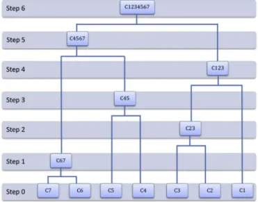
Hierarchical clustering techniques are based on an iterative process. They can be subdivided into two classes: 1/agglomerative methods, which proceed by a series of successive merging of single elements from the initial dataset into groups, as shown schematically inFig. 2if the process goes from Step 0 to 6; 2/divisive methods, which separate the initial set of data successively into smaller groups (the process then goes from Step 6 to 0). Agglomerative hierarchical methods are detailed in the next section.

2.4. Agglomerative hierarchical linkage clustering methods

As depicted inFig. 2, agglomerative hierarchical linkage clustering processes start by placing each element of the input dataset into its own cluster (Step 0). Then, the two elements with the highest similarity, given by Eq.(3), are merged into a single cluster (in the case shown in

Fig. 2, the two most similar elements at the first step are C6 and C7; they are merged into C67). Doing so, the total number of clusters is reduced by one (all the clusters with one element viz. C1-5 which correspond to the initial set and one with two elements C67). The process is then iterated until a prescribed stopping criterion (the total number of clusters for instance) is met. In fact, the procedure illustrated inFig. 2do not need to be done up to Step 6, for which only one cluster remains, but can be stopped at any time providing for instance 3 clusters at Step 3. During the whole clustering process, one of the most important steps is the determination of the most similar clusters. This is not a problem at the first iteration, since Eq.(3)can be used directly. However, at later stages, defining similarities between clusters can become tricky when large groups have to be compared (for merging C67 and C45 into C4567 for instance). Dedicated techniques, known as “linkage” methods, were developed to handle this problem. They are based on the concept of between-cluster similarity (called from now on the linkage function) to select the closest groups of elements at any stage of the clustering process.

The whole grouping procedure illustrated in Fig. 2 can be re-presented by functions called “linkage-based clustering functions”. With these functions, one can formulate unambiguously the whole clustering procedures. The formulations detailed below are inspired from Ref.[21], in which they were formulated in terms of distances. They were adapted to the similarity measures involved in this work. Clusters and linkage functions are defined as:

Definition 1. (clusters and clustering) LetU={ , , , , }u u u1 2 3⋯un be a

dataset ofn elements. We define ′ =P { , , , }C C1 2⋯Cm to be a partition of

the setU into m subsets. The union of all these subsets is U. Each subset is called a cluster.m is the number of clusters. The partitionP is called a′ clustering.

Definition 2. (linkage function) The linkage function is a functionl that evaluates the similarity coefficient S, given by Eq. (3) for single elements, for two clustersC1andC2. It outputs the value of similarity

between these two clusters. It is mathematically defined as: →

l C C( , )1 2 S (5)

whereSrepresents a similarity coefficient between the two clusters. Three linkage functions exist in the literature:

1. Single linkage:

= ∈ ∈

l C CSL( , )1 2 Maxu C u Ca 1,b 2S u u( , )a b (6)

where S u u( , )a b is the similarity coefficient between two single

elements from each cluster,uaandub. 2. Average linkage: =∑ ∈ ∈_⋅ l C CAL( , )1 2 u C u C,_{C C}S u u( , )a b 1 2 a 1 b 2 (7) In Eq.(7), C is used to represent the number of elements in the set C.

3. Complete linkage:

= ∈ ∈

l C CCL( , )1 2 Minu C u Ca 1,b 2S u u( , )a b (8)

The various functions defined by Eqs.(6)–(8)can be interpreted as follows. The single linkage functionlSL associates to the clusters the

value of the highest similarity between two single elements found in each cluster. The average linkage uses the average value of similarities between elements from both clusters to define their similarity. The complete linkage uses the smallest value of similarity between two single elements, one from each cluster.

Definition 3. (linkage-based clustering function) The linkage-based clustering function described here was derived from Ref.[19]. We have changed some of its notations for the sake of clarity and also made the adaptation of this function to the similarity measure. For each possible value of the variablem (defined as an integer between 1 and U), the linkage-based clustering function P U S m( , , ) corresponds to a set of clusters (a partition of the data setU). The number of clusters for this set is equal tom. Some details about this function are provided here:

1. IfP U S m( , , = U), each element of the input data set is inside its own cluster.

As shown in step 0 inFig. 2, the initial set can be presented by this formulation as each element of the input data set is inside its own cluster (U is the set of data investigated,S is the similarity function, mindicates the number of clusters). This initial situation corresponds to the case where cluster number is equal to 7 inFig. 2.

2. For1≤m< U,P U S m( , , ) is constructed by merging two clusters inP U S m( , , +1) which maximizes or minimizes the value of the linkage functionl chosen. This can be illustrated by passing from P U S( , , 6) to P U S( , , 5) in the example ofFig. 2. We choose two clusters inP U S( , , 6) that have the maximum value of l according to Eqs.(6)–(8). These two clusters are then merged together to form a new cluster and we obtain a new set of clusters calledP U S( , , 5). The procedure described above can be formulated mathematically as:

= ∈ + ≠ ≠ ∪ ∪

P U S m( , , ) {C Ci i P U S m( , , 1),Ci C C1, i C2} {C1 C2} (9) such that{C1∪C2} arg= max C C,{ , } P(U,S,m 1)1 2⊆ + l C C S( , , )1 2 where the

argu-ment of the maximum (abbreviatedarg_max) refers to the inputs which create those maximum outputs. Therefore,{C1∪C2}corresponds to the

two clusters whose linkage functionl attains its maximum value no matter which linkage function of Eqs. (6)–(8)is adopted. These two clusters are then merged into one cluster. With other clusters that have not been modified, a new set of clusters is obtained through Eq.(9). Taking the case inFig. 2for example, we have:

= P U S C C C C C C C Step 0 : ( , , 7) { , , , , , , }1 2 3 4 5 6 7 = P U S C C C C C C Step 1 : ( , , 6) { , , , , ,1 2 3 4 5 67} = P U S C C C C C Step 2 : ( , , 5) { ,1 23, , ,4 5 67} = P U S C C C C Step 3 : ( , , 4) { ,1 23, 45, 67} = P U S C C C Step 4 : ( , , 3) { 123, 45, 67} = P U S C C Step 5 : ( , , 2) { 123, 4567} = P U S C Step 6 : ( , , 1) { 1234567}

It should be noticed that another important hierarchical clustering method is the so-called Ward's method[20]. It starts also with each object as its own cluster, as that in linkage methods. The fusion of two clusters is based on the size of an error sum-of-squares criterion. The objective of this method is to minimize the total within-cluster error function in every stage of the whole clustering process. Similar for-mulation as shown in Eqs.(5)–(9)can be derived for the construction of the mathematical clustering function in applying the Ward's method (One can find the detailed derivation inAppendix A).

3. Comparisons between hierarchical clustering methods When applied to functional data, the choice of the linkage function plays a key role in the whole clustering procedure. Indeed, this function drives the clustering process by providing methods to decide which couple of clusters should be merged into a new cluster at any stage of the grouping process. Several studies regarding the performance of distinct linkage functions, such as those defined by Eqs.(6)–(8), can be found in Ref.[19] [22] [23]. All these works are based on discrete and not functional data. Nevertheless, several observations can be made:

1. The single linkage approach performs poorly when compared to other hierarchical clustering methods[19] [23].

2. In general, Ward's method works better than other hierarchical methods when the sizes of different clusters are equal or at least similar. For cases where cluster sizes are not equal, the average linkage method performs the best[19] [22].

3. Generally speaking, the higher the final number of clusters we generate, the better the classification is[19].

In the case of functional data, results from Ref.[18]provide the following conclusions:

1. Ward's method always performs the best except when the data set contains one or two very large groups and several other very small groups; in such cases, the average linkage method performs the best. 2. The complete linkage and single linkage methods cannot be

re-commended for the clustering of functional data.

In this work, the comparisons between different clustering methods are implemented with two criteria proposed in Ref.[24]. The first one is called Homogeneity. It quantifies the uniformity inside a given cluster and is defined as:

∑ ∑

∑

the number of elements inside theith clusters.S u u i( , ( ))i′ represents

the similarity coefficient between the scaling functions of the ′ith ele-ment in theith cluster and the average scaling function of this cluster (represented in Eq. (10-b)). From this criterion, we can tell if each element of the data set is tightly correlated to the core of its cluster or not. The higher the homogeneity, the better the correlation is inside the clusters.

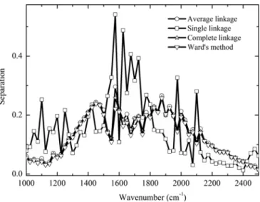
The second criterion is called Separation. It is an indicator of the dissimilarity between different clusters. It is given as:

=∑ ∑ − ∑ ∑ = = = = Sep S u i u j N i N j N i N j {1 [ ( ), ( )]} ( ) ( ) ( ) ( ) i N j N i N j N 1 1 1 1 c c c c (11) whereNcis the number of clusters that exist in the whole set;N i() and

N j() are the number of elements inside theith and jth clusters re-spectively.u i()andu j() are respectively the average scaling functions for theith and jth clusters.S u i u j[ ( ), ( )] is the similarity coefficient between these two mean scaling functions. Hence, the separation in-dicates how much two clusters differ from each other. The higher the separation, the larger the difference between the clusters is.

These two criteria can be used to evaluate the relative efficiency of different clustering techniques. The average linkage, single linkage, complete linkage and Ward's method have been compared in the case of a gaseous mixture composed of 10% H2O and 90% N2in the spectral

interval [1000 cm−1_{, 2500 cm}−1_{]. Mixtures of CO}

2and N2were also

considered. The homogeneity index, separation index and the size of clusters have been investigated and plotted inFigs. 3–5.

1. In all these cases, the single linkage performs the worst according to the criterion set by Eq.(10), i.e. homogeneity, depicted inFig. 3. This can be explained by the sizes of the clusters obtained by ap-plication of the single linkage method. Indeed, we can observe in

Fig. 5that the single linkage always produces one very big cluster, which contains almost 98% of the elements in the dataset. For other clusters, only few isolated elements are present. Hence, the single linkage tends to put all the elements into one big cluster. This will then decrease the homogeneity inside the biggest cluster. And the diversity among the elements inside the biggest cluster has not been sufficiently taken into account.

2. The other three clustering methods share nearly the same perfor-mance from the point of view of homogeneity (seeFig. 3). Only a relative advantage of 0.1% can be found for the Ward's method over the average linkage and complete linkage methods.

3. From the point of view of separation, the single linkage method provides the highest value of separation. The single linkage method takes the biggest similarity between any two elements, one from each cluster, as the similarity between two clusters. Hence, many peripheral points will be included in the main cluster. This will make the cluster less compact compared to clusters generated by the complete linkage and average linkage. However, one advantage of this method is that the peripheral points that are really far away from the core will be identified and isolated. This is the reason why other clusters (except the biggest one) contain only a few points. And this can also explain why the separation of the single method is the highest among all these clustering methods.

4. The separation of the other three clustering methods shares the same performance. Very slightly advantage can be found for the average linkage method over the Ward's and complete linkage methods.

5. The size of clusters for different clustering results has been plotted in Fig. 5(in total 2500 elements, for each discrete wavenumber of the narrow band). Usually, the single linkage method generates one very big cluster and several small clusters; Ward's method leads to clusters of nearly the same size; the average linkage and complete linkage methods are between these two extremes. The average linkage method gives one relatively big cluster (about 1500 ele-ments), several medium size clusters (about 300 elements) and several small clusters (about 30 elements). Ward's method is ap-propriate for cases where the clusters have nearly the equivalent size. The single linkage method is adapted to situations where the whole data set contains only one very big cluster and several iso-lated points. The average linkage method is suitable for cases where one relatively big cluster coexists with several medium and small clusters. The distribution of clusters sizes in the average linkage method is closer to a normal distribution.

The above discussions are based on the investigations in view of some mathematical criteria. The analysis is consistent with the

Fig. 3. Evaluation of different clustering methods according to the homogeneity for the mixture 10%H2O+90%N2at the interval [1000 cm−1, 2500 cm−1].

Fig. 4. Evaluation of different clustering methods according to the separation for the 10% H2O +90%N2at the interval [1000 cm−1, 2500 cm−1].

conclusions drawn by other researchers[18]and discussed previously. A more direct and significant evaluation of these clustering methods consists in assessing their performances for radiative heat transfer computations against reference Line-By-Line (LBL) calculations.

The configuration proposed to compare the clustering techniques consists of a non-uniform two-cell gaseous path with a uniform com-position (10%H2O+90%N2) discretized in two columns at distinct

temperatures (one cold column at 300 K and a hot one at 1000 K). Results are depicted inFig. 6. We can observe that the single linkage method performs the worst, with relative errors up to 50% compared to the LBL reference calculation. This technique provides results as in-accurate as the Ck model (not depicted here). Indeed, the single linkage method produces a single big cluster which is almost the same as the whole dataset. All the other clustering methods provide similar and quite accurate results. The maximum relative errors are 3% for both Ward's and average linkage methods. In Ward's method, all clusters (spectral groups) have the same size which indicates an over-classifi-cation of the dataset. The average linkage method was chosen as the clustering method for further investigations.

4. Estimation of the number of clusters

Choosing a priori the number of clusters is a fundamental issue frequently discussed in cluster analysis. It has a critical effect on the clustering results. In practice, we can rarely build clusters whose ments are exactly the same in all aspects. In most situations, the ele-ments in the same cluster share some major characteristics, but a little difference in some less important features can also be found among them. If the number of clusters is chosen too big, the singularity of each cluster will be too outstanding such that it conceals some important characteristics shared by different clusters. One extreme example can be found inFig. 2when the cluster number is chosen to be 6. In this case, each element is its own cluster and the clustering technique has no effect on the classification. If the number of clusters is chosen too small, the number of elements contained in the clusters will be very big. In this case, we will find the division of the whole data set to be insufficient and the elements in each cluster may be over mixed. Therefore, we need to choose an appropriate number of clusters, neither too big, nor too small. Unfortunately, due to the high complexity of real data sets, there is no convincingly acceptable solution to this problem. In practice, the number of clusters is usually specified by the investigator a priori. In this Section, we will make a brief discussion about the estimation of cluster number from several different points of view.

Firstly, from the view of clustering technique itself, a better

classification can be achieved if we increase the number of clusters. An extreme case is to put each element of the data set inside its own cluster. In this case, the absolute uniformity is maintained inside each cluster. However, a better classification can be achieved by increasing the number of clusters but this will not guarantee better simulation results when this number exceeds a certain limit.Fig. 7andFig. 8show the relative error of MSCk model compared to the line by line bench-mark calculation for the same case as inFig. 6. The number of clusters investigated is 9, 25, 50 inFig. 7and 50, 100, 300 inFig. 8. FromFig. 7, we can observe that the performance of the average linkage clustering method increases with the number of clusters. However, inFig. 8, an evident loss of accuracy is observed if we increase further the number of clusters from 50 to 100 and from 100 to 300. This can be explained by the fact that high number of clusters are associated with large numbers of small clusters (defined in this work as clusters whose size is smaller than 15): the proportion of clusters whose size is less than 15 increases significantly as we augment the number of clusters (shown inFig. 9). In this case, most of the error of the model is due to the fact that we try to represent these small clusters using k-distributions, which is question-able for very small spectral intervals.

Secondly, from a mathematical view, several statistical criteria have been proposed to determine the best number of cluster. These criteria are usually based on the concepts of within-cluster and

between-Fig. 6. Relative errors between the results of different clustering methods and that of the line by line calculation.

Fig. 7. The same calculation as inFig. 6by using the average linkage method of 9 clusters, 25 clusters and 50 clusters.

Fig. 8. The same calculation as inFig. 6by using the average linkage method of 50 clusters, 100 clusters and 300 clusters.

clusters variance[25]. They try to identify the best number of clusters which permits that “the elements are most similar inside a given group” and “the most different with elements in other groups”. This looks like to be a powerful tool to make a serious decision. An investigation of such criteria has been made. In the literature, we can find about 30 different criteria for the determination of the number of clusters. Among all these criteria, the CH[26]and Duda[27]indexes are the two best according to the study of Milligan and Copper [28]. More information about these two criteria can be found inAppendix B. After an investigation (shown inFig. 10) of these two criteria, we found that each criterion proposes different values and there is no superiority of one criterion over another. In addition, the appropriate number of clusters proposed is not a fixed value for all intervals. It changes from one interval to another. This will increase the complexity of the whole clustering programming. Furthermore, the number proposed is gen-erally smaller than 9. After investigations of the clustering effect in the radiation calculation performed inFig. 7, we find that the calculation accuracy has an increasing tendency as we augment the number of clusters from 9 to 25. Hence, we cannot decide the number of clusters only according to these statistical criteria.

Thirdly, from the view of accuracy, letting the investigator decide the appropriate number of clusters brings some freedom to adjust the accuracy of the simulation compared to the LBL results. Nevertheless, a

specific attention should be taken about the existence of extremely small groups. When the number of clusters is increased, the possibilities for the appearance of these extremely small groups are greatly in-creased. One solution to this problem is using the line by line method in these extremely small groups. All these operations will undoubtedly make the programming more complicated. In general, the investigator needs to find a good compromise between the advantages and limita-tions mentioned above in order to find the appropriate number of clusters. As shown inFigs. 7 and 8, the model accuracy increases with increasing number of clusters, from 9 to 25. The relative error keeps a nearly constant value (around 3%) between 25 and 100. For numbers higher than 100, more errors emerge. Therefore, setting the number of clusters at 25 at atmospheric pressure is an appropriate choice. At higher pressures, this number can be decreased as the spectral dynamics of absorption coefficient is strongly reduced compared to low pressures. For high pressure calculations, two clusters were chosen. Results for these models will be provided later in this paper.

5. Application

The principle of the multispectral framework (MSCk) is extensively detailed in Refs.[1,2]where several validations against 0D and 1D case studies at atmospheric pressure can be found (here we provide a vali-dation of this model in the oxy-fuel combustion case inAppendix. C). In the present work, the multispectral technique is applied to 1D and 3D configurations at high pressure (3 atm), encountered in particular for aeronautic applications. In contrast to previous work (where up to 25 clusters were considered for each narrowband), only two clusters are generated here, following the scheme of hierarchical average linkage introduced previously. The results obtained with this approach are compared to standard correlated k-distributions and to reference line-by-line models. The efficiency, the accuracy and the adaptability to complex configurations of this model are discussed at the end of the section.

5.1. Model parameters

The three considered models result from a unique precomputation of line-by-line spectra at 0.01 cm−1 _{resolution. These spectra were}

generated using the CDSD-4000[29]and HITEMP-2010[30] spectro-scopic databases, respectively to account for CO2and H2O species. The

resulting spectra dataset, produced for P = 3atm, covers the tempera-ture range from 300 K to 5000 K (with 100 K steps) and the mole-fractions range from 0.01 to 1 (with steps varying between 0.09 and 0.2). The spectroscopic assumptions used for this LBL production are those used in Ref.[31]with the exception of sub-lorentzian corrections that have been neglected.

In addition to their role of reference, the LBL spectra were employed to produce Ck and MSCk models. The Ck model used in the present work was built for 25 cm−1_{narrowbands using 7 values of absorption}

coefficients which comply with Gauss-Legendre quadrature. The MSCk database was also computed considering 25 cm−1 _{narrowbands. For}

each band, each thermophysical set and each species, two clusters of wavenumbers were built according to the hierarchical average linkage approach. In each group, 7 values of absorption coefficient were con-sidered as for standard Ck approach. A weight w was also assigned to each cluster. Starting from LBL spectra, it is defined as the ratio of the number of wavenumbers linked to the considered cluster over the total number of wavenumbers of its narrowband.

5.2. One-dimensional configurations

The first four test cases involve H2O/N2 mixtures in

one-dimen-sional geometries composed of gaseous media surrounded by two walls. These configurations are respectively taken from Ref.[32]for case C1 and from Ref.[33]for cases C2 to C4.

Fig. 9. Proportion of the clusters whose size is lower than 15 for the average linkage clustering method of different number of clusters (9, 25, 50, 100, 300).

Case C1, is composed of an isothermal mixture of 50% H2O at

T = 1500 K. Both walls are assumed isothermal:Tw x, 0= =1200K and =

=

Tw x, 1 600K, gray and partially reflecting – of emissivityε 0.6. For= cases C2 and C3 the mole-fraction of H2O is set at 10% and the

tem-perature profile is assumed as a parabolic function given by:

= − ⎛

⎝ − ⎞⎠ + T x( ) 4(Tw T xc) _L 0.5 Tc

2

(12) where L is the distance between the walls surrounding the medium;Tw

andTc are respectively the temperature of both walls and the

tem-perature at the center of the medium atx L/2. The walls are assumed= as gray, with an emissivity ε 0.5= . Temperatures are defined as

Tw= 2500 K andTc= 500 K for case C2 and are interchanged for case

C3 (Tc= 2500 K andTw= 500 K). The last case: C4 - known to be very

sensitive to the accuracy of the spectral model - is composed of a 10% H2O gaseous mixture. Its temperature is equal to the walls temperature Tw= 500 K in the whole medium, except in a central region of 10 cm

width, where a triangular profile is assumed, reaching a maximum valueTc= 2500 K atx L/2.=

For each case, the wall radiative fluxes and the divergence of flux were computed in several points of the geometry. These simulations were performed using the semi-analytical resolution of the RTE de-scribed in Ref.[34].

Figs. 11–13depict, for cases C1 to C3, the divergence of radiative flux obtained with LBL, Ck and MSCk2 models along the x-axis.Fig. 14, represents the wall fluxes as a function of the distance L for case C4. The relative differences between approximated models and LBL solutions are also given for each figure.

For all four test cases, the multispectral framework leads to more accurate results than standard Ck models. Only two clusters are suffi-cient to divide the error of Ck, by an average factor about 2. In terms of computation time, the semi-analytical nature of the approach used here to solve the RTE drives to simulation times nearly proportional to the number of considered groups (here MSCk2 is twice more expensive than Ck for a doubled accuracy).

5.3. Three-dimensional configuration

The same comparative study was conducted for a three-dimensional enclosure. This configuration, taken from case tests proposed in Ref. [35] [36], has a cylindrical geometry of lengthL=1.2 and of radiusm

=

R 0.3 . A gaseous mixture composed of COm 2, H2O and N2at a

pres-sure of P=3atm is considered inside this chamber. Boundaries are assumed as black surfaces (ε 1= ). Their temperature are set as

=

Tw 800Kexcept for the surface located atx=1.2 wherem Tw=300K.

The fields of temperature and mole fractions are axisymmetric and are given by the following set of analytical functions:

⎧ ⎨ ⎪ ⎪ ⎩ ⎪ ⎪ = + − = − − − = − − −

(

)

(

)

( )( )

(

) ( )

(

) (

)

withr= y2+z2_{. These properties fields are depicted inFig. 15.}

The RTE resolution was performed using Monte Carlo methods, chosen here for their high ability to treat complex geometries. Three spectral models were considered: Line-by-line, Ck and MSCk2. In order to prevent the use of mesh - which can be very expensive to manage in terms of computation time - a null-collision strategy has been adopted for the three considered models. Such an approach, largely described in Ref.[37] [38], requires the definition of an arbitrary extinction coef-ficient greater than the real one for all wavenumbers (or bands) and thermophysical sets of properties (temperature, pressure and mole fractions). For efficiency purposes, a maximum value of absorption coefficient was here identified for each narrowband of 25 cm−1_width,

via a lookup of the line-by-line database described previously. Null-collision Monte-Carlo algorithms are fully adapted to the use of correlated k-distributions. Its extension to MSCk only requires a minor modification of the algorithmic structure. With Ck, the spectral in-tegration is done by sampling a narrowband and a value g of the cu-mulative k-distribution at the beginning of each independent Monte Carlo realization (see Ref.[38]for more details). With MSCk, a third step is required to perform this integration: the sampling of a group according to the weights w precomputed during the database produc-tion. These small changes were applied in the EDStaR development environment[39](dedicated to the stochastic simulation of radiative transfer in real geometries using computer graphics libraries) from which computations were performed.

Results are displayed inFigs. 16 and 17where the divergences of radiative flux are represented for different locations inside the en-closure: along the axis of symmetry x (with r = 0) inFig. 16and along a radial direction at x=L/2 inFig. 17. The relative differences between approximate models (Ck and MSCk2) and reference LBL computation are also depicted with their interval of confidence (proper to Monte-Carlo methods, given here for 108_{independent realizations).}

As for 1D configurations, the results obtained with MSCk2 are nearly twice more accurate than with Ck. However, in the present case,

Fig. 11. Divergence of the radiative flux computed along the x-axis in the configuration C1 (isothermal gaseous H2O/N2mixture surrounded

by reflecting walls). Top: Line-by-Line computation; bottom: relative difference between model (Ck and MSCk2) and LBL calculations.

the spectral integration was stochastically performed and similar computation times were observed for both models (for equal standard deviations). Indeed the clustering technique does not add supplemen-tary variance to the estimate of fluxes by comparison to Ck approaches and the same number of independent Monte Carlo realizations are re-quired to reach equivalent standard deviations.

5.4. Discussion

At high pressure, the correlation assumption is generally less pre-judicial than at lower pressures (one can compareFig. 14toFig. 7of reference[8]). However, even in such cases, Ck models can show im-portant discrepancies by comparison to LBL results (almost 20% for the case C4). In the five test cases addressed in this work, the proposed 2 clusters – MSCk2 model, defined according to the hierarchical average linkage, increases the accuracy of results by a factor about 2.

This qualitative refinement weakly affects computation time. As shown here, this increase is essentially dependent on the RTE method of resolution. In the worst cases: when a deterministic spectral integration is performed, the increase of computation time is proportional to the number of groups. Such a linear relationship between accuracy and time consumption is rather rare when refining spectral models: highly

Fig. 12. Divergence of the radiative flux computed along the x-axis in the configuration C2 (gaseous H2O/N2 mixture with a parabolic

temperature profile, Tc < Tw). Top: Line-by-Line computation;

bottom: relative difference between model (Ck and MSCk2) and LBL calculations.

Fig. 13. Divergence of the radiative flux computed along the x-axis in the configuration C3 (gaseous H2O/N2mixture with a parabolic

temperature profile, Tc > Tw). Top: Line-by-Line computation;

bottom: relative difference between mode (Ck and MSCk2) and LBL calculations.

Fig. 14. Wall net flux versus distance between cold walls for the configuration C4 (gas-eous H2O/N2mixture with a 10 cm width triangular profile of temperature located in cold

medium). Top: Line-by-Line computation; bottom: relative difference between model (Ck and MSCk2) and LBL calculations.

non-linear evolutions are more frequently observed.

Moreover, when the spectral integration is performed in a stochastic way, as in case C5, the effects on the computation become negligible since no additionally variability is induced by the clustering technique itself. Furthermore, as for Ck, one can take advantage of the simple structure of MSCk (by comparison to LBL) to easily propose variance reduction techniques[40] [41]that would substantially accelerate the computation process.

Finally, this model was shown to be perfectly adapted to 3D Monte Carlo solvers and requires only few algorithmic changes if correlated k-distributions are already handled. This can open the door to fast and accurate simulation tools for complex configurations, including for in-stance scattering medium or complex geometries.

6. Conclusion

This paper has been dedicated for the presentation about the prin-ciple issues of applying Functional Data Analysis (FDA) in the MSCk model. In the MSCk model developed in previous work, the FDA method is applied in order to classify wavenumbers whose absorption coefficients have similar behaviors as function of the thermophysical conditions. As a result of this classification, the correlation assumption inside each of these groups (clusters) can be better satisfied. The steps for the application of FDA method have been detailed.

Firstly, spectral data are used for the construction of scaling func-tions. A mathematical formulation of the scaling function is applied in this work.

Secondly, the agglomerative hierarchical average linkage method is chosen as the clustering method. Several investigations from the aspect of statistical criteria and a practical radiation calculation have been

performed to make this choice. Among all the clustering methods stu-died (average linkage, single linkage, complete linkage and Ward's method), the single linkage performs the worst because this method usually generates a very big cluster and several extremely small clusters which contain only several isolated elements. This kind of clustering makes the whole classification insufficient. The diversity inside the data set studied has not been sufficiently excavated. The other three clus-tering methods perform all very well, with only slightly difference be-tween them. The main difference among them exists in the size of clusters. The Ward's method tends to generate clusters of nearly equivalent size. Contrary, the average linkage method generates a re-latively big cluster, several medium clusters and some rere-latively small clusters. As we assume that the correlation assumption corresponds to the cluster-size distribution of the average linkage method, this method is hence chosen for the further calculations.

The average linkage algorithm starts by putting every single ele-ment of the input data set as its own cluster. Then, it gradually merges the “closest” clusters until the stopping criterion is met. Usually, this process is stopped when an assigned number of clusters is attained. The choice of the number of clusters has an important impact on the clus-tering results. In general, investigators need to find a good balance between all the advantages and limitations mentioned in Section4in order to find an appropriate value for the cluster number. At the end of the process, the elements in the clusters correspond to spectral intervals that are associated to similar scaling functions. Over these intervals, gas spectra are mostly scaled. Nevertheless, as the so-called scaled-k model [7]has been relatively poorly studied in the literature, we have chosen to treat gas spectra as correlated over the intervals. The resulting multi-spectral correlated-k distribution model was applied to several test-cases from the definition of two clusters. This approach shown to be

Fig. 15. Fields of temperature, H2O, and CO2mole-fractions for the axisymmetric configuration of test case C5. Fields are described as functions of transversal (x) and radial (r) positions.

Fig. 16. Divergence of the radiative flux computed along the x-axis in the configuration C5 (gaseous H2O/CO2/N2mixture) along the

axis of symmetry x. Top: Line-by-Line computation; bottom: relative difference between model (Ck and MSCk2) and LBL calculations.

more reliable than standard Ck models with comparable computation times and fully compliant with complex 3D geometries and Monte Carlo algorithms.

Acknowledgments

This work was supported by the French National Research Agency

under the grant ANR-12-BS09-0018 SMART-LECT.

Appendix A. Formulation of the clustering function for Ward's method

The Ward's method[20]is based on the idea of minimizing the increase in the total within-cluster error sum of squares, E, formulated as:

∑

∑ ∑

u ϕk _q (1/ )nk lnk1u ϕkl _q defines the mean of the kth cluster for the thermophysical conditionϕq, ⎜⎛ ⎟

⎝ ⎞ ⎠

u ϕkl _q is the value of the qth variable

(q =1, …, pq) for the lth object (l = 1, …,nk) in the kth cluster (k = 1, …,K). We further defineE C C( , )1 2 as the total within-cluster error sum of

squares of the new set of clusters for which clusterC1and clusterC2are merged into one cluster.

With the above definition of the Ward's method, the formulation of the clustering function of the Ward's method can be derived in a similar way as the linkage method as following:

1. IfP U S m( , , = U), each element of the input data set is inside its own cluster.

2. For1≤m< U,P U S m( , , ) is constructed by merging two clusters inP U S m( , , +1) which minimizes the total within-cluster error sum of squares in Eq. (A.1). The procedure can be formulated mathematically as:

= ∈ + ≠ ≠ ∪ ∪

P U S m( , , ) {C Ci i P U S m( , , 1),Ci C C1, i C2} {C1 C2} (A.3)

such that{C1∪C2} arg= min,{ , } P(U,S,m 1)C C_{1 2}⊆ + E C C( , )1 2 where the argument of the minimum (abbreviatedargmin) refers to the inputs which create those

minimum outputs. Therefore,{C1∪C2}corresponds to the two clusters which can minimize the total within-cluster error sum of squares. These two

clusters are then merged into one cluster.

With other clusters that have not been modified, a new set of clusters is obtained. Appendix B. Definition of the CH and Duda indexes

The Calinski-Harabasz index[26]is defined as:

= × −

−

CH SSB

SSW N kk 1 (B.1)

where SSW is the overall within-cluster variance, SSB is the overall between-cluster variance, k is the number of clusters, and N is the number of all the individual elements.Where

Fig. 17. Divergence of the radiative flux computed along the x-axis in the configuration C5 (gaseous H2O/CO2/N2 mixture)

along the axis of symmetry x. Top: Line-by-Line computation; bottom: relative difference between model (Ck and MSCk2) and LBL calculations.

∑ ∑ ∑

u ϕk _q (1/ )nk lnk1u ϕkl _q defines the mean of the kth cluster for the thermophysical condition ϕq, ⎜⎛ ⎟

⎝ ⎞ ⎠

u ϕkl _q is the value of the qth variable

(q = 1, …, pq) for the lth object (l = 1, …,nk) in the kth cluster (k = 1, …,K).

∑ ∑

u ϕk _q (1/ )nk lnk1u ϕkl _q defines the mean of the kth cluster for the thermophysical conditionϕq, ⎜⎛ ⎟ ⎜ ⎟

⎝ ⎞ ⎠= ∑ ⎛ ⎝ ⎞ ⎠ = u ϕ_q (1/ )N _lN u ϕ l _q 1 defines

the mean of the whole N elements studied for the thermophysical condition ϕ_q.

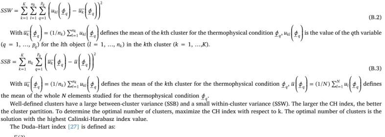
Well-defined clusters have a large between-cluster variance (SSB) and a small within-cluster variance (SSW). The larger the CH index, the better the cluster partition. To determine the optimal number of clusters, maximize the CH index with respect to k. The optimal number of clusters is the solution with the highest Calinski-Harabasz index value.

The Duda–Hart index[27]is defined as: =

E E_E(2)_{(1) (B.4)}

where E(1) is the sum of squared errors within the group that is to be divided. E(2) is the sum of squared errors in the two resulting subgroups. The formulation of the sum of squared errors within the group can be found in Eq.(A.2). Large values of the Duda–Hart index indicate distinct cluster structure. Small values indicate less clearly defined cluster structure. The Duda–Hart index requires hierarchical clustering information. It needs to know at each level of the hierarchy which group is to be split and how. The Duda–Hart index is also local because the only information used comes from the group's being split. The information in the rest of the groups does not enter the computation.

Appendix C. Validation of the MSCk model in an oxy-fuel combustion case

The basic configuration of the case discussed here are taken from the article of CHU[43]. It involves a 1D parallel plate geometry of black and cold walls. The length of the plate is set at 0.035 m. A mixture gas of CO2and H2O at atmospheric pressure is present in this case. The corresponding

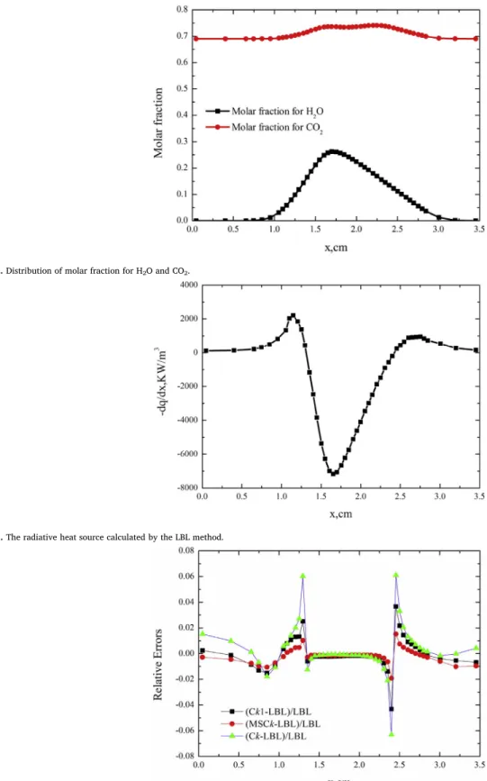
temperature distribution and molar fractions of these two gases are drawn inFigure D.1andFigure D.2.

Fig. D.2. Distribution of molar fraction for H2O and CO2.

Fig. D.3. The radiative heat source calculated by the LBL method.

Fig. D.4. Relative errors of different models in comparison with the LBL benchmark results.

This configuration is usually used for the simulation of oxy-fuel flame with dry flue gas recirculation. The spectra used in this case are from reference[14]. The discrete ordinate method (DOM) along with the T7angular discretization is applied for all the calculations, more details about

this method can be found in Ref.[44]. We use in this case 65 non uniform grids in order to better capture the non-uniformity of temperature distribution in this case. The models studied in this case are respectively: the Line-by-Line model (LBL), Ck1 model (narrow band interval equals to 1 cm−1_{), Ck model (narrow band interval equals to 25 cm}−1_{), and the MSCk model (25 clusters generated in the 25 cm}−1_{narrow band). The}

radiative heat source calculated by the LBL method is shown inFigure D.3. The relative errors of the Ck, Ck1 and MSCk models when compared to the LBL benchmark results are demonstrated inFigure D.4. FromFigure D.4, we can find that the MSCk model is more accurate than the Ck and Ck1 model, with the maximum relative error 1% for the MSCk model, 4% for the Ck1 model and 6% for the Ck model. Notice that, the MSCk model and

Ck1 model share nearly the same computational cost. In addition to the validations already made in Refs.[1]and[2], the results of this case add another evidence to the conclusion that the MSCk is more accurate than the Ck model.

References

[1] F. Andre, L. Hou, M. Roger, R. Vaillon, The multispectral gas radiation modeling: a new theoretical framework based on a multidimensional approach to k-distribution methods, J Quantitative Spectrosc Radiat Transf 147 (2014) 178–195.

[2] F. Andre, L. Hou, V.P. Solovjov, An exact formulation of k-distribution methods in non-uniform gaseous media and its approximate treatment within the Multi-Spectral framework, J Phys Conf Ser 676 (1) (2016).

[3] E.P. Keramida, H.H. Liakos, M.A. Founti, N.C. Markatos, Radiative heat transfer in natural gas-fired furnaces, Int J Heat Mass Transf 43 (2000) 1801–1809. [4] P.J. Stuttaford, P. Rubini, Assessment of a radiative heat transfer model for gas

turbine combustor preliminary design, J Propuls Power 14 (1998) 66–73. [5] C. Caliot, et al., Remote sensing of high temperature H2O–CO2–CO mixture with a

Correlatedk-distribution fictitious gas method and the single-mixture gas as-sumption, J Quantitative Spectrosc Radiat Transf 102 (2006) 304–315. [6] J.F. Sacadura, Radiative heat transfer in fire safety science, J Quantitative Spectrosc

Radiat Transf 93 (2005) 5–24.

[7] H. Chu, F. Liu, H. Zhou, Calculations of gas radiation heat transfer in a two-di-mensional rectangular enclosure using the line-by-line approach and the statistical narrow-band correlated-k model, Int J Therm Sci 59 (2012) 66–74.

[8] J.L. Consalvi, F. Liu, Radiative heat transfer in the core of axisymmetric pool fires – I: evaluation of approximate radiative property models, Int J Therm Sci 84 (2014) 104–177.

[9] M.F. Modest, Radiative heat transfer, second ed., Academic Press, New York, 2003. [10] J.O. Ramsay, B.W. Silverman, Functional data analysis, second ed., Springer Series

in Statistics, 2009.

[11] R. West, D. Crisp, L. Chen, Mapping transformations for broadband atmospheric radiation calculations, J Quantitative Spectrosc Radiat Transf 43 (3) (1990) 191–199.

[12] H. Zhang, M.F. Modest, A multi-scale full-spectrum correlated-k distribution for radiative heat transfer in inhomogeneous gas mixtures, J Quantitative Spectrosc Radiat Transf 73 (2) (2002) 349–360.

[13] P. Rivière, A. Soufiani, Correlated-kand fictitious gas methods for H2O near 2.7 µm, J Quantitative Spectrosc Radiat Transf 48 (1992) 187–203.

[14] L. Hou, Simulation study of the Multi-Spectral Correlated-k distribution model, Ph.D. thesis Institut National des Sciences Appliquées de Lyon, Lyon, France, 2015. [15] A.A. Lacis, A description of the correlated-k distribution method for modeling

nongray gaseous absorption, thermal emission, and multiple scattering in vertically inhomogeneous atmospheres, J Geophys Res 96 (D5) (1991) 9027–9063. [16] Q. Fu, K.N. Liou, On the correlatedk-distribution method for radiative transfer in

nonuniform atmospheres, J Atmos Sci 49 (1992) 2139–2156.

[17] R.M. Goody, Y.L. Yung, Atmospheric radiation, Oxford Univ. Press, New York, 1989.

[18] L. Ferreira, B.D. Hitchcock, A comparison of hierarchical methods for clustering functional data, Commun Stat. Simul Comput 38 (2009) 1925–1949.

[19] B.S. Everitt, S. Landau, M. Leese, D. Stahl, Cluster analysis, fifth ed., John Wiley and Sons, 2010.

[20] J.H. Ward, Hierarchical grouping to optimize an objective function, J Am Stat Assoc 58 (1963) 236–244.

[21] M. Ackerman, S. Ben-David, D. Loker, Characterization of linkage-based clustering, COLT (2010) 270–281.

[22] S. Hands, B. Everitt, A Monte Carlo study of the recovery of cluster structure in binary data by hierarchical clustering techniques, Multivar Behav Res 22 (1987) 235–243.

[23] F.K. Kuiper, L. Fisher, A Monte Carlo comparison of six clustering procedures,

Biometrics 31 (1975) 777–783.

[24]R. Shamir, R. Sharan, Algorithmic approaches to clustering gene expression data. Current topics in Computational Molecular Biology, MIT presss, boston, MA, 2001. [25]G. Chen, S.A. Jaradat, N. Banerjee, T.S. Tanaka, M.S.H. Ko, M.Q. Zhang, Evaluation and comparison of clustering algorithms in analyzing es cell gene expression data, Stat Sin 12 (2002) 241–262.

[26]T. Calinski, J. Harabasz, A dendrite method for cluster analysis, Commun Statics-Theory methods 3 (1974) 1–27.

[27]R.O. Duda, P.E. Hart, Pattern classification and scene analysis, John Wiley & Sons, New York, 1973.

[28]G.W. Milligan, M.C. Copper, An examination of procedures for determining the number of clusters in a data set, Phychometrika 50 (1985) 159–179.

[29]S.A. Tashkun, V.I. Perevalov, CDSD-4000: high resolution, high temperature carbon dioxide spectroscopic databank, J Quantitative Spectrosc Radiat Transf 112 (2011) 1403–1410.

[30]L.S. Rothman, I.E. Gordon, R.J. Barber, H. Dothe, R.R. Gamache, A. Goldman, et al., HITEMP, the high-temperature molecular spectroscopic database, J Quantitative Spectrosc Radiat Transf 111 (2010) 2139–2150.

[31]Ph Rivière, A. Soufiani, Updated band model parameters for H2O, CO2, CH4 and CO radiation at high temperature, Int J Heat Mass Transf 55 (2012) 3349–3358. [32]M.K. Denison, A spectral line based weighted sum of gray gases model for arbitrary

RTE solvers, (1994) [Ph.D. thesis].

[33]L. Pierrot, A. Soufiani, J. Taine, Accuracy of narrow band and global models for radiative transfer in H2O, CO2 and H2O-CO2 mixtures at high temperature, J Quantitative Spectrosc Radiat Transf 62 (1999) 523–548.

[34]V.P. Solovjov, B.W. Webb, Multilayer modeling of radiative transfer by SLW and CW methods in non-isothermal gaseous medium, J Quantitative Spectrosc Radiat Transf 109 (2008) 245–257.

[35]P.J. Coelho, P. Perez, M. El Hafi, Benchmark numerical solutions for radiative heat transfer in two-dimensional aximmetric enclosures with nongray sooting media, Numer Heat Transf Part B Fundam 43 (2003) 37–41.

[36]P. Perez, M. El Hafi, P.J. Coelho, R. Fournier, Accurate solutions for radiative heat transfer in two-dimensional axisymmetric enclosures with gas radiation and re-flective surfaces, Numer Heat Transf Part B Fundam 47 (2004) 39–63. [37]M. Galtier, S. Blanco, C. Caliot, C. Coustet, J. Dauchet, M. El Hafi, et al., Integral

formulation of null-collision Monte Carlo algorithms, J Quantitative Spectrosc Radiat Transf 125 (2013) 57–68.

[38]V. Eymet, D. Poitou, M. Galtier, M. El Hafi, G. Terrée, R. Fournier, Null-collision meshless Monte-Carlo—application to the validation of fast radiative transfer sol-vers embedded in combustion simulators, J Quantitative Spectrosc Radiat Transf 129 (2013) 145–157.

[39] StarWest, EDStaR, (2016)http://edstar.lmd.jussieu.fr/.

[40]W.L. Dunn, J.K. Shultis, Exploring Monte Carlo methods, Elsevier, 2012. [41]J. Delatorre, G. Baud, J.J. Bézian, S. Blanco, C. Caliot, J.F. Cornet, et al., Monte

Carlo advances and concentrated solar applications, Sol Energy 103 (2014) 653–681.

[42]T. Kanungo, D.M. Mount, N. Netanyahu, C. Piatko, R. Silverman, The efficient K-means clustering algorithm: analysis and implementation, IEEE Trans Pattern Anal Mach Intell 24 (7) (2002) 881–892.

[43]H. Chu, M. Gu, C. Jean-Louis, F. Liu, Effects of total pressure on non-grey gas ra-diation transfer in oxy-fuel combustion using the LBL, SNB, SNBCK,WSGG, and FSCK methods, J Quantitative Spectrosc Radiat Transf 172 (2016) 24–35. [44]P.J. Coelho, Numerical simulation of radiative heat transfer from non-gray gases in

three-dimensional enclosures, J Quantitative Spectrosc Radiat Transf 74 (2002) 307–328.