HAL Id: hal-02893252
https://hal.telecom-paris.fr/hal-02893252
Submitted on 8 Jul 2020
HAL is a multi-disciplinary open access
archive for the deposit and dissemination of
sci-entific research documents, whether they are
pub-lished or not. The documents may come from
teaching and research institutions in France or
abroad, or from public or private research centers.
L’archive ouverte pluridisciplinaire HAL, est
destinée au dépôt et à la diffusion de documents
scientifiques de niveau recherche, publiés ou non,
émanant des établissements d’enseignement et de
recherche français ou étrangers, des laboratoires
publics ou privés.
Sébastien Mazaré, Jean-Luc Dugelay, Renaud Pacalet
To cite this version:
Sébastien Mazaré, Jean-Luc Dugelay, Renaud Pacalet.
USING GPU FOR FAST
BLOCK-MATCHING. 14th European Signal Processing Conference / EUSIPCO’06, Sep 2006, Florence, Italy.
�hal-02893252�
USING GPU FOR FAST BLOCK-MATCHING
S´ebastien Mazar´e, Jean-Luc Dugelay, and Renaud Pacalet
Multimedia Department, Eurecom Institute and LabSoc, ENST, 2229, route des Cretes, 06560 Sophia-Antipolis, FRANCE email: {mazare, dugelay}@eurecom.fr, [email protected] ABSTRACT
On the one hand, basic PCs include by default more and more powerful GPU (Graphics Processing Unit) that some-times even outperforms CPU (Central Processing Unit) for some specific tasks. On the other hand, video processing are more and more useful and required for numerous emerging services and applications but is often too computational ex-pensive to reach real time. Within the context of GPGPU (General Purpose GPU), we propose in this paper a possible implementation of a block-matching algorithm. Some signif-icant results are obtained in terms of acceleration and qual-ity. Based on our experiments on Block-Matching within the context of video compression, we finally underline some ex-isting limitations of using GPUs beyond graphics for image and video processing even if this concept remains attractive.
1. INTRODUCTION
Originally dedicated to 3D graphics, Graphical Processing Units (GPUs) became more and more powerful, evolving faster than moore’s law. This evolution has been made possi-ble by a market lead by video games, where more and more impressive visual effects are required. In order to allow fast and customizable real-time rendering, some sections of these chips became programmable, offering several dedicated and parallelized processors. An optimal and efficient use of all these processors provides a peak performance in floating-point operations that is far above CPUs.
In this paper, we intend to use this computational power for more generic applications, such as Digital Signal Process-ing Applications. Block-matchProcess-ing is a very interestProcess-ing exam-ple to imexam-plement on GPU: this task has already been widely studied to reduce its complexity while keeping good results, in particular by using sophisticated predictors[1, 2, 3, 4]. In some other words, GPU can be seen as a new element to con-sider when looking for optimization of image and video pro-cessing tasks and a possible source to save execution time. Besides utilization of multiprocessors or clusters, dedicated hardware (e.g. DSP), or/and algorithmic simplications, GPU may offer new possibilities associated with differents pros and cons.
But this approach requires a knowledge of GPU architecture and programming interfaces. A quite restricted set of highly-parallelizable tasks may be implemented. We decided to study a Block-Matching motion estimation algorithm. Once implemented on the GPU, it has been used from a software MPEG-encoder, in order to validate the Digital Signal Co-processor concept and to compare algorithmical qualities.
2. GRAPHICS HARDWARE AS A DIGITAL SIGNAL COPROCESSOR
2.1 The Graphic Pipeline
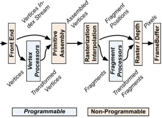
Modern Graphics Hardware may be seen as an output device that processes high-level graphical commands sent from the main processor[7]. These commands are issued using a soft-ware Graphical or 3D API (Applications Programming In-terface), usually OpenGL or Direct3D. The whole Graphical Processor is designed in order to optimize 3D graphics, 2D being still possible as a particular case of 3D. The following dataflow is illustrated by figure 1.
1. In the common case, all raw images needed during the processing are sent to the GPU and stored in its texture memory. Then a geometrical and command flow is sent to the GPU. This flow contains all information on how the rendering shall be performed, and all geometrical in-formation, represented by vertices.
2. Then, a first set of parallel and programmable
proces-sors, theVertex Processors, transforms all characteristic
points of the scene, usually performing a projection from the absolute 3D world described in the CPU to the tar-geted point of view. This way, any important point has its definitive on-screen position set. Input and output struc-tures are both Vertices.
3. These transformed vertices are then assembled in geo-metric primitives, usually in triangles, as specified by the API. The set of vertex indices that belong to the same ob-ject cannot be modified in the GPU. This leads to poly-gons, lines or simple points. The next step is the ras-terization, where any possible future pixel in the object, called a fragment, is generated at its definitive location. All values belonging to these fragments, e.g. color, tex-ture coordinates, are interpolated from the values belong-ing to each vertex of the object.
4. Another set of programmable processors, theFragment
Processors, executes a short section of code on each fragment, performing all texture memory accesses ac-cordingly to this code. This code is usually designed to compute each pixel color from textures, lighting informa-tion, transparency...
5. Finally, the depth is compared to the Z-Buffer to discard any fragment too far or behind an existing pixel. On the other fragments, some optional processing is performed and pixels are updated in the framebuffer, which is the memory section displayed on-screen.
This highly dedicated hardware has an incredible power be-hind it. We used the nVidia 6800GT: It provides six Vertex Processors and sixteen Fragment Processors. Any processor is able to perform the common operations in dimension four and in 32 bits floating point precision in a single cycle, even
Rasterization Interpolation Front End Raster / Depth FrameBuffer Primitive Assembly Fragment Processors V ertex Processors Programmable Non-Programmable Vertices In -dex Stream Vertices Transformed Vertices Assembled Vertices Fragments Fragment Positions Transformed Fragments Pixels
Figure 1: The Graphical Pipeline
two per cycles in particular cases. Memory accesses from the fragment processors are cached in an optimized way, and it is possible to access memory from the vertex processors despite a higher cost. Running at 450 MHz, this leads to a peak performance far above classical CPUs. This is why it is really interesting to use the GPU as a coprocessor for some tasks that fit in it. These processors can be programmed in the Cg language and controlled with the OpenGL API. 2.2 General Purpose and Digital Processing Program-ming
This hardware as it has been described is useless besides the case of real-time graphics. In fact, it is possible to read back the framebuffer from the CPU, thereby allowing a feedback of the processing done. The API provides a set of extensions that enables rendering to a texture instead of the framebuffer, offering the use of a rendered image as a texture in a future rendering. It becomes possible to do several processings on-board and to get the final result, limiting therefore the use of the communication bus. Now that we know this possible, it may be interesting to see how a general purpose application can fit in this highly specialized pipeline and to widen the range of possible applications[10].
The classical use of the pipeline for general purpose com-putation relies on a simple dataflow model that can be complexified[8, 9]. Textures may be seen as Sample Ar-rays in the beginning, and they may also contain interme-diate data during the whole processing if this is necessary. Fragment processors may be used and programmed to fetch several samples or data and to create a new piece of data in another section of texture memory. It is important to note that fragment processors have all the same code and the same behavior, and that they are launched on a set of fragments (usually, rendering a rectangle is enough to generate a large set) that will each contain a result after execution. There is no control of the order in which the fragments are processed. Therefore a pass cannot use its own results.
As mentioned, the simplest way to generate and to use all these fragments is to provide the GPU with four vertices rep-resenting a rectangle. We use the interpolation of a variable like the texture coordinates to let the fragment processors be aware of where the current fragment is and where data has to be fetched.
Thus, a processing step has to be the generation of a set of data, each piece being computed easily on its own using a
few samples or results of the preceeding steps. As fetching too much texture elements in a single execution may lead to a drop in performance, such sections are divided into several steps, gathering locally the data and computing intermediate values, which are gathered again. An example of gathering is the computation of an average over thousands of samples: it may be preferable to average them per set of four, and then to average these results per set of four, and so on uptill there is just one result.
But as fragment processors cannot modify the location of the current fragment, it is difficult to write only in a given location which has to be computed onboard. This problem is known as scattering, and depending on the density of lo-cations to be written in an area of texture memory, several methods allow this. For instance, it is possible to use Ver-tex Processors to create simple points, thanks to the intrinsic goal of vertex processors which is to compute the position of the current vertex. If simple points are expected, we use no rasterization and the fragment processors get only the output of the vertex processors. Such a way of using the GPU is re-ally expensive, but may prevent moving back to the CPU for a specific step, thereby contributing to good performances. Non-familiar readers may get more information on both GPU-Gems books [5, 6]. Now we know how to use this hardware as a coprocessor, we may consider the class of al-gorithms we decided to implement on a GPU.
3. BLOCK-MATCHING, A VIDEO PROCESSING APPLICATION
Having a look at expensive algorithms in the field of Video Processing, Motion-Estimation appear to be a basic but ex-pensive component for which real time implies very poor gorithmical results. We focused more on Block-Matching al-gorithms, dedicated to block-based motion. Such algorithms are mostly used in video encoding.
3.1 Fundamentals
Considering two images, a current one C and the previous one, called the Reference, R, we partition the current one in adjacent square blocks and for each of these, we look in the previous image for the most similar block. The notion of similarity is given through a distance function which the algorithm tries to minimize among all considered blocks. First, we may define a Block of an image A by its first
pixel (i, j), thereby using the notation BA
i, j, and as a
two-dimentionnal array of pixels. Accessing pixel (i, j) in image
A is written A(i, j). Writing p = (px,py) and among classical
distances that may be used, we decided to use the following:
d1(BCp,BRq) =
Â
(i, j)2s|C(px
+i, py+ j) R(qx+i,qy+ j)| (1)
with s being the square representation of a block of size n, ie
[0..n[2. This may be written in a more explicit way using the
original block and a motion between both blocks:
c(Bp,~v) = d(BCp,BRp+~v) (2)
with d standing for a distance. This explicits that for one block in image C, we consider the block at the position trans-lated by ~v in R. As in an optimal case, the vector ~v points to the previous position of the same object, it might be seen as
the opposite of a motion.
It is possible to elaborate different Block-Matching algo-rithms depending on s and how it is scanned.
3.2 Classical Block-Matching Algorithms
Having introduced these notations, we can complete the de-scription of most classical Block-Matching algorithms. Pure Exhaustive: It consists of scanning all possible
blocks. In terms of motion vectors, the set s is the set of all possible vectors such that the translated block is still
inside the image. For a xres per yres resolution and for
a 16 per 16 block starting at (px,py), s may be written
s0= [ px,xres 16 px] ⇥ [ py,yres 16 py].
Scan-ning any possibility, this provides the best results but at a considerable processing cost even if highly paralleliz-able.
Exhaustive: In order to reduce the amount of work required by the Pure Exhaustive Search, we may try to reduce the search to vectors within a given range. Specifying a
max-imum amplitude of aH in the horizontal and of aV in the
vertical, we have s = [ aH,aH] ⇥ [ aV,aV] \ s0.
Inter-secting with s0 ensures that the motion won’t move the
block out of the image.
Logarithmic: The logarithmic search is a method used for real-time or fast motion-estimation. Specifying a max-imal excursion m, it starts by scanning the set of
vec-tors { m,0,m}2. Getting a first result called predictor, it
proceeds again around that predictor p0and in a smaller
area, scanning the set {p0+ { m + 1,0,m 1}2},
get-ting p1. Having p1, following step is to check in {p1+
{ m+2,0,m 2}2}. And so on up to a the set width can
not be reduced anymore. It is also possible to decrease m by a factor of more than 1. It is obvious that an error at the first step may lead to very poor results anyway, and even if the vectors are accurate enough for some encod-ing applications, precision and quality are rough. This being considered, we moved to another algorithm based on a processing at different resolutions and on the use of sev-eral predictors.
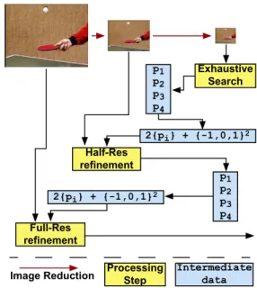
3.3 Multiresolution and Multiprediction Algorithm We now consider 640 per 480 images and blocks of length 16. We only use the luminance, so it is preferable to reduce the image to a single channel as soon as possible. Our al-gorithm uses several images at different resolutions. Each image has to be filtered and downsampled by a factor of two in each dimension, leading to a 320 per 240 half resolution image. Applying this again leads to a 160 per 120 quarter resolution image. In order to reduce processing time, it is convenient to apply a separable filter.
The first step is to compute the function c for any block and any possible vector in the range [ 16,16] ⇥ [ 8,8] at the quarter-resolution, leading to a motion cost table. Then, among all these results, we select the four smallest per
block, keeping four predictors (~pi)i=0..3. Considering 4 per 4
blocks, this may be seen as an exhaustive search for a list of the 4 best vectors.
All these predictors are multiplied by two before using them at the half-resolution. Then, for each block, whose size is now 8 per 8, we consider up to thirty six vectors: four predictors plus all their neighbours, i.e. the set of vectors
{2 ⇥~pi+ { 1,0,1}2}, whose cardinalty may be below 36 in
the case of two adjacent predictors. Among these 36 possi-bilites, we still take the four best, leading to four new
pre-dictors (~p0
i)i=0..3. Moving back to the full-resolution follows
exactly the same principle, considering a new set of vectors
{2 ⇥ ~p0i+ { 1,0,1}2}, and we only keep the best result at
this step. This processing is summarized in figure 2.
Exhaustive Search Half-Res refinement Full-Res refinement p1 p2 p3 p4 2{pi} + {-1,0,1}2 p1 p2 p3 p4 Processing Step Intermediate data Image Reduction 2{pi} + {-1,0,1}2
Figure 2: Multiresolution Multiprediction Algorithm This provides us with a good algorithmic quality for a still reasonable computation cost and the algorithm is almost reg-ular enough to fit in the GPU datastream model.
4. IMPLEMENTATION SPECIFICITIES The first particularity of a GPU implementation of a complex algorithm is that it has to be cut into several steps, each step being seen as a computational kernel applied to a large set of data. This computational kernel may also be seen as a loop body, the loop being controlled by the API and through the rasterization of all fragments. All kernels have to perform a limited amount of computations and memory accesses. On the implementation side, image reduction may be per-formed automatically by the GPU. In order to control the fil-ter and to be sure of the result, we implemented these steps ourselves. The whole reduction process is done in four one-dimension reductions, one horizontal and one vertical lead-ing to the half-resolution, and again to the quarter-resolution. Moving to the quarter-resolution, all values of the c function are computed at once, generating a set of 673.000 distances - one per couple block / vector, with 40 per 30 blocks and 33 per 17 vectors. Then, another set of fragment programs gathers in several steps all these results in order to find the minimum value per block among all possible vectors. This leads to a set of 40 per 30 values: all the best vectors. These results are read and the corresponding entries in the distance table overwritten by the vertex processors, setting them to the maximum. This way, gathering again the results leads to the second best vectors. This is performed twice again in order to get four vectors. It is interesting to note that get-ting all vectors may have been implemented in a single pass.
But this would have reduced flexibility and the performance gain would not have been that obvious: each gathering step would have been done between eight values, i.e. gathering the results of two executions at once, then sorting these eight values would have been necessary. Sorting is an expensive task on the GPU, mostly due to the fact that the fragment processors are almost SIMD. This implies that in if-cases, both branches are executed by all processors. This penalty is to be added to the expensive overhead of such structures. Then, having all these predictors, we may move back to the half-resolution. This is first performed by a fragment pro-gram that fetches predictors, computes the memory location of the translated block, fetches both blocks and computes partial sums of our c function. We have to stop at partial sums to prevent a too large amount of memory accesses at once. Another fragment program gathers all these results and pro-vides a half-resolution c table. Then, as previously, another set of fragment programs is used to gather and compare all these results. This leads to the best vector per block. As pre-viously again, the Vertex Processors disable corresponding entries and the processing is performed several times again,
leading to the (~p0
i)ifamily of predictors.
Returning to the full resolution lies on the same principles, except that we stop with the first result instead of looking for four. Another difference is the fact that the gathering of par-tial sums has to be performed in two steps as the number of samples to be fetched increases. During the whole process-ing, vector location has been encoded recursively. In fact, we encoded recursively the information of where any selected value comes from during the gathering, what allows to build back the whole vector. So this contains all information on selected vectors: our result may be sent back to the CPU.
5. APPLICATIONS AND RESULTS
On its own, our Block-Matching runs at 17.5 fps on a 6800GT board, compared to 1.61 fps on a dual 3 Ghz Pentium-IV. Using only one predictor when moving from the half- to the full-resolution yields 27.4 fps. Whatever the quantity of predictors, the acceleration factor is always more than ten. A drawback shall be noticed in the setup time for the first couple of images; this represents a few seconds. As a proof of concept, we decided to use this motion-estimator in a video encoder, using thus the GPU as a copro-cessor dedicated to that specific task whereas the CPU had to handle all other MPEG processings.
Starting from the Dali library[11] and using their sim-ple MPEG-1 encoder examsim-ple, we replaced the motion-estimation section, adding the same software control that al-lows thresholding on the null motion or intra-coding accord-ingly to the result quality. The Motion-Estimation used by Dali is a fast logarithmic search used only after checking that null-motion is not sufficent. We have also separated the API calls in a separate thread: this lets some MPEG-processing be done while waiting for the GPU to finish and for the API to unlock the execution of its thread.
Comparing with the original encoder, the speed has been im-proved by 65%, increasing from 6 to 10 frames per second on our hardware. On the first experiments, we had neither in-crease in quality nor reduction in mpeg filesize. This was due to the poor quality of the sequences we worked on, which were mpeg-2 classical test sequences. Working on a clean succession of images and specifying a constant
signal-to-noise ratio, we got a 10-15% reduction in file sizes, thereby validating the algorithmical quality of our method.
6. CONCLUSION
In this contribution, we have shown that the processing power of the GPU can be used to off-load the CPU. Graphics Hardware can be used efficiently as a Digital Signal Copro-cessor, thanks to their massively parallel architecture. As the main processor still has to perform control, the GPU can be used as a coprocessor only.
To prove this concept, we successfully implemented a Block-Matching motion estimator whose speed has been increased by a factor of more than 10 when compared to its CPU imple-mentation. Then, we tested this for MPEG Encoding. It lead to significant improvements in several fields such as speed, processor load and algorithmic quality.
Future work includes a more flexible implementation with for instance the possibility to parametrize block sizes, image sizes, half- and full-resolution refinement sets of
vectors... Another step will be the integration in the
GPUCV framework. As a part of the VisionGPU
Project (http://picolibre.int-evry.fr/projects/gpucv/), it has been funded by the french GET (http://www.get-telecom.fr/), a network of Engineering Schools.
REFERENCES
[1] V. Bhaskaran and K. Konstantinidies, Image and Video Compression Standards. Kluwer Academic Publishers, 1997.
[2] M. I. Sezan and R. L. Lagendijk, Motion Analysis and Image Sequence Processing. Kluwer Academic Publish-ers, 1993.
[3] C. Tziritas and C. Labit, Motion Analysis for Image Se-quence Coding. Elsevier, 1994.
[4] K. R. Rao and J. J. Hwang, Techniques & Standards for Image, Video & Audio Coding. Prentice Hall PTR, 1996. [5] GPUGems - Programming Techniques, Tips, and Tricks
for Real-Time Graphics. nVidia, Inc. 2004.
[6] GPUGems 2 - Programming Techniques for High-Performance Graphics and General-Purpose Computa-tion. nVidia, Inc. 2005.
[7] J. Montrym and H. Moreton, “The geForce 6800”. In Mi-cro, IEEE, vol. 25 iss. 2, pp. 41–51, 2005.
[8] T. Dokken, T. Hagen and J. M. Hjelmervik, “The GPU as a high performance computational resource,” in Pro-ceedings of the 21st Spring Conference on Computer Graphics, ACM Press.
[9] N. Goodnight, R. Wand and G. Humphreys, “Compu-tation on Programmable Graphics Hardware”. In Com-puter Graphics and Applications, IEEE, vol. 25 iss. 5, 2005.
[10] J. D. Owens, D. Luebke, N. Govindaraju, M. Harris, J. Kuger, A. E. Lefohn, and T. J. Purcell, “A survey of General-Purpose Computation on Graphics Hardware”. In EUROGRAPHICS 2005, State of the Art reports, pp. 21–51, 2005.
[11] W.T. Ooi, B. Smith, S. Mukhopadhyay, H.H. Chan, S. Weiss, and M. Chiu, The Dali Multimedia Software Li-brary. December, 1998.