HAL Id: hal-01056397
https://hal.archives-ouvertes.fr/hal-01056397
Submitted on 20 Aug 2014
HAL is a multi-disciplinary open access
archive for the deposit and dissemination of
sci-entific research documents, whether they are
pub-lished or not. The documents may come from
teaching and research institutions in France or
abroad, or from public or private research centers.
L’archive ouverte pluridisciplinaire HAL, est
destinée au dépôt et à la diffusion de documents
scientifiques de niveau recherche, publiés ou non,
émanant des établissements d’enseignement et de
recherche français ou étrangers, des laboratoires
publics ou privés.
Motion Trajectories on Riemannian Manifold
Maxime Devanne, Hazem Wannous, Stefano Berretti, Pietro Pala, Mohamed
Daoudi, Alberto del Bimbo
To cite this version:
Maxime Devanne, Hazem Wannous, Stefano Berretti, Pietro Pala, Mohamed Daoudi, et al.. 3D
Human Action Recognition by Shape Analysis of Motion Trajectories on Riemannian Manifold. IEEE
Transactions on Cybernetics, IEEE, 2015, 45 (7), pp.1340-1352. �hal-01056397�
3D Human Action Recognition by Shape Analysis
of Motion Trajectories on Riemannian Manifold
Maxime Devanne, Hazem Wannous, Stefano Berretti, Pietro Pala, Mohamed Daoudi, and Alberto Del Bimbo
Abstract—Recognizing human actions in 3D video sequences is an important open problem that is currently at the heart of many research domains including surveillance, natural interfaces and rehabilitation. However, the design and development of models for action recognition that are both accurate and efficient is a challenging task due to the variability of the human pose, clothing and appearance. In this paper, we propose a new framework to extract a compact representation of a human action captured through a depth sensor, and enable accurate action recognition. The proposed solution develops on fitting a human skeleton model to acquired data so as to represent the 3D coordinates of the joints and their change over time as a trajectory in a suitable action space. Thanks to such a 3D joint-based framework, the proposed solution is capable to capture both the shape and the dynamics of the human body simultaneously. The action recognition problem is then formulated as the problem of computing the similarity between the shape of trajectories in a Riemannian manifold. Classification using kNN is finally performed on this manifold taking advantage of Riemannian geometry in the open curve shape space. Experiments are carried out on four representative benchmarks to demonstrate the potential of the proposed solution in terms of accuracy/latency for a low-latency action recognition. Comparative results with state-of-the-art methods are reported.
Index Terms—3D human action, activity recognition, temporal modeling, Riemannian shape space.
I. INTRODUCTION
I
MAGING technologies have recently shown a rapidad-vancement with the introduction of consumer depth cam-eras (RGB-D) with real-time capabilities, like Microsoft Kinect [1] or Asus Xtion PRO LIVE [2]. These new ac-quisition devices have stimulated the development of various promising applications, including human pose reconstruction and estimation [3], scene flow estimation [4], hand gesture recognition [5], and face super-resolution [6]. A recent review of kinect-based computer vision applications can be found in [7]. The encouraging results shown in these works take advantage of the combination of RGB and depth data enabling simplified foreground/background segmentation and increased robustness to changes of lighting conditions. As a result, several software libraries make it possible to fit RGB and depth M. Devanne is with the University Lille 1 (Telecom Lille), Laboratoire d’Informatique Fondamentale de Lille (LIFL - UMR CNRS 8022), Lille, France and with the Media Integration and Communication Center, University of Florence, Florence, Italy (e-mail: maxime.devanne@telecom-lille.fr).
H. Wannous is with the University Lille 1, Laboratoire d’Informatique Fondamentale de Lille (LIFL - UMR CNRS 8022), Lille, France (e-mail: hazem.wannous@telecom-lille.fr).
M. Daoudi is with Telecom Lille/Institut Mines-Telecom, Laboratoire d’Informatique Fondamentale de Lille (LIFL - UMR CNRS 8022), Lille, France (e-mail: mohamed.daoudi@telecom-lille.fr).
S. Berretti, P. Pala and A. Del Bimbo are with the Media Integration and Communication Center, University of Florence, Florence, Italy (e-mail: stefano.berretti@unifi.it, pietro.pala@unifi.it, delbimbo@dsi.unifi.it).
models to the data, thus supporting detection and tracking of skeleton models of human bodies in real time. However, solutions which aim to understand the observed human actions by interpreting the dynamics of these representations are still quite limited. What further complicates this task is that action recognition should be invariant to geometric transformations, such as translation, rotation and global scaling of the scene. Additional challenges come from noisy or missing data, and variability of poses within the same action and across different actions. In this paper, we address the problem of modeling and analyzing human motion from skeleton sequences captured by depth cameras. Particularly, our work focuses on building a robust framework, which recasts the action recognition problem as a statistical analysis on the shape space manifold of open curves. In such a framework, not only the geometric ap-pearance of the human body is encoded, but also the dynamic information of the human motion. Additionally, we evaluate the latency performance of our approach by determining the number of frames that are necessary to permit a reliable recognition of the action.
A. Previous Work
In recent years, recognition of human actions from the analysis of data provided by RGB-D cameras has attracted the interest of several research groups. The approaches proposed so far can be grouped into three main categories, according to the way they use the depth channel: skeleton-based, depth map-based and hybrid approaches. Skeleton based approaches, estimate the position of a set of joints of a human skeleton fitted to depth data. Then they model the pose of the human body in subsequent frames of the sequence using the position and the relations between joints. Depth map based approaches extract volumetric and temporal features directly from the overall set of points of the depth maps in the sequence. Hybrid approaches combine information extracted from both the joints of the skeleton and the depth maps. In addition to these approaches, there are also some multi-modal methods that exploit both depth and photometric information to improve results [8]. Following this categorization, existing methods for human action recognition using depth information are shortly reviewed below.
Skeleton based approaches have become popular thanks to the work of Shotton et al. [3]. This describes a real-time method to accurately predict the 3D positions of body joints in individual depth maps, without using any temporal information. Results report the prediction accuracy for 16 joints, although the Kinect tracking system developed on top of this approach is capable of estimating the 3D positions of 20
joints of the human skeleton. In [9], an approach is described to support action recognition based on the histograms of the position of 12 joints provided by the Kinect. The histograms are projected using LDA and clustered into k posture visual words, representing the prototypical poses of the actions. The temporal evolution of these visual words is modeled by discrete Hidden Markov Models. In [10], human action recognition is obtained by extracting three features for each joint, based on pair-wise differences of joint positions: in the current frame; between the current frame and the previous frame; and between the current frame and the initial frame of the sequence. This latter is assumed to correspond to the neutral posture at the beginning of the action. Since the number of these differences results in a high dimensional feature vector, PCA is used to reduce redundancy and noise, and to obtain a compact EigenJoints representation of each frame. Finally, a na¨ıve-Bayes nearest-neighbor classifier is used for multi-class action classification. Recent works address more complex challenges in on-line action recognition systems, where a trade-off between accuracy and latency becomes an important goal. For example, Ellis et al. [11] target this trade-off by adopting a Latency Aware Learning method for reducing latency when recognizing human actions. A logistic regression-based classifier is trained on 3D joint position sequences to search a single canonical posture for recognition. Methods based on depth maps rely on the extraction of meaningful descriptors from the entire set of points of depth images. Different methods have been proposed to model the dynamics of the actions. The approach in [12] employs 3D human silhouettes to describe salient postures and uses an action graph to model the dynamics of the actions. In [13], the action dynamics is described using Depth Motion Maps, which highlight areas where some motion takes place. Other methods, such as Spatio-Temporal Occupancy Pattern [14], Random Occupancy Pattern [15] and Depth Cuboid Similarity Feature [16], propose to work on the 4D space divided into spatio-temporal boxes to extract features representing the depth appearance in each box. Finally, in [17] a method is proposed to quantize the 4D space using vertices of a polychoron and then model the distribution of the normal vectors for each cell. Depth information can also be used in combination with color images as in [18].
Hybrid solutions use strengths of both skeleton and depth descriptors to model the action sequence. For example, in [19] a Local Occupancy Pattern around each 3D joint is proposed. In [20], actions are characterized using pairwise affinity mea-sures between joint angle features and histogram of oriented gradients computed on depth maps.
These RGB-D based approaches also benefit from the large number of works published in the last two decades on human activity recognition in 2D video sequences (see for example the recent surveys in [21], [22], [23], [24]). Besides methods in Euclidean spaces [25], [26], [27], some emerging and interesting techniques reformulate computer vision problems, like action recognition, over non-Euclidean spaces. Among these, Riemannian manifolds have recently received increased attention. In [28] human silhouettes extracted from video
images are used to represent the pose. Silhouettes are then represented as points in the shape space manifold. In this way, they can be matched using a Dynamic Time Warping, a state-of-the-art algorithm for sequence comparison. In [29] several experiments on gesture recognition and person re-identification are conducted, comparing Riemannian manifolds with several state-of-the-art approaches. Results obtained in these works indicate considerable improvements in discrimination accu-racy. In [30], a Grassmann manifold is used to classify human actions. With this representation, a video sequence is expressed as a third-order data tensor of raw pixels extracted from action images. One video sequence is mapped onto one point on the manifold. Distances between points are computed on the manifold and used for action classification based on nearest neighbor search.
B. Overview of Our Approach
A human action is naturally characterized by the evolution of the pose of the human body over time. Skeleton data containing the 3D positions of different parts of the body provide an accurate representation of the pose. These skeleton features are easy to extract and track from depth maps, and they also provide local information about the human body. This makes it possible to analyze only some parts of the human body instead of the global pose. Even if accurate 3D joint positions are available, the action recognition task is still difficult due to significant spatial and temporal variations in the way of performing an action.
These challenges motivated the study an original approach to recognize human actions based on the evolution of the position of the skeleton joints detected on a sequence of depth images. To this end, the full skeleton is modeled as a multi-dimensional vector obtained by concatenating the three-dimensional coordinates of its joints. Then, the trajectory described by this vector in the multi-dimensional space is regarded as a signature of the temporal dynamics of the move-ments of all the joints. These trajectories are then interpreted in a Riemannian manifold, so as to model and compare their shapes using elastic registration and matching in the shape space. In so doing, we recast the action recognition problem as a statistical analysis on the shape space manifold. Furthermore, by using an elastic metric to compare the similarity between trajectories, robustness of action recognition to the execution speed of the action is improved. Figure 1 summarizes the proposed approach. The main considerations that motivated our solution are: (1) The fact that many feature descriptors typically adopted in computer vision applications lie on curved spaces due to the geometric nature of the problems; (2) The shape and dynamic cues are very important for modeling human activity, and their effectiveness have been demonstrated in several state-of-the-art works [30], [31], [32], [33]; (3) Using such manifold offers a wide variety of statistical and modeling tools that can be used to improve the accuracy of gesture and action recognition.
The main contributions of the proposed approach are:
• An original translation and rotation invariant
Fig. 1: Overview of our approach: First, skeleton sequences are represented as trajectories in a n-dimensional space; These trajectories are then interpreted in a Riemannian manifold (shape space); Recognition is finally performed using kNN classification on this manifold.
dimensional space. By concatenating the 3D coordinates of skeleton joints, data representation encodes the shape of the human posture at each frame. By modeling the se-quence of frame features along the action as a trajectory, we capture the dynamics of human motion;
• An elastic shape analysis of such trajectories that extends
the shape analysis of curves [34] to action trajectories, thus improving robustness of action recognition to the execution speed of actions.
The rest of the paper is organized as follows: Sect. II de-scribes the proposed spatio-temporal representation of actions as trajectories; Sect. III discusses the Riemannian framework used for the analysis and comparison of shape trajectories; In Sect. IV, we present some statistical tools applicable on a Riemannian manifold and introduce the supervised learning algorithm performed on points of this manifold; Sect. V describes the experimental settings, the dataset used and also reports results in terms of accuracy and latency of action recognition in comparison with state of the art solutions; Finally, in Sect. VI conclusions are drawn and future research directions discussed.
II. SPATIO-TEMPORALREPRESENTATION OFACTIONS AS
TRAJECTORIES IN THEACTIONSPACE
Using RGB-D cameras, such as the Microsoft Kinect, a 3D humanoid skeleton can be extracted from depth images in real-time by following the approach of Shotton et al. [3]. This skeleton contains the 3D position of a certain number of joints representing different parts of the human body. The number of estimated joints depends on the SDK used in combination with the device. Skeletons extracted with the Microsoft Kinect SDK contain 20 joints, while 15 joints are estimated with the PrimeSense NiTE. For each frame t of a sequence, the real-world 3D position of each joint i of the skeleton is represented by three coordinates expressed in the camera reference system pi(t) = (xi(t), yi(t), zi(t)). Let Nj be the number of joints
the skeleton is composed of, the posture of the skeleton at
frame t is represented by a 3Nj dimensional tuple:
v(t) = [x1(t) y1(t) z1(t) . . . xNj(t) yNj(t) zNj(t)]
T . (1)
For an action sequence composed of Nf frames, Nf feature
vectors are extracted and arranged in columns to build a feature matrix M describing the whole sequence:
M = v(1) v(2) . . . v(Nf) . (2)
This feature matrix represents the evolution of the skeleton pose over time. Each column vector v is regarded as a sample
of a continuous trajectory in R3Nj representing the action in a
3Nj dimensional space called action space. The size of such
feature matrix is 3Nj⇥ Nf.
To reduce the effect of noise that may affect the coordi-nates of skeleton joints, a smoothing filter is applied to each sequence. This filter weights the coordinates of each joint with the coordinates of the same joint in the neighboring frames. In particular, the amount of smoothing is controlled
by a parameter that defines the size Ws = 1 + 2⇥ of a
temporal window centered at the current frame. For each joint
i = 1, . . . , Nj at frame t = 1 + , . . . , Nf the new x
coordinate is: xi(t) = 1 Ws t+ X ⌧ =t xi(⌧ ) . (3)
The same applies to y and z. The value of is selected
by performing experiments on a set of training sequences.
The best accuracy is obtained for = 1, corresponding to
a window size of 3 frames.
A. Invariance to Geometric Transformations of the Subject A key feature of action recognition systems is the invariance to the translation and rotation of the subject in the scene: Two instances of the same action differing only for the position and orientation of the person with respect to the scanning device should be recognized as belonging to the same action class. This goal can be achieved either by adopting a translation and rotation invariant representation of the action sequence or providing a suitable distance measure that copes with translation and rotation variations. We adopt the first approach by normalizing the position and the orientation of the subject in the scene before the extraction of the joint coordinates. For this purpose, we first define the spine joint of the initial skeleton as the center of the skeleton (root joint). Then, a new base B is defined with origin in the root joint: it includes the left-hip joint vector !hl, the right-hip joint vector !hr, and
their cross product !nB = !hl ⇥!hr. This new base is then
translated and rotated, so as to be aligned with a reference
base B0 computed from a reference skeleton (selected as the
neutral pose of the sequence). The calculation of the optimal
rotation between the two bases B and B0 is performed using
Singular Value Decomposition (SVD). For each sequence, once the translation and the rotation of the first skeleton is computed with respect to the reference skeleton, we apply the same transformations to all other skeletons of the sequence. This makes the representation invariant to the position and orientation of the subject in the scene. Figure 2a shows an
example of two different skeletons to be aligned. The bases B1
and B2computed for the two skeletons are shown in Fig. 2b,
where the rotation required to align B2 to B1is also reported.
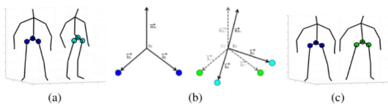
(a) (b) (c) Fig. 2: Invariance to geometric transformations: (a) Two skeletons with different orientations. The skeleton on the left is the reference one. The skeleton on the right is the first skeleton of the sequence that should be aligned to the
reference skeleton; (b) Bases B0 and B are built from the
two corresponding hip vectors and their cross product. The
base B0 corresponds to B aligned with respect to B
0; (c) The
resulting skeleton (right) is now aligned with respect to the first one (left). The transformations computed between these two bases are applied to all skeletons of the sequence. B. Representation of Body Parts
In addition to enable the representation of the action using the whole body, the proposed solution also supports the representation of individual body parts, such as the legs and the arms. There are several motivations for focusing on parts of the body. First of all, many actions involve motion of just some parts of the body. For example, when subjects answer a phone call, they only use one of their arms. In this case, analyzing the dynamics of the arm rather than the dynamics of the entire body is expected to be less sensitive to the noise originated by the involuntary motion of the parts of the body not directly involved in the action. Furthermore, during the actions some parts of the body can be out of the camera field of view or occluded by objects or other parts of the body. This can make the estimation of the coordinates of some joints inaccurate, compromizing the accuracy of action recognition. Finally, due the symmetry of the body along the vertical axis, one same action can be performed using one part of the body or another. With reference to the action “answer phone call”, the subject can use his left arm or right arm. By analyzing the whole body we can not detect such variations. Differently, using body parts separately, simplifies the detection of this kind of symmetrical actions. To analyze each part of the body separately, we represent a skeleton sequence by four feature sets corresponding to the body parts. Each body part is associated with a feature set that is composed of the 3D normalized position of the joints that are included in that part
of the body. Let Njp be the number of joints of a body part,
the skeleton sequence is now represented by four trajectories
in 3 ⇥ Njp dimensions instead of one trajectory in 3 ⇥ Nj
dimensions. The actual number of joints per body part can change from a dataset to another according to the SDK used
for estimating the body skeleton. In all the cases, Njp < Nj
and the body parts are disjoint (i.e., they do not share any joint).
III. SHAPEANALYSIS OFTRAJECTORIES
An action is a sequence of poses and can be regarded as the result of sampling a continuous curve trajectory in the
3Nj-dimensional action space. The trajectory is defined by
the motion over time of the feature point encoding the 3D coordinates of all the joints of the skeleton (or by all the feature points coding the body parts separately). According to this, two instances of the same action are associated with two curves with similar shape in the action space. Hence, action recognition can be regarded and formulated as a shape matching task. Figure 3 provides a simplified example of action matching by shape comparison. The plot displays five curves corresponding to the coordinates of the left hand joint in five different actions. Three curves correspond to three instances of the action drawing circle. The remaining two curves correspond to the actions side boxing and side kick. This simplified case, in which each trajectory encodes the coordinates of just one joint, makes it clear that similar actions yield trajectories with similar shapes in the action space.
Fig. 3: Curves representing the coordinates of the left arm joint for five actions: From left to right, side kick, side boxing, and draw circle (three different instances). Points displayed in bold represent the sample frames along the curves.
Figure 3 also highlights some critical aspects of representing actions by trajectories. Assuming the actions are sampled at the same frame rate, performing the same action at two different speeds yields two curves with a different number of samples. This is the case of the red and blue curves in Fig. 3, where samples are highlighted by bold points along the curves. Furthermore, since the first and the last poses of an action are not known in advance and may differ even for two instances of the same action, the measure of shape similarity should not be biased by the position of the first and last points of the trajectory. In the following we present a framework to represent the shape of the trajectories, and compare them using the principles of elastic shape matching.
A. Representation of Trajectories
Let a trajectory in the action space be represented as a
function : I ! Rn, being I = [0,1] the function domain.
We restrict the domain of interest to the functions that
are differentiable and whose first derivative is in L2(I, Rn).
L2(I, Rn) is the vector space of all functions f : I ! Rn
satisfyingRIkf(x)k2dx <1. To analyze the shape of , we
consider its square-root velocity function (SRVF) q : I ! Rn,
defined as:
q(t)=. q˙(t)
k ˙(t)k
being k.k the L2norm. The quantity kq(t)k is the square-root
of the instantaneous speed, and the ratio q(t)
kq(t)k is the
instan-taneous direction along the trajectory. All trajectories are
scaled so as to be of length 1. This makes the representation invariant to the length of the trajectory (the number of frames of the action sequence). The SRVF was formerly introduced in [34] to enable shape analysis. As described in [34], such
representation captures the shape of a curve and presents
some advantages. First, it uses a single function to represent the curve. Then, as described later, the computation of the
elastic distance between two curves is reduced to a simple L2
norm, which simplifies the implementation and the analysis. Finally, re-parametrization of the curves acts as an isometry. The SRVF has been successfully used for 3D face recognition in [35] and for human body matching and retrieval in [36]. In our approach we propose to extend this metric to the analysis of spatio-temporal trajectories.
B. Pre-shape Space of Trajectories We define the set of curves:
C = {q : I ! Rn
| kqk = 1} ⇢ L2(I, Rn) , (5)
where k.k represents the L2 norm. With the L2 norm on its
tangent space, C becomes a Riemannian manifold called pre-shape space. Each element of C represents a trajectory in
Rn. As the elements of this manifold have unit L2 norm,
C is a unit-hypersphere representing the pre-shape space of trajectories invariant to uniform scaling. Its tangent space at a point q is given by:
Tq(C) = {v 2 L2(I, Rn)| hv, qi = 0} . (6)
Here, hv, qi denotes the inner product in L2(I, Rn).
Geodesics on spheres are great circles, thus the geodesic
path between two elements q1 and q2 on C is given by the
great circle ↵:
↵(⌧ ) = 1
sin(✓)(sin((1 ⌧ )✓)q1+ sin(✓⌧ )q2) , (7)
where ✓ is the distance between q1 and q2 given by:
✓ = dc(q1, q2) = cos 1(hq1, q2i) . (8)
This equation measures the geodesic distance between two
trajectories q1 and q2 represented in the manifold C. In
particular, ⌧ 2 [0, 1] in Eq. (7) allows us to parameterize the movement along the geodesic path ↵. ⌧ = 0 and ⌧ = 1,
correspond, respectively, to the extreme point q1 and q2 on
the geodesic path. For intermediate values of ⌧, an internal
point between q1 and q2on the geodesic path is considered.
C. Elastic Metric in the Shape Space
As mentioned above, we need to compare the shape of the trajectories independently of their elasticity. This requires in-variance to re-parameterization of the curves. Let us define the parameterization group , which is the set of all orientation-preserving diffeomorphisms of I to itself. The elements 2
are the re-parameterization functions. For a curve : I ! Rn,
is a re-parameterization of . As shown in [37], the
SRVF of is given by p˙ (t)(q )(t). We define the
equivalent class of q as:
[q] ={p˙ (t)(q )(t)| 2 } . (9)
The set of such equivalence classes is called the shape space of elastic curves, noted S = {[q] | q 2 C}. In this framework, an equivalent class [q] is associated to a shape. Accordingly,
comparison of the shapes of two trajectories q1 and q2, is
performed by the comparison of the equivalent classes [q1]and
[q2]. Computation of the geodesic paths and geodesic lengths,
requires to solve the optimization problem for finding the
opti-mal re-parameterization that best registers the element q2with
respect to q1. The optimal re-parameterization ⇤ is the one
that minimizes the cost function H( ) = dc(q1,p˙ (q2 )).
Thus, the optimization problem is defined as:
⇤= arg min
2 dc(q1,
p
˙ (q2 )) . (10)
In practice, dynamic programming is used for optimal re-parameterization over .
Let q⇤
2 =
p
˙⇤(q2 ⇤)be the optimal element associated
with the optimal re-parameterization ⇤ of the second curve
q2, the geodesic length between [q1]and [q2]in the shape space
S is ds([q1], [q2]) = dc(q1, q2⇤)and the geodesic path is given
by:
↵(⌧ ) = 1
sin(✓)(sin((1 ⌧ )✓)q1+ sin(✓⌧ )q
⇤
2) , (11)
where ✓ = ds([q1], [q2]). This distance is used to compare the
shape of the trajectories in a way that is robust to their elastic deformation.
IV. ACTION RECOGNITION ON THE MANIFOLD
The proposed action recognition approach is based on the K-Nearest Neighbors (kNN) algorithm applied both to full-body and separate full-body parts.
A. kNN classifier using an elastic metric
Let {(Xi,yi)}, i = 1, . . . , N, be the training set with
respect to the class labels, where Xi belongs to a
Rieman-nian manifold S, and yi is the class label taking values in
{1, . . . , Nc}, with Nc the number of classes. The objective is
to find a function F (X) : S 7 ! {1, . . . , Nc} for clustering
data lying in different submanifolds of a Riemannian space, based on the training set of labeled items of the data. To this end, we propose a kNN classifier on the Riemannian manifold, learned by the points on the open curve shape space representing trajectories. Such learning method exploits geo-metric properties of the open curve shape space, particularly its Riemannian metric. This relies on the computation of the (geodesic) distances to the nearest neighbors of each data point of the training set.
The action recognition problem is reduced to nearest neigh-bor classifier in the Riemannian space. More precisely, given
a set of training trajectories Xi : i = 1, . . . , N, they are
map trajectories on the shape space manifold (see Fig. 1).
Then, any new trajectory Xn is represented by its SRVF qn.
Finally, a geodesic-based classifier is used to find the
K-closest trajectories to qn using the elastic metric given by
Eq. (8).
B. Statistics of the Trajectories
An important advantage of using such Riemannian approach is that it provides tools for the computation of statistics of the trajectories. For example, we can use the notion of Karcher mean [38] to compute an average trajectory from several trajectories. The average trajectory among a set of different trajectories can be computed to represent the intermediate one, or between similar trajectories obtained from several subjects to represent a template, which can be viewed as a good representative of a set of trajectories.
To classify an action trajectory, represented as a point on the manifold, we need to compute the total warping geodesic distances to all points from training data. For a large number of training data this can be associated to a high computational cost. This can be reduced by using the notion of “mean” of class action, and computing the mean of a set of points on the manifold. As a result, for each action class we obtain an average trajectory, which is representative of all the actions within the class. According to this, the mean can be used to perform action classification by comparing the new action with all the cluster means using the elastic metric defined in Eq. (8). For a given set of training trajectories q1, . . . , qn on the shape
space, their Karcher mean can be defined as: µ = arg min
n
X
i=1
ds([q], [qi])2. (12)
As an example, Fig. 4a shows the Karcher mean computa-tion for five training trajectories (q1. . . q5). In the initial step,
q1 is selected as the mean. In an iterative process, the mean
is updated according to elastic metric computation between all q. After convergence, the average trajectory is given by
qm. Fig. 4b shows skeleton representation of the first two
trajectories and the resulting average trajectory in the action space. As trajectories are built from joint coordinates, we can easily obtain the entire skeleton sequence corresponding to a trajectory. Figure 4b shows four skeletons for each sequence. By computing such average trajectories for each action class, we implicitly assume that there is only one way to perform each action. Unfortunately, this is not the case. In fact, two different subjects can perform the same action in two different ways. This variability in performing actions between different subjects can affect the computation of average trajectories and the resulting templates may not be good representatives of the action classes. For this reason, we compute average trajectories for each subject, separately. Instead of having only one representative trajectory per action, we obtain one template per subject per action. In this way, we keep separately each different way of performing the action and the resulted average trajectories are not any more affected by such possible variations. As a drawback, with this solution the number of template trajectories in the training
(a) (b)
Fig. 4: Computation of the Karcher mean between five action trajectories: (a) Representation of the trajectories in the shape space. Applying the Karcher mean algorithm, the mean is first
selected as q1and then updated until convergence. Finally, the
mean trajectory is represented by qm; (b) Skeleton
represen-tation of corresponding trajectories in the action space. The
two top sequences correspond to points q1and q2in the shape
space, while the bottom sequence corresponds to the Karcher
mean qm computed among the five training trajectories.
set increases. Let Nc be the number of classes and NStr the
number of subjects in the training set, the number of training
trajectories is Nc⇥ NStr. However, as subjects perform the
same action several times, the number of training trajectories is still lower than using all trajectories.
C. Body parts-based classification
In the classification step, we compute distances between corresponding parts of the training sequence and the new sequence. As a result, we obtain four distances, one for each body part. The mean distance is computed to obtain a global distance representing the similarity between the training sequence and the new sequence. We keep only the k smallest global distances and corresponding labels to take the decision and associate the most frequent label to the new sequence. Note that in the case where some labels are equally frequent, we apply a weighted decision based on the ranking of the distances. In that particular case, the selected label corresponds to the smallest distance. However, one main motivation for considering the body parts separately is to analyze the moving parts only. To do this, we compute the total motion of each part over the sequence. We cumulate the Euclidian distances between corresponding joints in two consecutive frames for all the frames of the sequence. The total motion of a body part is the cumulated motion of the joints forming this part. We compute this total motion on the re-sampled sequences, so that it is not necessary to normalize it. Let jk : k = 1, . . . , N
jp,
be a joint of the body part, and Nf be the frame number of
the sequence, then the total motion m of a body part for this sequence is given by:
m = Njp X k=1 Nf 1 X i=1 dEuc(jik, ji+1k ) , (13)
where dEuc(j1, j2)is the Euclidian distance between the 3D
part (i.e., this number can change from a dataset to another according to the SDK used for the skeleton estimation).
Once the total motion for each part of the body is computed,
we define a threshold m0 to separate moving and still parts.
We assume that if the total motion of a body part is below this threshold, the part is considered to be motionless during the action. In the classification, we consider a part of the body only if it is moving either in the training sequence or the probe sequence (this is the sequence representing the action to be classified). If one part of the body is motionless in both actions, this part is ignored and does not concur to compute the distance between the two actions. For instance, if two actions are performed only using the two arms, the global distance between these two actions is equal to the mean of the distances corresponding to the arms only. We empirically
select the threshold m0 that best separates moving and still
parts with respect to a labeled training set of ground truth sequences. To do that, we manually labeled a training set of sample sequences by assigning a motion binary value to each body part. The motion binary value is set to 1 if the body part is moving and set to 0 otherwise. We then compute the total motion m of each body part of the training sequences and give a motion decision according to a varying threshold. We finally select the threshold that yields the decision closest to the ground truth. In the experiments, we notice that defining two different thresholds for the upper parts and lower parts slightly improves the accuracy in some cases.
V. EXPERIMENTALEVALUATION
The proposed action recognition approach is evaluated in comparison to state-of-the-art methods using three public benchmark datasets. In addition, we measure the capability of our approach to reduce the latency of recognition by evaluating the trade-off between accuracy and latency over a varying number of actions.
A. Datasets
The three benchmark datasets that we use to evaluate the accuracy of action recognition differ in the characteristics and difficulties of the included sequences. This allows an in depth investigation of the strengths and weaknesses of our solution. For each dataset, we compare our approach to state-of-the-art methods. A fourth dataset (UCF-kinect) is used for the latency analysis.
a) MSR Action 3D: This public dataset was collected
at Microsoft research [12] and represents a commonly used benchmark. It includes 20 actions performed by 10 persons facing the camera. Each action is performed 2 or 3 times. In total, 567 sequences are available. The different actions are high arm wave, horizontal arm wave, hammer, hand catch, forward punch, high throw, draw X, draw tick, draw circle, hand clap, two hand wave, side-boxing, bend, forward kick, side kick, jogging, tennis swing, tennis serve, golf swing, pick up & throw. These game-oriented actions cover different varia-tions of the motion of arms, legs, torso and their combinavaria-tions. Each subject is facing the camera and positioned in the center of the scene. Subjects were also advised to use their right
arm or leg when actions are performed with a single arm or leg. All the actions are performed without any interaction with objects. Two main challenges are identified: the high similarity between different groupg of actions and the changes of the execution speed of actions. For each sequence, the dataset provides depth, color and skeleton information. In our case, we only use the skeleton data. As reported in [19], 10 actions are not used in the experiments because the skeletons are either missing or too erroneous. For our experiments, we use 557 sequences.
b) Florence 3D Action: This dataset was collected at
the University of Florence using a Kinect camera [39]. It includes 9 actions: arm wave, drink from a bottle, answer phone, clap, tight lace, sit down, stand up, read watch, bow. Each action is performed by 10 subjects several times for a total of 215 sequences. The sequences are acquired using the OpenNI SDK, with skeletons represented by 15 joints instead of 20 as with the Microsoft Kinect SDK. The main challenges of this dataset are the similarity between actions, the human-object interaction, and the different ways of performing a same action.
c) UTKinect: In this dataset, 10 subjects perform 10
different actions two times, for a total of 200 sequences [9]. The actions include: walk, sit-down, stand-up, pick-up, carry, throw, push, pull, wave and clap-hand. Skeleton data are gathered using Kinect for Windows SDK. The actions included in this dataset are similar to those from MSR Action 3D and Florence 3D Action, but they present some additional challenges: they are registered from different views; and there are occlusions caused by human-object interaction or by the absence of some body parts in the sensor field of view.
d) UCF-kinect: This dataset consists of 16 different
gaming actions performed by 16 subjects five times for a total of 1280 sequences [11]. All the actions are performed from a rest state, including balance, climb up, climb ladder, duck, hop, vault, leap, run, kick, punch, twist left, twist right, step forward, step back, step left, step right. The locations of 15 joints over the sequences are estimated using Microsoft Kinect sensor and the PrimeSense NiTE. This dataset is mainly used to evaluate the ability of our approach in terms of accuracy/latency for a low-latency action recognition system. B. Action Recognition Analysis
In order to fairly compare our approach with the state-of-the-art methods, we follow the same experimental setup and evaluation protocol presented in these methods, separately for each dataset.
1) MSR Action 3D dataset: For this experiment, we test our approach with the variations mentioned in Sect. III related to the body parts and Karcher mean. As in this dataset the subjects are always facing the camera, the normalization of subjects orientation before computing features is not necessary. The results are reported in Table I. First, it can be noted that the best accuracy is obtained using the full skeleton and the Karcher mean algorithm applied per action and per subject (92.1%). In this case, we use k = 4 in the classification process. Note that this improvement of the accuracy using
the Karcher mean is not expected. Indeed, computation of average trajectories can be viewed as an indexing of available sequences and should not add information facilitating the classification task. An explanation of accuracy improvement can be given for the case of two similar action classes. In that case, a sequence belonging to a first class can be very similar to sequences belonging to a second class, and thus selected as false positive during classification. Computing average trajectories can increase the inter-class distance and thus improve the classification accuracy. For instance, the first two actions (high arm wave and horizontal high arm wave) are very similar. Using such average trajectories reduces the confusion between these two actions, thus improving the accuracy. Second, these results also show that the analysis of body parts separately improves the accuracy from 88.3% to 91.1%, in the case where only the kNN classifier is used. When the Karcher mean algorithm is used in addition to kNN, the values of the accuracy obtained by analyzing body parts separately or analyzing the full skeleton are very similar. TABLE I: MSR Action 3D. We test our approach with its different variations (full skeleton, body parts without and with motion thresholding), and classification methods (kNN only, kNN and Karcher mean (Km) per action, kNN and Karcher mean per action and per subject).
Method Acc. (%)
Full Skeleton & kNN 88.3
Full Skeleton & kNN & Km per action 89.0
Full Skeleton & kNN & Km per action/subject 92.1
Body Parts & kNN 80.8
Body Parts & kNN & Km per action 87.6
Body Parts & kNN & Km per action/subject 89.7
Body parts + motion thres. & kNN 91.1
Body parts + motion thres. & kNN & Km per action 89.7
Body parts + motion thres. & kNN & Km per action/subject 91.8
Table II reports results of the comparison of our approach to some representative state-of-the-art methods. We followed the same experimental setup as in Oreifej et al. [17] and Wang et al. [19], where the actions of five actors are used for training and the remaining actions for test. Our approach outperforms the other methods except the one proposed in [20]. However, this approach uses both skeleton and depth information. They reported that using only skeleton features an accuracy of 83.5% is obtained, which is lower than our approach. TABLE II: MSR Action 3D. Comparison of the proposed approach with the most relevant state-of-the-art methods.
Method Accuracy (%)
EigenJoints [10] 82.3
STOP [14] 84.8
DMM & HOG [13] 85.5
Random Occupancy Pattern [15] 86.5
Actionlet [19] 88.2
DCSF [16] 89.3
JAS & HOG2 [20] 94.8
HON4D [17] 88.9
Ours 92.1
Furthermore, following a cross validation protocol, we
per-form the same experiments exploring all possible combinations of actions used for training and for test. For each combination, we first use only kNN on body parts separately. We obtain an average accuracy of 86.09% with standard deviation 2.99% (86.09 ± 2.99%). The minimum and maximum values of the accuracy are, respectively, 77.16% and 93.44%. Then, we perform the same experiments using the full skeleton and the Karcher mean per action and per subject, and obtain an average accuracy of 87.28 ± 2.41% (mean ± std). In this case, the lowest and highest accuracy are, respectively, 81.31% and 93.04%. Compared to the work in [17], where the mean accuracy is also computed for all the possible combinations, we outperform their result (82.15 ± 4.18%). In addition, the small value of the standard deviation in our experiments shows that our method has a low dependency on the training data.
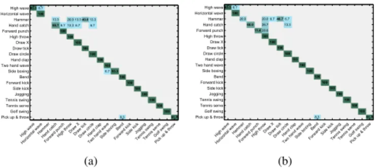
In order to show the accuracy of the approach on individual actions, the confusion matrix is also computed. Figure 5 shows the confusion matrix when we use the kNN and the Karcher mean per action and per subject with the full skeleton (Fig. 5a) and with body parts (Fig. 5b).
High wav e Horiz onta l wav e Ham mer Hand catch Forw ard pu nch High th row Draw X Draw tick Draw circle Hand clap Two hand wav e Side b oxingBend Forw ard kick Side ki ck Jogg ing Tenn is sw ing Tenn is serv e Golf s wing Pick u p & thro w 93.3 6.7 100 13.3 20.0 13.3 40.0 13.3 66.7 6.7 13.3 6.7 6.7 100 100 100 100 100 100 100 6.7 93.3 100 100 100 100 100 100 100 8.3 91.7 High wave Horizontal wave Hammer Hand catch Forward punch High throw Draw X Draw tick Draw circle Hand clap Two hand wave Side boxing Bend Forward kick Side kick Jogging Tennis swing Tennis serve Golf swing Pick up & throw
0 0.1 0.2 0.3 0.4 0.5 0.6 0.7 0.8 0.9 1 (a) High wav e Horiz onta l wav e Ham mer Hand catch Forw ard pu nch High thro w Draw X Draw tick Draw circle Hand clap Two hand wav e Side b oxingBend Forw ard kick Side ki ck Jogg ing Tenn is sw ing Tenn is serv e Golf s wing Pick u p & thro w 93.3 6.7 100 20.0 20.0 6.7 46.7 6.7 60.0 26.7 13.3 71.4 28.6 100 100 100 100 100 100 100 100 100 100 100 100 100 100 8.3 91.7 High wave Horizontal wave Hammer Hand catch Forward punch High throw Draw X Draw tick Draw circle Hand clap Two hand wave Side boxing Bend Forward kick Side kick Jogging Tennis swing Tennis serve Golf swing Pick up & throw
0 0.1 0.2 0.3 0.4 0.5 0.6 0.7 0.8 0.9 1 (b)
Fig. 5: MSR Action 3D. Confusion matrix for two variations of our approach: (a) Full skeleton with kNN and Karcher mean per action and per subject; (b) Body parts with kNN and Karcher mean per action and per subject.
It can be noted that for each variation of our approach, we obtained very low accuracies for the actions hammer and hand catch. This can be explained by the fact that these actions are very similar to some others. In addition, the way of performing these two actions varies a lot depending on the subject. For example, for the action hammer, subjects in the training set perform it only once, while some subjects in the test set perform it more than once (cyclically). In this case, the shape of the trajectories is very different. Our method does not deal with this kind of variations. Figure 6 illustrates an example of this failure case. As action sequences are represented in high dimension space, trajectories corresponding to only one joint (the right hand joint) are plotted. Indeed, the trajectories of four different samples of the action hammer are illustrated, where only one hammer stroke or two hammer strokes are performed. It can be observed that the shape of the trajectories is different in the two cases. In order to visualize samples of three different classes in a two-dimensional space, the Multidimensional scaling (MDS) technique [40] is applied using distance matrix computed on the shape space. These classes are shown in the right part of the figure: horizontal arm
wave (clear blue), hammer (dark blue) and draw tick (green). We can see that samples of the action hammer are split in two different clusters corresponding to two different ways of performing the action. The distribution of data in the hammer cluster is partly overlapped to data in the draw tick cluster yielding inaccurate classification of these samples.
(a) (b) (c) (d)
(b) (c) (d)
(a)
Fig. 6: Visualization of a failure case for the action hammer. Sample trajectories of the right hand joint are shown on the left: (a-b) one hammer stroke; (c-d) two hammer strokes. On the right, clustering of action samples using MDS in a 2D space is reported for three different classes: horizontal arm wave (clear blue), hammer (dark blue) and draw tick (green). The samples of the action hammer are split in two clusters corresponding to the two different ways of performing the action. The distribution of data of the hammer cluster is partly overlapped to data of the draw tick cluster
.
2) Florence 3D Action dataset: Results obtained for this dataset are reported in Table III. It can be observed that the proposed approach outperforms the results obtained in [39] us-ing the same protocol (leave-one-subject-out cross validation), even if we do not use the body parts variant.
TABLE III: Florence 3D Action. We compare our method with the one presented in [39].
Method Accuracy (%)
NBNN + parts + time [39] 82.0
Our Full Skeleton 85.85
Our Body part 87.04
By analyzing the confusion matrix of our method using body parts separately (see Fig. 7a), we can notice that the proposed approach obtains very high accuracies for most of the actions. However, we can also observe that there is some confusion between similar actions using the same group of joints. This can be observed in the case of read watch and clap hands, and also in the case of arm wave, drink and answer phone. For these two groups of actions, the trajectories of the arms are very similar. For the first group of actions, in most of the cases, read watch is performed using the two arms, which is very similar to the action clap hands. For the second group of actions, the main difference between the three actions is the object held by the subject (no object, a bottle, a mobile phone). As we use only skeleton features, we cannot detect and differentiate these objects. As an example, Figure 8 shows two different actions, drink and phone call, that in term of skeleton
are similar and difficult to distinguish.
Arm wave Drin k Phon e call Clap han ds Lace Sit dow n Stan d up Watch Bend 95.0 5.0 15.0 80.0 5.0 5.0 18.3 61.7 15.0 96.0 4.0 100 100 100 15.0 23.3 61.7 100 Arm wave Drink Phone call Clap hands Lace Sit down Stand up Watch Bend 0 0.1 0.2 0.3 0.4 0.5 0.6 0.7 0.8 0.9 1 (a) Walk Si t Stand Pick up Carry Thro w Push Pull Wave Clap 95.0 5.0 100 100 100 15.0 5.0 80.0 5.0 70.0 25.0 5.0 5.0 90.0 100 100 20.0 80.0 Walk Sit Stand Pickup Carry Throw Push Pull Wave Clap (b)
Fig. 7: Confusion matrix obtained by our approach on (a) Florence 3D Action and (b) UTKinect. We can see that similar actions involving different objects are confused.
(a) (b)
Fig. 8: Example of similar actions from Florence action 3D dataset: (a) drink action where the subject holds a bottle; (b) phone call action, where the subject holds a phone.
3) UTKinect dataset: In order to compare to the work in [9], we follow the same experimental protocol (leave one sequence out cross validation method). For each iteration, one sequence is used as test and all the other sequences are used as training. The operation is repeated such that each sequence is used once as testing. We obtained an accuracy of 91.5%, which improves the accuracy of 90.9% reported in [9]. This shows that our method is robust to different points of view and also to occlusions of some parts of the body. However, by analyzing the confusion matrix in Fig. 7b, we can notice that lower accuracies are obtained for those actions that include the interaction with some object, for instance the carry and throw actions. These actions are not always distinguished by actions that are similar in terms of dynamics yet not including the interaction with some object, like walk and push, respectively. This result is due to the fact that our approach does not take into account any informative description of objects.
4) Discussion: Results on different datasets show that our approach outperforms most of the state-of-the-art methods. First, some skeleton based methods like [10] use skeleton features based on pairwise distances between joints. However, results obtained on MSR Action 3D dataset show that ana-lyzing how the whole skeleton evolves during the sequence is more discriminative than taking into consideration the joints separately. In addition, the method proposed in [10] is not invariant to the execution speed. To deal with the execution speed, in [39] a pose-based method is proposed. However, the lack of information about temporal dynamics of the action makes the recognition less effective compared to our method, as shown in Table III. Second, the comparison with depth-map based methods shows that skeleton joints extracted from
depth-maps are effective descriptors to model the motion of the human body along the time. However, results also show that using strength of both depth and skeleton data may be a good solution as proposed in [20]. The combination of both data can be very helpful especially for the case of human-object interaction, where skeleton based methods are not sufficient as shown by the experiments on UTKinect dataset.
C. Representation and Invariance
1) Body Parts Analysis: The experiments above show that using only the moving parts of the body yields an improve-ment of the recognition accuracy. In addition, it allows the reduction of the dimensionality of the trajectories and thus the computational costs for their comparison. As we do not use the spine of the skeleton, the dimensionality is reduced at least to 48D instead of 60D. Furthermore, for the actions that are performed with only one part of the body, the dimensionality is reduced to only 12D (in the case of skeletons with four joints per limb).
2) Invariance to geometric transformations: To demon-strate the effectiveness of our invariant representation against translation and rotation, we analyze the distance between sequences representing the same action class, but acquired from different viewpoints. To this end, we select two samples from the UTKinect dataset corresponding to the action wave, and compute the distance between them with and without our invariant representation. We can see in Table IV that the distance drops from 1.1 to 0.6 if we use our invariant representation. We also compute the distance between actions belonging to similar classes, like wave and clap. It can be noticed that if we do not use the invariant representation, the nearest sample to the test sample belongs to the class clap; however, if the invariant representation is used, the nearest sample belongs to the class wave, the same as the test sample. TABLE IV: Distances between a wave sample and two sam-ples of the actions wave and clap acquired from different viewpoints. The columns ‘aligned’ and ‘non-aligned’ report the distance value computed with the invariant representation or without it, respectively.
wave sample clap sample
non-aligned aligned non-aligned aligned
wave sample 1.1 0.6 1.0 0.9
3) Rate Invariant: One main challenge in action recog-nition is robustness to variations in the execution speed of the action. Without this invariance, two instances of the same action performed at different velocities can be miss-classified. That is why temporal matching between two trajectories is decisive before computing their distance. The Dynamic Time Warping algorithm is usually employed to solve this problem. It is a popular tool in temporal data analysis, which is used in several applications, including activity recognition by video comparison [28]. In our case, a special version of this algo-rithm is used to warp similar poses of two sequences at differ-ent time instants. Before computing the distance between two
trajectories, we search for the optimal re-parametrization of the second trajectory with respect to the first one. This registration allows us to compare the shape of two trajectories regardless of the execution speed of the action. In practice, we use Dynamic Programming to find the optimal re-parametrization and perform registration. To show the importance of this step, we performed the same experiments presented above for two datasets, but without considering the registration step before comparison. The obtained results are presented in Table V. TABLE V: Results of the proposed method in the case the registration step is considered (R) or not (NR).
Method MSR Act. 3D (%) Florence Act. 3D (%)
kNN Full Skeleton - NR 73.9 82.1
kNN Full Skeleton - R 88.3 85.9
kNN Body parts - NR 73.5 84.7
kNN Body parts - R 91.1 87.0
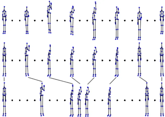
We can notice that skipping the registration step makes the accuracy much lower, especially for the MSR Action 3D dataset, where the accuracy drops of about 20%. In this dataset, actions are performed at very different speed. Figure 9 shows an example of the action high throw performed by two different subjects at different speed: The first row represents eight frames of a training sequence; The second row represents the same eight frames of a new sequence performed at different speed without registration; The third row represents the new sequence after registration with respect to the training sequence. In the reported case, the distance between sequences decreases from 1.31 (without registration) to 0.95 (with registration).
Fig. 9: Temporal registration for action high throw. From the top: the initial sequence; the sequence to be registered with respect to the initial sequence; the resulting registered sequence. Black lines connect corresponding poses showing how the sequence has been stretched and bent.
D. Latency Analysis
The latency is defined as the time lapse between the instant when a subject starts an action and the instant when the system recognizes the performed action. The latency can be separated into two main components: the computational latency and the
observational latency. The computational latency is the time the system takes to compute the recognition task from an observation. The observational latency represents the amount of time an action sequence needs to be observed in order to gather enough information for its recognition.
1) Computational Latency: We evaluate the computational latency of our approach on the MSR Action 3D dataset. Using a Matlab implementation with an Intel Core i-5 2.6GHz CPU and a 8GB RAM, the average time required to compare two sequences is 50 msec (including trajectories representation in shape space, trajectories registration, distance computation between trajectories, and sequence labeling using kNN). For a given new sequence, the total computational time depends on the number of training sequences. Indeed, distances between the new sequence and all other training sequences have to be computed, and the k shortest distances are used to label the new sequence. For example, using the 50-50 cross subject protocol on the MSR Action 3D dataset, and using only the kNN approach, classification of an unknown sequence requires comparison to 266 training sequences. Thus, with our approach, the system takes 266 ⇤ 0.05 = 13.3 sec to label a new sequence. This computational time is large and thus not suitable for real-time processing. If we use the Karcher mean per class to have only one representative sequence per class, the number of training sequences is reduced to 20 and the computational time decreases to 1 sec, which is more adequate for real-time applications. As shown in Table I, for this dataset we obtain our best accuracy using Karcher mean per action per subject. In that case, the resulted number of training trajectories is 91. Thus, the computational latency becomes 91 ⇤ 0.05 = 4.55 sec.
TABLE VI: Average computational time to compare two sequences of the MSR Action 3D dataset (the average length of sequences in this dataset is 38 frames). It results that more than 60% of the time is spent in the registration step.
Step representationshape-space registration distance labelingkNN Total
Time (s) 0.011 0.032 0.002 0.005 0.05
2) Observational Latency: To analyze the observational latency of our approach, we show how the accuracy depends on the duration of observation of the action sequence. In the first experiment, the observational latency is analyzed on the MSR Action 3D dataset, where the accuracy is computed by processing only a fraction of the sequence. In each case, we cut the training sequences into shorter ones to create a new training set. During the classification step, we also cut test sequences to the corresponding length and apply our method. We performed experiments using only kNN and also using Karcher mean per action and per subject. In Fig. 10a, we can see that an accuracy closed to the maximum one is obtained even if we use only half of the sequences. This shows that the computational latency can be masked by the observational latency in the cases where sequences are longer than twice the computational latency. In these cases, the action recognition task can be performed in real-time. This is particularly convenient for applications like video games
that require fast response of the system before the end of the performed action to support real-time interaction.
10 20 30 40 50 60 70 80 90 100 0 20 40 60 80 100 Frames (%) A cc ur ac y (%)
KNN & Karcher mean Only KNN (a) 5 10 15 20 25 30 35 40 45 50 55 60 0 10 20 30 40 50 60 70 80 90 100 Maximum Frames A cc ur ac y (%) LAL CRF BoW Our (b)
Fig. 10: Latency Analysis. (a) MSR Action 3D: Our approach is performed using only the kNN (blue curve), and then using the Karcher mean (red curve). (b) UCF-Kinect. Values of the accuracy obtained by our approach using only the kNN, compared to those reported in [11]. The accuracy at each point of the curves is obtained by processing only the number of frames shown in the x-axis.
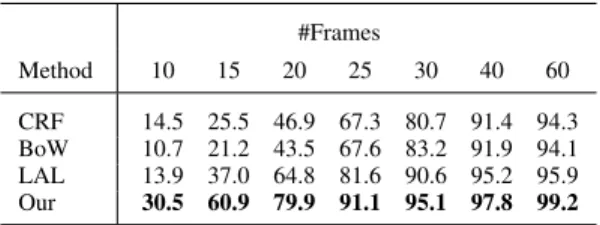
To compare the observational latency of our approach, we perform experiments on the UCF-Kinect dataset [11], where the observational latency of other methods is also evaluated. The same experimental setup as in Ellis et al. [11] is followed. To do that, we use only the kNN and a 4-fold cross validation protocol. Four subjects are selected for test and the others for training. This is repeated until each subject is used once. Actually, since there are 16 subjects, four different test folds are built and the mean accuracy of the four folds is reported. For a fair comparison to [11], the obtained accuracy is reported with respect to the maximum number of frames (and not to a percentage of sequences). For each step, a new dataset is built cutting the sequences to a maximum number of frames. The length of the sequences varies from 27 to 269 frames with an average length equal to 66.1 ±34 frames. It should be noticed that, if the number of frames of a sequence is below the maximum number of frames used in experiments, the whole sequence is treated. We compare our results with those reported in [11], including their proposed approach Latency Aware Learning (LAL), and two baseline solutions: Bag of Words (BoW) and Conditional Random Field (CRF). The observational latency on this dataset is also evaluated in [20], but following a different evalaution protocol (i.e., a 70/30 split protocol instead of the 4-fold cross validation proposed in [11]), so their results are not reported here.
The curves in Fig. 10b and the corresponding numerical re-sults in Table VII show that our approach clearly outperforms all the baseline approaches reported in [11]. This significant improvement is achieved either using a small or a large number of frames (see the red curve in Fig. 10b).
We can also notice that only 25 frames are sufficient to guarantee an accuracy over 90%, while BoW and CRF show a recognition rate below 68%, and LAL achieves 81.65%. It is also interesting to notice that using the whole sequences, we obtain an accuracy of 99.15%, and the same accuracy can be obtained by processing just 45 frames of the sequence.
TABLE VII: Numerical results at several points along the curves in Fig. 10b. #Frames Method 10 15 20 25 30 40 60 CRF 14.5 25.5 46.9 67.3 80.7 91.4 94.3 BoW 10.7 21.2 43.5 67.6 83.2 91.9 94.1 LAL 13.9 37.0 64.8 81.6 90.6 95.2 95.9 Our 30.5 60.9 79.9 91.1 95.1 97.8 99.2
VI. CONCLUSIONS ANDFUTUREWORK
An effective human action recognition approach is proposed using a spatio-temporal modeling of motion trajectories in a Riemannian manifold. The 3D position of each joint of the skeleton in each frame of the sequence is represented as a motion trajectory in the action space. Each motion trajectory is then expressed as a point in the open curve shape space. Thanks to the Riemannian geometry of this manifold, action classification is solved using the nearest neighbor rule, by warping all the training points to the new query trajectory and computing an elastic metric between the shape of trajectories. The experimental results on the MSR Action 3D, Florence 3D Action and UTKinect datasets demonstrate that our approach outperforms the existing state-of-the-art methods in most of the cases. Furthermore, the evaluation in terms of latency clearly demonstrates the efficiency of our approach for a rapid recognition. In fact, 90% action recognition accuracy is achieved by processing just 25 frames of the sequence. Thereby, our approach can be used for applications of human action recognition in interactive systems, where a robust real-time recognition at low latencies is required.
As future work, we plan to integrate in our framework other descriptors based on both depth and skeleton information, so as to manage the problem of human-object interaction. We also expect widespread applicability in domains such as physical therapy and rehabilitation.
ACKNOWLEDGMENTS
A very preliminary version of this work appeared in [41]. The authors would like to thank Professor Anuj Srivastava for his assistance and the useful discussions about this work.
REFERENCES
[1] Microsoft Kinect, 2013. [Online]. Available:
http://www.microsoft.com/en-us/kinectforwindows/
[2] ASUS Xtion PRO LIVE, 2013. [Online]. Available:
http://www.asus.com/Multimedia/Xtion PRO/
[3] J. Shotton, A. Fitzgibbon, M. Cook, T. Sharp, M. Finocchio, R. Moore, A. Kipman, and A. Blake, “Real-time human pose recognition in parts from single depth images,” in Proc. IEEE Int. Conf. on Computer Vision and Pattern Recognition, Colorado Springs, Colorado, USA, June 2011, pp. 1–8.
[4] S. Hadfield and R. Bowden, “Kinecting the dots: Particle based scene flow from depth sensors,” in Proc. Int. Conf. on Computer Vision, Barcelona, Spain, Nov. 2011, pp. 2290–2295.
[5] Z. Ren, J. Yuan, and Z. Zhang, “Robust hand gesture recognition based on finger-earth mover’s distance with a commodity depth camera,” in Proc. ACM Int. Conf. on Multimedia, Scottsdale, Arizona, USA, Nov. 2011, pp. 1093–1096.
[6] S. Berretti, A. Del Bimbo, and P. Pala, “Superfaces: A super-resolution model for 3D faces,” in Proc. Work. on Non-Rigid Shape Analysis and Deformable Image Alignment, Florence, Italy, Oct. 2012, pp. 73–82. [7] J. Han, L. Shao, D. Xu, and J. Shotton, “Enhanced computer vision
with microsoft kinect sensor: A review.” IEEE Trans. on Cybernetics, vol. 43, no. 5, pp. 1318–1334, 2013.
[8] L. Liu and L. Shao, “Learning discriminative representations from RGB-D video data,” in Proc. of the Twenty-Third Int. Joint Conf. on Artificial Intelligence, ser. IJCAI’13. AAAI Press, 2013, pp. 1493–1500. [9] L. Xia, C.-C. Chen, and J. K. Aggarwal, “View invariant human action
recognition using histograms of 3D joints,” in Proc. Work. on Human Activity Understanding from 3D Data, Providence, Rhode Island, USA, June 2012, pp. 20–27.
[10] X. Yang and Y. Tian, “Eigenjoints-based action recognition using naive-bayes-nearest-neighbor,” in Proc. Work. on Human Activity Understand-ing from 3D Data, Providence, Rhode Island, June 2012, pp. 14–19. [11] C. Ellis, S. Z. Masood, M. F. Tappen, J. J. La Viola Jr., and R.
Suk-thankar, “Exploring the trade-off between accuracy and observational latency in action recognition,” Int. Journal on Computer Vision, vol. 101, no. 3, pp. 420–436, 2013.
[12] W. Li, Z. Zhang, and Z. Liu, “Action recognition based on a bag of 3D points,” in Proc. Work. on Human Communicative Behavior Analysis, San Francisco, California, USA, June 2010, pp. 9–14.
[13] X. Yang, C. Zhang, and Y. Tian, “Recognizing actions using depth motion maps-based histograms of oriented gradients,” in Proc. ACM Int. Conf. on Multimedia, Nara, Japan, Oct. 2012, pp. 1057–1060. [14] A. W. Vieira, E. R. Nascimento, G. L. Oliveira, Z. Liu, and M. F.
Campos, “STOP: Space-time occupancy patterns for 3D action recogni-tion from depth map sequences,” in Iberoamerican Congress on Pattern Recognition, Buenos Airies, Argentina, Sept. 2012, pp. 252–259. [15] J. Wang, Z. Liu, J. Chorowski, Z. Chen, and Y. Wu, “Robust 3D action
recognition with random occupancy patterns,” in Proc. Europ. Conf. on Computer Vision, Florence, Italy, Oct. 2012, pp. 1–8.
[16] L. Xia and J. K. Aggarwal, “Spatio-temporal depth cuboid similarity feature for activity recognition using depth camera,” in Proc. CVPR Work. on Human Activity Understanding from 3D Data, Portland, Oregon, USA, June 2013, pp. 2834–2841.
[17] O. Oreifej and Z. Liu, “HON4D: Histogram of oriented 4D normals for activity recognition from depth sequences,” in Proc. Int. Conf. on Computer Vision and Pattern Recognition, Portland, Oregon, USA, June 2013, pp. 716–723.
[18] B. Ni, Y. Pei, P. Moulin, and S. Yan, “Multi-level depth and image fusion for human activity detection,” IEEE Trans. on Cybernetics, vol. 43, no. 5, pp. 1383–1394, Oct 2013.
[19] J. Wang, Z. Liu, Y. Wu, and J. Yuan, “Mining actionlet ensemble for action recognition with depth cameras,” in Proc. IEEE Conf. on Computer Vision and Pattern Recognition, Providence, Rhode Island, USA, June 2012, pp. 1–8.
[20] E. Ohn-Bar and M. M. Trivedi, “Joint angles similarities and HOG2
for action recognition,” in Proc. CVPR Work. on Human Activity Understanding from 3D Data, Portland, Oregon, USA, June 2013, pp. 465–470.
[21] D. Weinland, R. Ronfard, and E. Boyer, “A survey of vision-based meth-ods for action representation, segmentation and recognition,” Computer Vision and Image Understanding, vol. 115, no. 2, pp. 224–241, Feb. 2011.
[22] P. Turaga, R. Chellappa, V. S. Subrahmanian, and O. Udrea, “Machine recognition of human activities: A survey,” IEEE Trans. on Circuits and Systems for Video Technology, vol. 18, no. 11, pp. 1473–1488, Nov. 2008.
[23] W. Bian, D. Tao, and Y. Rui, “Cross-domain human action recognition,” IEEE Trans. on Systems, Man, and Cybernetics, Part B: Cybernetics, vol. 42, no. 2, pp. 298–307, Apr. 2012.
[24] R. Poppe, “A survey on vision-based human action recognition,” Image Vision Comput., vol. 28, no. 6, pp. 976–990, Jun. 2010.
[25] L. Liu, L. Shao, X. Zhen, and X. Li, “Learning discriminative key poses for action recognition,” IEEE Trans. on Cybernetics, vol. 43, no. 6, pp. 1860–1870, Dec 2013.
[26] Y. Tian, L. Cao, Z. Liu, and Z. Zhang, “Hierarchical filtered motion for action recognition in crowded videos,” IEEE Transactions on Systems, Man, and Cybernetics, Part C: Applications and Reviews, vol. 42, no. 3, pp. 313–323, May 2012.
[27] L. Shao, X. Zhen, D. Tao, and X. Li, “Spatio-temporal laplacian pyramid coding for action recognition,” IEEE Trans. on Cybernetics, vol. 44, no. 6, pp. 817–827, 2014.


![TABLE III: Florence 3D Action. We compare our method with the one presented in [39].](https://thumb-eu.123doks.com/thumbv2/123doknet/12429588.334430/10.918.97.449.207.374/table-iii-florence-d-action-compare-method-presented.webp)